Digital Signal Processing

(1)

Prof. Dr. V. Stahl

Heilbronn University of Applied Sciences

November 29, 2021

(2)

1 Foundations

1.1 Dirac Impulse

Consider a rectangular function in the time window 0 ≤t < εand amplitude 1/ε:

dε(t) = ₁

ε if 0≤t < ε 0 else

The area under this function is independent ofεalways 1, i.e.

Z ∞

−∞

dε(t)dt = 1.

The function gets interesting whenεis very small. In that case the time duration approaches zero, the amplitude infinity. The result is the Dirac impulse or Delta functionδ:

δ(t) = lim_ε→0

ε>0

dε(t).

Actually the limit is not a real function in R→ R. Therefore δ(t) is called a generalized function or distribution. The essential properties ofδ(t) are

δ(t) = 0 ift6= 0

∞ ift= 0 and

Z ∞

−∞

δ(t)dt = 1.

We can do calculus with infinitely large numbers∞just as we do with infinitely small numbersdx. In both cases we merely use a simplified notation for a limit operation.

A rather useful property of the Dirac impulse is that it is an even function, i.e.

δ(t) = δ(−t).

As any other function we can shift the Dirac impulse to an arbitrary position t=aby

δ(t−a) =

0 ift6=a

∞ ift=a As the Dirac impulse is an even function, it holds that

δ(t−a) = δ(a−t).

If we multiply a functionf(t) with a shifted Dirac impulseδ(t−a) we obtain f(t)δ(t−a) = f(a)δ(t−a)

(4)

for allt wheref(t) is continuous. We can convince ourselves easily that this is correct: For t6=aboth sides are zero and for t=a we havef(a)δ(0) on both sides. From this we can deduce the sifting property of the Dirac impulse.

Theorem 1.1 (Sifting Property) Letf ∈R→R. Then it holds that

Z ∞

−∞

f(τ)δ(t−τ)dτ = f(t) for allt wheref(t)is continuous.

The proof is as follows:

Z ∞

−∞

f(τ)δ(t−τ)dτ = Z ∞

−∞

f(t)δ(t−τ)dτ

= f(t)Z ∞

−∞

δ(t−τ)dτ

= f(t).

(5)

1.2 Convolution

The convolutionf∗g of two functionsf, g is defined by (f ∗g)(t) = Z ∞

−∞

f(τ)g(t−τ)dτ.

Convolution is a binary function of functions like e.g. composition or addition of functions. Note that (f ∗g)(t) is definined only if the convolution integral converges. This is always presumed in the following.

Convolution is commutative, i.e.

f∗g = g∗f.

This is obtained from

(f∗g)(t) = Z ∞ τ=−∞

f(τ)g(t−τ)dτ with the substitutionµ=t−τ unddτ =−dµ:

Z ∞ τ=−∞

f(τ)g(t−τ)dτ = Z −∞

µ=∞

−f(t−µ)g(µ)dµ

= Z ∞ µ=−∞

g(µ)f(t−µ)dµ

= Z ∞ τ=−∞

g(τ)f(t−τ)dτ

= (g∗f)(t).

What happens if we convolve a function f with a Dirac impulse δ? From Theorem 1.1 it follows that

(f ∗δ)(t) = Z ∞

−∞

f(τ)δ(t−τ)dτ

= f(t) and hence

f∗δ = f.

The Dirac impulse is therefore the neutral element of convolution.

When we attach an index ˆtat a function we mean from now on that the function is shifted by ˆt, i.e.

fˆt(t) = f(t−ˆt) for all t.

Convolving a function f with a shifted Dirac impulse has the effect that the

(6)

function is shifted:

(f∗δtˆ)(t) = Z ∞

−∞

f(τ)δˆt(t−τ)dτ

= Z ∞

−∞

f(τ)δ(t−ˆt−τ)dτ

= Z ∞

−∞

f(t−ˆt)δ(t−ˆt−τ)dτ

= f(t−tˆ)Z ∞

−∞

δ(t−tˆ−τ)dτ

= f(t−tˆ). Therefore it holds that

f ∗δ_ˆ_t = f_ˆ_t.

Convolution has many other properties, some of which are summarized in the following theorem.

Theorem 1.2 (Convolution)

f∗δ = f f ∗δˆt = fˆt

f∗g = g∗f (f∗g)∗h = f∗(g∗h)

a(f∗g) = (af)∗g

(f1+f2)∗g = (f1∗g) + (f2∗g) fˆt∗g = (f∗g)ˆt.

Convolution has a neutral elementδ. Convolution with a shifted Dirac impulse causes shifting. Convolution is commutative and associative. The next two properties express that convolution is a linear operation. The last property is called time invariance. The proofs are not difficult and almost trivial if we use the convolution theorem of Fourier Transform.

(7)

1.3 Fourier Series

Theorem 1.3

Letf(t)be a piece wise continuousT-periodic signal. Then there exist A_k andϕ_k such that

f(t) = A₀+

∞

X

k=1

A_kcos(kωt+ϕ_k), ω=2π T for allt wheref(t)is continuous.

A T-periodic signal can be presented as an overlay of harmonic oscillations whose frequencies are entire multiples of the fundamental frequencyω= 2π/T. We can simplify this sum somewhat with complex numbers.

f(t) = A0+

∞

X

k=1

Akcos(kωt+ϕk)

= A₀+

∞

X

k=1

re

Ake^j(kωt+ϕ^k⁾

= A₀+

∞

X

k=1

re A_ke^jϕ^ke^jkωt

= A₀+1 2

∞

X

k=1

A_ke^jϕ^ke^jkωt+A_ke^jϕ^ke^jkωt

= A0+1 2

∞

X

k=1

Ake^jϕ^ke^jkωt+Ake^−jϕ^ke^−jkωt

= A0+

∞

X

k=1

1

2Ake^jϕ^ke^jkωt+

∞

X

k=1

1

2Ake^−jϕ^ke^−jkωt

= A0

|{z}

z0

+

∞

X

k=1

1 2Ake^jϕ^k

| {z }

zk, k=1,2,...

e^jkωt+

−∞

X

k=−1

1

2A−ke^−jϕ^−k

| {z }

zk, k=−1,−2,...

e^jkωt

= z0+

∞

X

k=1

zke^jkωt+

−1

X

k=−∞

zke^jkωt

=

∞

X

k=−∞

z_ke^jkωt where

z0 = A0

z_k = ₁

/2A_ke^jϕ^k f"urk >0

1/2A_−ke^−jϕ^−k f"urk <0.

(8)

For example

z₃ = 1 2A₃e^jϕ³ z₋₃ = 1

2A3e^−jϕ³

= z3.

The Fourier coefficientsz_k appear in conjugate complex pairs, i.e.

z_−k = z_k.

From Fourier coefficient z_k we can obtain amplitude and phase of the k-th harmonic:

A0 = z0

A_k = 2|zk|

ϕk = ^(zk), k= 1,2, . . .

In order to compute the n-th Fourier coefficient z_n of function f(t) we begin with the equation

f(t) =

∞

X

k=−∞

zke^jkωt and multiply both sides withe^−jnωt:

f(t)e^−jnωtdt =

∞

X

k=−∞

zke^jkωte^−jnωtdt.

Integration fromt= 0, . . . , T on both sides gives Z T

0

f(t)e^−jnωtdt = Z T 0

∞

X

k=−∞

zke^jkωte^−jnωtdt

=

∞

X

k=−∞

zk

Z T 0

e^j(k−n)ωtdt.

The integral can be solved as follows:

• If k=nwe have Z T

0

e^j(k−n)ωtdt = Z T 0

1dt = T.

(9)

• If k6=nwe have Z T

0

e^j(k−n)ωtdt = 1 j(k−n)ω

he^j(k−n)ωti^T

0

= 1

j(k−n)ω

e^j(k−n)ωT −1

ω= 2π/T

= 1

j(k−n)ω

e^2πj(k−n)−1

k−n∈Z

= 1

j(k−n)ω(1−1)

= 0 Hence

Z T 0

e^j(k−n)ωtdt =

T ifk=n 0 else.

and therefore Z T

0

f(t)e^−jnωtdt =

∞

X

k=−∞

z_k Z T

0

e^j(k−n)ωtdt

| {z } T ifk=n, 0 else

= znT or

zn = 1 T

Z T 0

f(t)e^−jnωtdt.

Theorem 1.4 (Fourier Series)

Letf ∈R→Rbe aT-periodic funcion and zk = 1

T Z T

0

f(t)e^−jkωtdt whereω= 2π/T. Then it holds that

f(t) =

∞

X

k=−∞

zke^jkωt

for allt wheref(t)is continuous.

(10)

1.4 Fourier Transform

The decomposition into a Fourier series is only defined forT-periodic functions f(t). In order to analyze also non-periodic functions in the frequency domain we take the limitT → ∞. A periodic function whose period duration is infinitely long is actually a non-periodic function. This is the basic idea behind the transition from Fourier series to Fourier Transform.

Definition 1.5 (Fourier Transform) The function

F(ω) = Z ∞

−∞

f(t)e^−jωtdt is called Fourier Transform off(t). Inversely

f(t) = 1 2π

Z ∞

−∞

F(ω)e^jωtdω is called inverse Fourier Transform ofF(ω).

The most important properties of the Fourier Transform are summarized in the appendix.

Analogy between Fourier Series and Fourier Transform.

• In the Fourier Series of a T-periodic function f(t) the Fourier coefficient zktells us the amplitude and phase of thek-th harmonic in the frequency decomposition off(t).

• In analogy

1

2πF(ω)dω

tells us the amplitude and phase of the oscillation with frequency ω in the frequency decomposition of f(t). Because of factor dω every single oscillation has only infinitesimal amplitude provided thatF(ω) is finite.

In analogy to the physical mass density function we call F(ω) therefor spectral density function: Every point has only infinitesimal mass. In order to obtain the mass of an object we have to integrate his density function.

(11)

2 Sampling and Aliasing

2.1 Fourier Series of the Pulse Train

Let

p(t) =

∞

X

n=−∞

δ(t−nT).

Visuallyp(t) is an of an infinte sequence of Dirac pulses with distanceT. There- forep(t) is also called pulse train Dirac comb.

−T

−2T

−3T T 2T 3T

p(t)

t

· · ·

As the pulse train isT-periodic, we can decompose it into a Fourier series p(t) =

∞

X

k=−∞

zke^jkωt, ω=2π T .

In order to avoid that during the computation of Fourier coefficient zk pulses appear at the integration limits we do not integrate from 0 to T but rather from −^T/2to^T/2. If a periodic function is integrated over an entire period it is irrelevant where to start.

zk = 1 T

Z T 0

p(t)e^−jkωtdt

= 1

T Z T /2

−T /2

p(t)e^−jkωtdt

= 1

T Z T /2

−T /2

δ(t)e^−jkωtdt

= 1

T Z T /2

−T /2

δ(t)e⁰dt

= 1

T Z T /2

−T /2

δ(t)dt

= 1

T.

The Fourier coefficients zk of the pulse train are all equal ¹/T. Therefore the Fourier series of the pulse train is

p(t) = 1 T

∞

X

k=−∞

e^jkωt.

(12)

2.2 Sampling

Time continuous signalsf(t) can be processed by a digital computer only after sampling. This means that we consider only function values off(t) at discrete points in time nT_s whereT_sis the sampling interval. The sampled values are

fn = f(nTs), n∈Z.

Sampling is often carried out by multiplication with a puse train p(t) =

∞

X

n=−∞

δ(t−nTs). The result is

fp(t) = f(t)p(t)

= f(t)

∞

X

n=−∞

δ(t−nT_s)

=

∞

X

n=−∞

f(t)δ(t−nTs)

=

∞

X

n=−∞

f(nTs)δ(t−nTs)

=

∞

X

n=−∞

f_nδ(t−nT_s)

The sampled signalfp(t) consits of a sequence of pulses with distanceTswhere the pulse at time nTs is multiplied by samplefn.

t

· · · fp(t)

· · ·

f₋2

f₋1

f1

f2

f3

f₋3

f0

3Ts

2Ts

Ts

−T s

−2Ts

−3Ts

Probably you wonder why sampling is done in such a complicated way: The sampled signalfp(t) is an intermediate step between analogue and discrete. On the one hand sidefp(t) is still a time continuous function oft, on the other side fp(t) depends only on the samplesfn. This way we can apply all theory from analog functions and especially Fourier Transform tofp(t) and thereby transfer it to discrete signals. Further, f(t) and fp(t) are actually not as different as it seems at a first glance. For smallTsthe area underf(t) andfp(t) is almost the

(13)

same:

Z ∞

−∞

f_p(t)dt = Z ∞

−∞

∞

X

n=−∞

f_nδ(t−nT_s)

=

∞

X

n=−∞

fn

Z ∞

−∞

δ(t−nTs)

=

∞

X

n=−∞

fn

= 1

T_s

∞

X

n=−∞

fnTs

≈ 1 T_s

Z ∞

−∞

f(t)dt.

This does not only hold for the entire area from−∞to∞but also for the area over finite intervals.

(14)

2.3 Aliasing

What is the effect of sampling f(t) in the frequency domain? If we use the Fourier series of the pulse train as derived in Section 2.1, we obtain

fp(t) = f(t)p(t)

= f(t) 1 T_s

∞

X

k=−∞

e^jkω^s^t

= 1

Ts

∞

X

k=−∞

f(t)e^jkω^s^t.

The Fourier Transform Fp(ω) of fp(t) is obtained from the Fourier Transform F(ω) off(t) and the correspondence

f(t)e^j^ωt^ˆ c s F(ω−ωˆ). With ˆω=kωswe have

f(t)e^jkω^s^t c s F(ω−kωs). From linearity of Fourier Transform it follows that

1 Ts

∞

X

k=−∞

f(t)e^jkω^s^t

| {z } fp(t)

c s 1 Ts

∞

X

k=−∞

F(ω−kωs)

| {z } Fp(ω)

.

This result can be interpreted as follows: F(ω−kω_s) is the Fourier Transform F(ω) of the original functionf(t) shifted bykωs. The sum

∞

X

k=−∞

F(ω−kωs)

consists of infinitely many copies of F(ω) shifted by ω_s on the frequency axis.

Hence

F_p(ω) = 1 T_s

∞

X

k=−∞

F(ω−kω_s)

consists of infinitely many copies ofF(ω) shifted byωsand scaled by¹/Ts. If the copies overlap, the overlapping parts are summed up. In that case F(ω) can no longer be obtained fromFp(ω) by cutting out one copy and scale it with Ts. This phenomenon is called Aliasing. The higher the sampling frequencyωs

is, i.e. the more samples per second we take, the farther lie the copies of F(ω) apart and the less likely overlapping occurs.

Let’s keep in mind:

Sampling withTs c s Periodic continuation withωs

and scaling with¹/T_s.

(15)

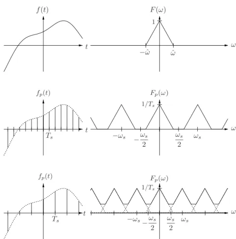
f(t)

t

Ts t

Ts

t ω

ω

ω 1

−ωˆ ωˆ

ωs

2

−ωs

2

Fp(ω)

−ωs ωs ωs

−ωs 2 2 f_p(t)

fp(t)

1/Ts

Fp(ω) F(ω)

Figure 2.1: Top: Band limited signal f(t) with cutoff frequency ˆω and Fourier Transform F(ω). Middle: Sampled signal f_p(t) =f(t)p(t). The sampling rate ω_s = 2π/T_s ist larger than 2ˆω, therefore no aliasing. The copies of F(ω) do not overlap. Bottom: Sampling rate ωs ist smaller than 2ˆω, therefore aliasing occurs. The copies ofF(ω) overlap.

(16)

2.4 Band-Limited Signals

A functionf ∈R→Ris called band-limited with cutoff frequency ˆω if F(ω) = 0 for allω with|ω| ≥ω.ˆ

Informally this means that f(t) has no oscillation components with frequency above or equal ˆω.

Aliasing, i.e. an overlap in the frequency domain after sampling is avoided if the copies of F(ω) have distance more than 2ˆω on the frequency axis. The conditions to avoid aliasing are therefore:

• The signal f(t) has to be band-limited with cutoff frequency ˆω.

• The sampling rateωshas to be sufficiently high, i.e.

ωs>2ˆω.

(17)

3 Signal Reconstruction with Low Pass Filter- ing

After the samples of a signal have been processed in a digital computer an analog signal has to be reconstructed from the resulting, discrete samples. This step is called digital-analog conversion.

With a small modification of the theory presented in this chapter we can also build frequency selective digital filters. Filtering is done in a digital computer by discrete convolution.

3.1 Signal Reconstruction

As shown above, the Fourier Transform offp(t) consists of infinitely many copies ofF(ω) shifted byωs. We assume in the following that the signalf(t) was band- limited with cutoff frequency ˆωand the sampling frequencyω_swas high enough, i.e.

ω_s/>2ˆω.

This means that the assumptions of the sampling theorem are satisfied and the copies ofF(ω) inF_p(ω) do not overlap.

For signal reconstruction we merely have to cut out one of these copies, scale it with Ts and transform it with the inverse Fourier Transform back into time domain.

Cutting out a copy in the frequency range

−ωs

2 < ω < ωs

2

and scaling withTsis accomplished by multiplication with a rectangular func- tionG(ω) in the frequency domain

G(ω) =

Ts if|ω|< ωs/2 0 else.

Multiplying Fp(ω) and G(ω) in the frequency domain gives the Fourier Trans- form F(ω) of the original time signalf(t):

F(ω) = Fp(ω)G(ω)

= 1

T_s

∞

X

k=−∞

F(ω−kωs)

| {z }

Fp(ω)

G(ω).

The signalf(t) usually comes from a sensor and is not given by a closed math- ematical term. ThereforeF(ω) cannot be computed analytically and the multiplication withG(ω) has to be done by convolution in time domain. Acoording to the convolution theorem we have

(fp∗g)(t) c s F(ω)G(ω).

(18)

The inverse Fourier Transform g(t) ofG(ω) is obtained as follows:

g(t) = 1 2π

Z ∞

−∞

G(ω)e^jωtdω

= T_s 2π

Z ω_s/2

−ωs/2

e^jωtdω

= Ts

2πjt

e^jωt^ωs/2

−ωs/2

= T_s πt

1 2j

e^jω^s^t/2+e^−jω^s^t/2

= Ts

πt im

e^jω^s^t/2

= T_s

πt sin(ωst/2)

= T_s πtsin

πt Ts

daω_s=2π Ts

= siπt Ts

= sinc(t/Ts). where

si(x) = sin(x)/x fallsx6= 0 1 fallsx= 0 sinc(x) = si(πx).

From the samples

f_k = f(kT_s)

we can reconstruct now the continuous signalf(t) for everyt∈Ras follows by convolution in time domain.

f(t) = (f_p∗g)(t)

=

∞

X

k=−∞

fkδ(t−kTs)

!

| {z }

fp(t)

∗g(t)

=

∞

X

k=−∞

fk(g(t)∗δ(t−kTs)) (Linearity of convolution)

=

∞

X

k=−∞

fkg(t−kTs) (Convolution with shifted impulse)

=

∞

X

k=−∞

f_k sinc

t−kT_s Ts

=

∞

X

k=−∞

fk sinc (t/Ts−k).

(19)

Theorem 3.1 (Sampling Theorem)

Letf(t)be band-limited with cutoff frequencyωˆ and fk =f(kTs), k=−∞, . . . ,∞, Ts=2π

ω_s. Let the sampling rateω_s be big enough, i.e.

ωs>2ˆω.

Thenf(t)can be reconstructed exactly from the samplesfk by f(t) =

∞

X

k=−∞

fksinc (t/Ts−k).

(20)

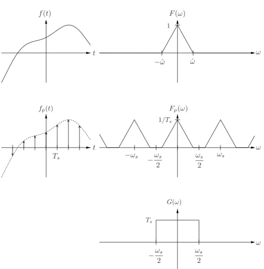
t

f(t)

fp(t)

ω

ω F(ω)

ˆ

−ωˆ ω

t

−ωs

2

ωs

−ωs ωs

2 Fp(ω)

G(ω)

ωs

−ωs 2 2 Ts

1/Ts

1

Ts

Figure 3.1: Top: Band-limited signalf(t) with cutoff frequency ˆω and Fourier Transform F(ω). Middle: Sampled signal fp(t) =f(t)p(t). The sampling rate ωs= 2π/Tsis higher than 2ˆω, hence the copies ofF(ω) do not overlap. Bottom:

Rectangular function G(ω), which is multiplied with Fp(ω) to obtain F(ω) in frequency domain.

(21)

3.2 Low Pass Filter

With the results of the previous section we will show now how to do realize a low pass filter with a given cutoff frequencyω_c. Filteringf(t) means that its Fourier Transform F(ω) has to be set to zero for allω with|ω| ≥ω_c. As according to the Sampling Theoremf(t) is already band-limited with cutoff frequencyω_s/2, low pass filtering makes only sense for

ωc< ωs

2 .

In order to implement this operation in time domain on samples we merely have to adapt the rectangular functionG(ω), which was used in the previous section for signal reconstruction by replacing the cut out range

h−ωs

2 ,ωs

2 i with

[−ωc, ωc].

We obtain a new rectangular function for low pass filtering G(ω) =

Ts if|ω|< ωc

0 else.

The product

H(ω) = F_p(ω)G(ω)

is now the Fourier Transform of the low pass filtered signal h(t).

As in the previous section multiplication in frequency domain has to be done with convolution in time domain. As before we obtaing(t) with inverse Fourier Transform:

g(t) = 1 2π

Z ∞

−∞

G(ω)e^jωtdω

= Ts

2π Z ω_c

−ωc

e^jωtdω

= Ts

2πjt e^jω^c^t−e^−jω^c^t

= T_s

πtsin(ωct)

= 2

ωstsin(ω_ct)

= 2ωc

ω_s 1

ω_ctsin(ω_ct)

= 2ωc

ω_s si(ω_ct)

The low pass filtered signal h(t) is obtained by convolution h(t) = (fp∗g)(t).

(22)

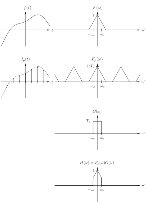
ωc

−ωc

ωc

−ωc

ωc

−ωc

ωc

−ωc

f(t)

ω ω

ω

ω F(ω)

fp(t)

t

G(ω) Fp(ω)

H(ω) =Fp(ω)G(ω) 1/Ts

Ts

1 1

Figure 3.2: From top to bottom: Band limited signalf(t) and F(ω). Sampled signalfp(t) andFp(ω). Transfer functionG(ω) of the low pass filter with cutoff frequencyωc. Low pass filtered signalH(ω).

(23)

A low pass filter is a linear time invariant system with impulse response g(t).

For the practical computation there are two problems:

• The impulse response has infinite length which makes a practical computation impossible.

• The system is non-causal, i.e. g(t)6= 0 fort <0. Low pass filtering can therefore not be done in real time without delays.

Both problems are solved as follows:

• Asg(t) is a si-function, its function values are small for absolutely larget and can be set to zero fort >ˆtfor some suitable ˆt. This is done in time domain by multiplication with a rectangular functionr(t) where

r(t) =

0 if|t| ≥ˆt 1 else.

By replacing the impulse response g(t) with g(t)r(t) we have a system withfiniteimpulse resonse.

Instead of cutting the impulse response “hard” at±ˆt with a rectangular functionr(t) we can also use a soft window function. A common choice is the Hamming Window:

˜

r(t) = 0 if|t| ≥ˆt 0.54 + 0.46 cos(πt/ˆt) else.

1

−ˆt ˆt

t

˜ r(t)

• The impulse responseg(t)r(t) is now limited to the range−ˆt,ˆt

but still not causal. This can be rectified if we shift it by ˆt. As shifting one factor in a convolution has the effect that the result of the convolution is shifted by the same amount we get merely a shift in the low pass filtered signal h(t) by ˆt. A short time delay is often acceptable in practical applications.

Summarizing, instead of the original impulse response g(t) we work with the modified causal and finite impulse response

x(t) = g(t−ˆt)r(t−ˆt) withx(t) = 0 fort6∈0,2ˆt.

(24)

The choice of ˆt requires a compromise: A big value of ˆt causes small errors as only small function values ofg(t) are set to zero. On the other hand a big value of ˆt causes large delays and high computation costs as shown below.

The (approximately) low passed filtered and by ˆtdelayed signalh(t) is obtained in the same way as for signal reconstruction in the previous section.

h(t) = (f_p∗x)(t)

=

∞

X

k=−∞

fkδ(t−kTs)

!

∗x(t)

=

∞

X

k=−∞

f_k(δ(t−kT_s)∗x(t))

=

∞

X

k=−∞

fkx(t−kTs).

From this continuous signalh(t) we now take samplesh_`. h_` = h(`T_s)

=

∞

X

k=−∞

fkx(`Ts−kTs)

=

∞

X

k=−∞

fkx((`−k)Ts)

=

∞

X

k=−∞

f_kx_`−k

= (f∗x)`.

The convolution in the last line is calleddiscreteconvolution of the samplesf_k andxk of the signalsf(t) and the impulse responsex(t).

Definition 3.2 (Discrete Convolution)

The discrete convolution of two sequencesf` andg`is defined as (f∗g)` =

∞

X

k=−∞

fkg_`−k.

In order to obtain a simple representation of the filter coefficients x_k, let ˆ

t = n

2Ts

for some integern. From

x(t) = g(t−ˆt)r(t−ˆt)

= 2ωc

ω_s si(ω_ct−tˆ)r(t−ˆt)

(25)

we obtain

xk = x(kTs)

= 2ω_c

ωs si(ω_c(kT_s−ˆt))r(kT_s−tˆ)

= 2ω_c

ωs si(ω_c(k−n/2)T_s)r((k−n/2)T_s)

= 2ω_c ωs si

2πω_c

ωs (k−n/2)

r_k−n/2

= 2ω_c ωs sinc

2ω_c

ωs (k−n/2)

r_k−n/2

= ˆωcsinc(ˆωc(k−n/2))r_k−n/2 where

ˆ

ωc = 2ω_c ωs

is the normalized cutoff frequency with−1<ωˆc <1.

As the impuse response x(t) has finite length due to windowing, only finitely many filter coefficients x_k are non-zero. Which ones is determined as follows:

For the window function it holds that

r(t) = 0 for|t| ≥ˆt . Replacingt by (k−n/2)Ts on both sides we obtain

r((k−n/2)T_s) = 0 for

k−n 2

T_s ≥ n

2T_s and hence

r_k−n/2= 0 for k−n

2 ≥n

2 or

r_k−n/2= 0 fork≥noderk <0.

Therefore only filter coefficientsxk are non-zero fork= 0, . . . , n−1.

For the rectangular window we have

r_k−n/2 = 1, k= 0, . . . , n−1

and the multiplication with 1 can be ignored during the computation of the

(26)

filter coefficients. For the Hamming Window we have

˜

r_k−n/2 = r((k−n/2)Ts)

= 0.54 + 0.46 cosπ(k−n/2)Ts

ˆ t

= 0.54 + 0.46 cosπ(k−n/2)Ts

nTs/2

= 0.54 + 0.46 cos

π(2k−n) n

= 0.54 + 0.46 cos 2πk

n −π

= 0.54−0.46 cos 2πk

n

, k= 0, . . . , n−1.

Summary. The filter coefficients of the low pass filter with cutoff frequency ωc of lengthnare given by

xk = ˆωcsinc(ˆωc(k−n/2)), k= 0, . . . , n−1 where ˆω_c is the normalized cutoff frequency

ˆ

ω_c = 2ωc

ω_s .

The low pass filter causes an additional delay of the signal by ˆ

t = n

2Ts

or n/2 cycles.

As the impulse response was cut out to obtain finite length we merely obtain an approximation which is more accurate the more coefficientsnthe filter uses.

In addition we can improve the result by using a Hamming Window. Doing so we have to multiplyxk with

wk = 0.54−0.46 cos 2πk

n

, k= 0, . . . , n−1.

The samplesh` of the low pass filtered signal are computed by discrete convolution

h` =

∞

X

k=−∞

fkx_`−k

=

∞

X

k=−∞

f_`−kx_k

=

n−1

X

k=0

f_`−kxk.

(27)

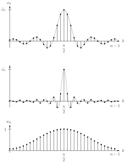
xk

ˆ ωc

wk

1 ˆ ωc

k

k n−1

n−1

n−1 n

2 n 2

n 2

Figure 3.3: Coefficients of the low pass filter xk of length n= 32 for ˆωc = 0.3 (top) und ˆωc = 0.8 (middle). The lower figure shows the weights wk of the Hamming window.

(28)

3.3 Windowing

^∗

Probably you wondered in the last section why Hamming Windowing should be an improvement over a simple rectangular window and why of all things the Hamming Window is chosen and not some other window function.

The purpose of windowing was to truncate the infinite impulse responseg(t) to a finite interval [−ˆt,ˆt]. This is accomplished by multiplication with a window functionr(t). What is the effect iff(t) is not convolved with the ideal, infinite impulse responseg(t) but with a truncated versiong(t)r(t)?

Let us compare g(t) and g(t)r(t) in the frequency domain. While G(ω) is an ideal rectangle and hence cuts out the desired frequency range precisely, we have to compute the Fourier Transform of g(t)r(t) by convolution in the frequency domain:

g(t)r(t) c s 1

2π(G∗R)(ω).

If R(ω) = 2πδ(ω) were an impulse, windowing with r(t) would not cause any distortion. However, in this case we would haver(t) = 1 and thus would not be limited to [−ˆt,ˆt]. A “good” windowing functionr(t) should therefore have the property that its Fourier Transform R(ω) is as close as possible to 2πδ(ω).

For the rectangular window r(t) =

0 if|t| ≥tˆ 1 else the Fourier Transform is

R(ω) = 2ˆtsi(ωˆt).

The constant factor 2ˆt causes merely scaling. The shape of the curve is determined by the factor si(ωˆt), which does not look like an impulse. For large values ofωˆtthe function value is very small. Hence, if ˆtis large, the magnitude of R(ω) is significant only near ω = 0. Near ω = 0 the value ofR(ω) is very large due to the multiplication with 2ˆt. Thus for large ˆt it is in fact true that R(ω) converges to an impulse. This was expected as for a large window width ˆt only very small values ofg(t) are truncated.

Let us consider now the Hamming Window

˜ r(t) =

0 falls|t| ≥tˆ

a+bcos(πt/ˆt) sonst witha= 0.54 andb= 0.46. Its Fourier Transform is

R˜(ω) = a2ˆtsi(ωˆt)

| {z }

R(ω)

+bˆt si(ωˆt−π) + si(ωˆt+π) .

We obtain a weighted sum ofR(ω) and two by ±π shifted si-functions. These additional summands are chosen such that the disturbing side lobes in R(ω)

(29)

cancel out and a much smoother curve results, see picture 3.4. Hence the ideal transfer functionG(ω) is much less distorted by a Hamming Window than it is by a rectangular window.

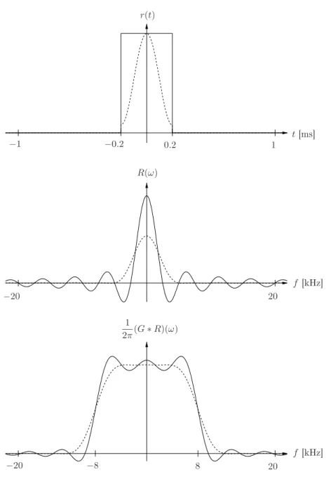
The figure below shows a comparison between the rectangular window (solid line) and the Hamming Window (dashed line). A signal is filtered with cutoff frequency ω_c = 2π×8kHz. The impulse response of the filter is truncated at ˆ

t= 0.2ms. Depicted is the audible frequency range up to 20kHz.

(30)

1

2π(G∗R)(ω) R(ω)

r(t)

−0.2 0.2 1

−1

t^[ms℄

−20 20

−8

−20 20

f^[kHz℄

8

Figure 3.4: Top: Window functions r(t) in time domain. Middle: Fourier TransformsR(ω) of the window functions. Bottom: The distorted transfer functions by windowing, which would ideally be a rectangle. Rectangular window:

solid line, Hamming Window: dashed line.

(31)

1

2π(G∗R)(ω) R(ω)

r(t)

−1 1

t^[ms℄

−20 20

−8

−20 20

f^[kHz℄

−0.6 0.6

8

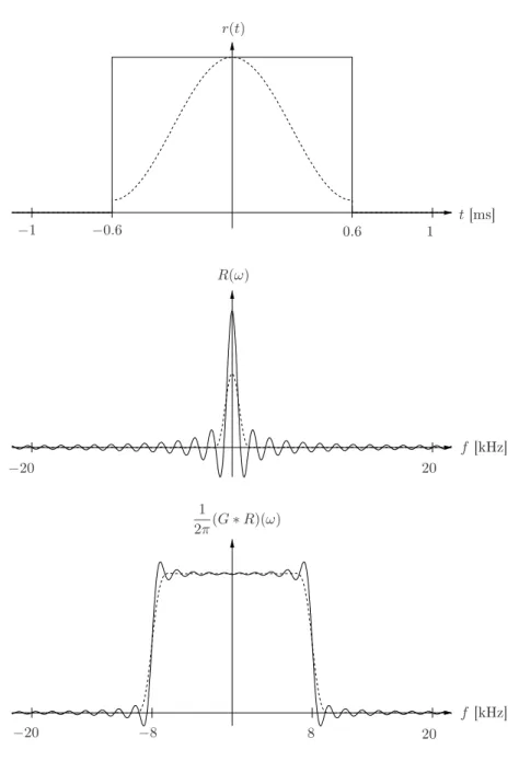
Figure 3.5: Same figure as above, except that the window width has been increased from 0.2ms to 0.6ms. G(ω) is now closer to an impulse and the transfer function is much less distorted.

(32)

3.4 Discrete Time Fourier Transform

^∗

There is a second way to compute the Fourier TransformF_p(ω) off_p(t).

Starting with

fp(t) =

∞

X

n=−∞

fnδ(t−nTs) we obtain from the correspondence

δ(t−nTs) c s e^−jnωT^s the Fourier Transform

fp(t) c s X^∞

n=−∞

fne^−jnωT^s

| {z } Fp(ω)

.

We can computeFp(ω) either directly from the samples fn or fromF(ω):

Fp(ω) =

∞

X

k=−∞

F(ω−kωs)

=

∞

X

n=−∞

f_ne^−jnωT^s

From both presentations we see immediately thatFp(ω) is periodic with period ωs, i.e.

Fp(ω+ωs) = Fp(ω) for allω.

By rescaling the frequency axis we can normalize the sampling interval to 1.

ForT_s= 1 it holds that

Fp(ω) =

∞

X

n=−∞

fne^−jnω.

This transformation of a sequence fn is called discrete time Fourier Transform (DTFT). Hence Fp(ω) ist nothing but the z-Transform of fn for z =e^jω, i.e.

forz on the unit circle.

FromF_p(ω) we obtain by inverse Fourier Transform the original pulse train fp(t) and thus the samples fn. However, there is also a direct way: First, we multiply both sides withe^jkω

Fp(ω)e^jkω =

∞

X

n=−∞

fne^−jnωe^jkω and then integrate forω from 0 to 2π:

Z 2π 0

Fp(ω)e^jkωdω = Z 2π 0

∞

X

n=−∞

fne^−jnωe^jkωdω

=

∞

X

n=−∞

fn

Z 2π 0

e^j(k−n)ωdω

(33)

As

Z 2π 0

e^j(k−n)ωdω = 2π ifk=n 0 else it follows that

Z 2π 0

Fp(ω)e^jkωdω = 2πfk

or

f_k = 1 2π

Z 2π 0

F_p(ω)e^jkωdω.

The difference to the invese Fourier Transform of F_p(ω) which would have re- sulted in the impulse trainf_p(t) is, that we integrate only from 0 to 2πand not from −∞bis∞.

Summarizing, the DTFT and its inverse are defined as follows. The correspondence is also valid if the assumptions of the Sampling Theorem are violated.

We can obtain fromFp(ω) always the samplesfkexactly but notf(t) if the sampling rate was too low.

Definition 3.3 (Discrete Time Fourier Transform)

The Discrete Time Fourier Transform (DTFT) of the sequence fk is defined by

Fp(ω) =

∞

X

k=−∞

fke^−jkω.

Its inverse is

fk = 1 2π

Z 2π 0

Fp(ω)e^jkω.

(34)

4 Discrete Fourier Transform

4.1 Band-limited Periodic Signals

Letf(t) be aT0-periodic signal with Fourier series f(t) =

∞

X

k=−∞

z_ke^jkω⁰^t, ω₀= 2π/T₀.

Further, assumef(t) is band-limited with cutoff frequency ˆω. This means that only finitely many Fourier Coefficientsz_kare non-zero, which is shown as follows:

With the correspondence

e^jkω⁰^t c s 2πδ(ω−kω0) we obtain the Fourier Transform F(ω) off(t):

F(ω) = 2π

∞

X

k=−∞

z_kδ(ω−kω₀). Asf(t) is band-limited,F(ω) = 0 forω≥ωˆ and hence

zk= 0 if kω0≥ωˆ i.e. if k≥ ωˆ ω0

.

The signal is sampled during one period atnequidistant places. The sampling rate is therefore

ωs = nω0.

The conditions of the Sampling Theorem hold, i.e. we assume ω_s>2ˆω.

It follows that

n 2 > ωˆ

ω0

and therefore

zk = 0 if k≥ n 2.

In the Fourier series only finitely many summands remain and it holds that

f(t) =

n/2−1

X

k=−n/2+1

zke^jkω⁰^t

=

n/2−1

X

k=−n/2+1

zke^jkω^s^t/n.

(35)

For the samples f_`=f(`T_s) we have

f` =

n/2−1

X

k=−n/2+1

zke^jk`ω^s^T^s^/n

=

n/2−1

X

k=−n/2+1

zke^2πjk`/n.

Cosmetics. For rewriting this formula in vector notation, the sum f_` =

n/2−1

X

k=−n/2+1

z_ke^2πjk`/n has to be transformed into a sum

f` =

n−1

X

k=0

. . . .

For this puropse we define Fourier Coefficientsz_k fork=n/2, . . . , n−1, which do not appear in the original sum and which were zero so far as

z_n/2 = 0

z_k = z_k−n, k=n/2 + 1, . . . , n−1,

see figure 4.1. This way we can rewrite the summands with negativek.

−1

X

k=−n/2+1

zke^2πjk`/n =

n−1

X

k=n/2+1

zk−ne2πj(k−n)`/n

=

n−1

X

k=n/2+1

z_ke^2πjk`/ne^−2πjn`/n

=

n−1

X

k=n/2+1

zke^2πjk`/ne^−2πj`

| {z }

=1

=

n−1

X

k=n/2+1

z_ke^2πjk`/n.

(36)

For the entire sum it holds that

f` =

n/2−1

X

k=−n/2+1

zke^2πjk`/n

=

−1

X

k=−n/2+1

zke^2πjk`/n+

n/2−1

X

k=0

zke^2πjk`/n

=

n−1

X

k=n/2+1

zke^2πjk`/n+

n/2−1

X

k=0

zke^2πjk`/n

=

n−1

X

k=0

z_ke^2πjk`/n.

2

1 3

−1

−2

−3

5 6 7

z1

z2

z3

z1

z2

z3

z1

z2

z3

z1

z2

z3

k k

2

1 3 4

Figure 4.1: Example for n = 8. The coefficients z_k with k = −1,−2,−3 are shifted tok= 7,6,5.

Digital Signal Processing

Prof. Dr. V. Stahl

Heilbronn University of Applied Sciences

November 29, 2021

Contents

1 Foundations

1.1 Dirac Impulse

1.2 Convolution

1.3 Fourier Series

1.4 Fourier Transform

2 Sampling and Aliasing

2.1 Fourier Series of the Pulse Train

2.2 Sampling

2.3 Aliasing

2.4 Band-Limited Signals

3 Signal Reconstruction with Low Pass Filter- ing

3.1 Signal Reconstruction

3.2 Low Pass Filter

3.3 Windowing

3.4 Discrete Time Fourier Transform

4 Discrete Fourier Transform

4.1 Band-limited Periodic Signals