Seasonal Cycles in European Agricultural Commodity Prices

IHS Economics Series Working Paper 192

September 2006

Seasonal Cycles in European Agricultural Commodity Prices

Adusei Jumah

Robert M. Kunst

Impressum Author(s):

Adusei Jumah, Robert M. Kunst Title:

Seasonal Cycles in European Agricultural Commodity Prices ISSN: Unspecified

2006 Institut für Höhere Studien - Institute for Advanced Studies (IHS) Josefstädter Straße 39, A-1080 Wien

E-Mail: o ce@ihs.ac.atffi Web: ww w .ihs.ac. a t

All IHS Working Papers are available online: http://irihs. ihs. ac.at/view/ihs_series/

This paper is available for download without charge at:

https://irihs.ihs.ac.at/id/eprint/1726/

Seasonal Cycles in European Agricultural Commodity Prices

Adusei Jumah, Robert M. Kunst

192

Reihe Ökonomie

Economics Series

192 Reihe Ökonomie Economics Series

Seasonal Cycles in European Agricultural Commodity Prices

Adusei Jumah, Robert M. Kunst September 2006

Institut für Höhere Studien (IHS), Wien

Institute for Advanced Studies, Vienna

Contact:

Adusei Jumah

Department of Economics and Finance Institute for Advanced Studies

Stumpergasse 56 1060 Vienna, Austria and

Department of Economics University of Vienna Brünner Straße 72 1210 Vienna, Austria

email: adusei.jumah@univie.ac.at Robert M. Kunst

Department of Economics and Finance Institute for Advanced Studies Stumpergasse 56

1060 Vienna, Austria and

University of Vienna Department of Economics Brünner Straße 72 1210 Vienna, Austria

email: robert.kunst@univie.ac.at

Founded in 1963 by two prominent Austrians living in exile – the sociologist Paul F. Lazarsfeld and the economist Oskar Morgenstern – with the financial support from the Ford Foundation, the Austrian Federal Ministry of Education and the City of Vienna, the Institute for Advanced Studies (IHS) is the first institution for postgraduate education and research in economics and the social sciences in Austria.

The Economics Series presents research done at the Department of Economics and Finance and aims to share “work in progress” in a timely way before formal publication. As usual, authors bear full responsibility for the content of their contributions.

Das Institut für Höhere Studien (IHS) wurde im Jahr 1963 von zwei prominenten Exilösterreichern – dem Soziologen Paul F. Lazarsfeld und dem Ökonomen Oskar Morgenstern – mit Hilfe der Ford- Stiftung, des Österreichischen Bundesministeriums für Unterricht und der Stadt Wien gegründet und ist somit die erste nachuniversitäre Lehr- und Forschungsstätte für die Sozial- und Wirtschafts- wissenschaften in Österreich. Die Reihe Ökonomie bietet Einblick in die Forschungsarbeit der Abteilung für Ökonomie und Finanzwirtschaft und verfolgt das Ziel, abteilungsinterne Diskussionsbeiträge einer breiteren fachinternen Öffentlichkeit zugänglich zu machen. Die inhaltliche Verantwortung für die veröffentlichten Beiträge liegt bei den Autoren und Autorinnen.

Abstract

This paper explores the seasonal cycles of European agricultural commodity prices. We focus on three food crops (barley, soft and durum wheat) and on beef. We investigate whether seasonality is deterministic or unit-root stochastic and whether seasonal cycle for specific agricultural commodities have converged over time. Finally, we develop time-series models that are capable of forecasting agricul-tural prices on a quarterly basis.

Firstly, we find that seasonal cycles in agricultural commodity prices are mainly deterministic and that evidence on common cycles across countries varies over agricultural commodities.

The prediction experiments, however, yield a ranking with respect to accuracy that does not always match the statistical in-sample evidence.

Keywords

Seasonal cycles, seasonal unit roots, forecasting, agricultural commodities

JEL Classification

C32, C53, Q11

Comments

We wish to thank Jose Luis Gallego for helpful comments on an earlier version. The usual proviso applies.

Contents

1 Introduction 1

2 Data description 3

2.1 Barley ... 3

2.2 Wheat ... 5

2.3 Beef ... 6

3 Univariate HEGY tests 8 4 Multivariate evidence 13 5 Forecasting 18

5.2 Forecasting the barley price series ... 20

5.3 Forecasting the wheat price series ... 21

5.4 Forecasting the beef price series ... 23

6 Summary and conclusion 23

References 25

1 Introduction

This paper explores the seasonal cycles of European agricultural commod- ity prices. We investigate whether seasonality is deterministic or unit-root stochastic and whether seasonal cycles for speci…c agricultural commodities have converged over time. Finally, we develop time-series models that are capable of forecasting agricultural prices on a quarterly basis.

In order to identify the seasonal cycles in agricultural commodity prices, the test strategy of Hylleberg et al. (1990, HEGY) is applied to panels of quarterly prices of four di¤erent agricultural commodities: barley, soft and durum wheat, and beef. The main …nding is that seasonal cycles are deterministic and repetitive. This indicates that the direct in‡uence of the climatic cycle dominates any possible technological developments in farming.

Our results correspond to those reported by Palaskas and Crowe (1996) who …nd that the seasonality of soft wheat prices is mainly determin- istic. We …nd similar results for much longer data series, additional countries, and additional commodities. The general impression persists when we ap- ply the test due to Canova and Hansen (1995), which uses deterministic seasonality as its null and seasonal unit roots as its alternative. However, there are occasional contrary test results. We conjecture that the seasonal cycle may indeed be subject to slow changes in some countries but that these changes are too small to admit modelling by low-order autoregressions with seasonal unit roots, which would be appropriate for forecasting.

Given that seasonality is deterministic, the next issue of concern is whether it coincides across countries. Harvesting seasons di¤er slightly across Europe but completely independent patterns are also unlikely, at least at the quar- terly frequency. Because of the adoption of similar technology by di¤erent countries and of increasing international integration, one may expect that seasonal patterns show some signs of convergence across Europe. To explore this hypothesis, we use a new monitoring technique that was suggested by Franses and Kunst (2005). We …nd that evidence on common seasonality varies somewhat among di¤erent commodities.

Apart from a possible coincidence at the seasonal frequency, one may also expect common movements of agricultural prices at the long-run frequency, i.e. cointegration. However, the empirical evidence on cointegration between countries remains weak. For the complete panels, cointegration is generally not supported on statistical grounds.

The issues of forecasting and of seasonality are closely related, as the seasonal cycle is typically the most predictable frequency band of a time series (see Sargent, 2001). We note, however, that in-sample selection of seasonal models does not necessarily correspond to the ranking in prediction

1

experiments (see Kunst, 1993).

In contrast to the traditional strategy in forecasting, which subjects fore- casting models to rigorous statistical tests and discards misspeci…ed models, we adopt an alternative technique. A set of potential prediction models is created, and these models are subjected to a horse race of out-of-sample predictions over the last part of the available data. The set includes mod- els that have been rejected on statistical grounds, such as the cointegrating model. We …nd that assumed cointegration indeed implies a deterioration in forecasting performance. In contrast, the— usually rejected— restriction of common seasonal cycles improves predictive accuracy in most cases. This result conforms to the basic pattern that simpler and restricted models often are bene…cial for forecasting, even when the restrictions fail to hold according to statistical in-sample tests.

Missing data turned out to be a major stumbling block for the direct appli- cation of time-series methods to the data panels. Interpolation of time-series data is a classical problem of econometric analysis (see, e.g., Friedman, 1962). We replace the missing data points by model-based forecasts, which in turn are then used in lieu of observations for the generation of predictions.

Using this strategy, we succeed in a partial elimination of the missing-values problem.

The remainder of the paper is structured as follows. Section 2 describes the data and presents some descriptive regressions on seasonal dummy vari- ables. Section 3 focuses on univariate HEGY tests. Section 4 analyzes the potential presence of common seasonal cycles. Section 5 reports the pre- diction experiments and also describes the interpolation techniques in some detail. Section 6 concludes.

2

2 Data description

Data are constructed from the Eurostat data base. Out of the various agri- cultural commodity prices, we restrict attention to three main food crops (barley, soft and durum wheat), for which an adequate number of observa- tions is available, and to beef. The beef price mainly serves as a control variable, as we conjecture that it shows less seasonal variation than the food crop prices. Monthly series were transformed to quarterly, which eased the identi…cation of seasonal cycles, as econometric methodology is better de- veloped and more precise at the quarterly frequency. This step also serves to eliminate some missing values. We note that, apart from the revealed missing values, monthly data remain constant for several successive months, which may point to hidden missing values in data sources. Furthermore, all data were transformed by logarithms, in line with the usual focus on rates of in‡ation that are well approximated— and often even de…ned— as di¤erences of logarithms.

While the original, monthly series contained many missing values, we succeeded in eliminating most of them by aggregating months to quarters.

As a general rule, we de…ned a quarterly price as the average of all observed monthly prices within that quarter. For example, if January is available but February and March are unobserved, the …rst quarter price is de…ned as the January price.

2.1 Barley

Barley is the most robust European food crop. It is grown in all EU countries.

However, the requirement of continuous price series of reasonable length re- stricts our analysis to twelve countries: Austria, Belgium, Germany, Den- mark, Spain, Finland, France, Italy, Netherlands, Portugal, Sweden, and the United Kingdom. The last column in Table 1 gives the time range of avail- able data for each country. While the start of the range usually coincides with the begin of the country’s membership in the EU, the end date may re-

‡ect some delays in reporting data. Time ranges vary a lot and are generally quite unsatisfactory for an analysis of longer-run features. For example, it is di¢ cult to determine whether seasonal cycles have changed over a range of as few as seven years. Statistical tests will have very little power for such series.

At …rst, we run ‘naive’ regressions of variables on quarterly dummies and report the identi…ed seasonal patterns and the R

. This is a traditional exploratory technique that has been suggested by Miron (1996), among oth- ers. In all countries excepting Belgium, the seasonal cycle in the barley price

3

series is substantial. Table 1 reports the percentages of total variation that are explained by seasonal dummies in log(P

), where P denotes the origi- nal barley price data. We also give the coe¢ cient estimates for the seasonal constants. Obviously, ‘barley in‡ation’ tends to be highest in the …rst and fourth quarters, while it is slightly lower in the second and considerably lower in the third or summer quarter, when usually barley is harvested. One may conjecture that a drop in price increases in the second quarter is more typical for southern Europe, where the harvest season may start earlier. While there is some evidence in favor of this conjecture in Spain, Italy, and Portugal, we note that there is also a negative second-quarter coe¢ cient in Finland.

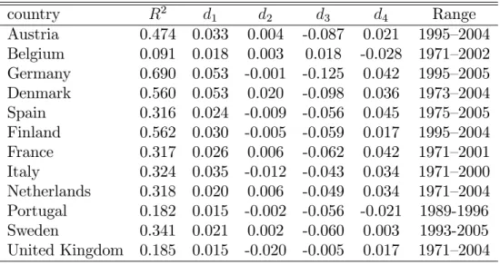
Table 1: Deterministic seasonality in the growth rate of barley prices.

country R

d

d

d

d

Range

Austria 0.474 0.033 0.004 -0.087 0.021 1995–2004 Belgium 0.091 0.018 0.003 0.018 -0.028 1971–2002 Germany 0.690 0.053 -0.001 -0.125 0.042 1995–2005 Denmark 0.560 0.053 0.020 -0.098 0.036 1973–2004 Spain 0.316 0.024 -0.009 -0.056 0.045 1975–2005 Finland 0.562 0.030 -0.005 -0.059 0.017 1995–2004 France 0.317 0.026 0.006 -0.062 0.042 1971–2001 Italy 0.324 0.035 -0.012 -0.043 0.034 1971–2000 Netherlands 0.318 0.020 0.006 -0.049 0.034 1971–2004 Portugal 0.182 0.015 -0.002 -0.056 -0.021 1989-1996 Sweden 0.341 0.021 0.002 -0.060 0.003 1993-2005 United Kingdom 0.185 0.015 -0.020 -0.005 0.017 1971–2004

Figure 1 depicts the typical seasonal cycle for barley prices, for conve- nience still on the basis of monthly data. We selected those countries where the most complete data are available: Belgium, Denmark, Spain, and the United Kingdom. The graph shows monthly means for the logarithms of the price levels. For Denmark, Spain, and the UK, the graph corresponds to our interpretation that the harvest season— July in Spain and the UK, August in Denmark— causes a dip in prices. The Belgian prices attain a seasonal trough in October, following a peak in summer. From Table 1, it is obvious that Belgium is an exception. We conjecture that the non-intuitive seasonal pattern is caused by occasional irregularities and outliers.

4

Figure 1: Monthly seasonal cycle in logarithmic barley prices.

2.2 Wheat

Wheat comes mainly in two di¤erent species: common or bread wheat (Triticum aestivum) and hard or durum wheat (Triticum durum). There are also other species, whose cultivation is less widespread. Wheat is more demanding than barley, and its cultivation is therefore restricted to better soils and climates.

Particularly, the cultivation of durum wheat is concentrated in the Mediter- ranean.

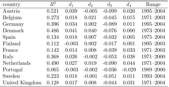
The strength and shape of the seasonal soft wheat cycle is comparable to the barley cycle. Price increases have a positive mean in the …rst and fourth quarter and a negative mean in the third quarter, again identi…ed with the most customary harvest season. The seasonal cycle is strongest in Austria and weakest in Finland. For all details, see Table 2.

For durum wheat, only four countries provide data of reasonable regular- ity, and even so one of the series is rather short: Austria, Spain, France, and Italy. While the explanatory power of the seasonal dummies remains mod- erate for these countries, Table 3 shows that the shape of the cycle remains fairly identical across them. The …rst and fourth quarter yield signi…cantly higher price increases than the second and third quarters. Typically, durum

5

Table 2: Deterministic seasonality in the growth rate of soft wheat prices.

country R

d

d

d

d

Range

Austria 0.521 0.039 -0.005 -0.099 0.026 1995–2004 Belgium 0.273 0.018 0.021 -0.045 0.015 1971–2003 Germany 0.396 0.034 0.002 -0.089 0.011 1995–2004 Denmark 0.486 0.041 0.040 -0.076 0.000 1973–2004 Spain 0.134 0.018 0.007 -0.032 0.005 1975–2004 Finland 0.112 -0.003 0.002 -0.017 0.001 1995–2003 France 0.142 0.014 0.008 -0.039 0.033 1971–2003 Italy 0.368 0.026 -0.002 -0.053 0.038 1971–2000 Netherlands 0.490 0.027 0.019 -0.090 0.044 1971–2004 Portugal 0.065 -0.003 -0.002 -0.036 -0.029 1989–2000 Sweden 0.223 0.018 -0.001 -0.051 0.011 1993–2004 United Kingdom 0.128 0.017 0.008 -0.044 0.031 1971–2004

prices fall in the second quarter and rise again in the last quarter of each year.

Table 3: Deterministic seasonality in the growth rate of durum wheat prices.

country R

d

d

d

d

Range

Austria 0.138 0.014 -0.011 -0.050 0.014 1995–2004 Spain 0.208 0.025 -0.036 -0.034 0.021 1985–2004 France 0.308 0.003 -0.011 -0.010 0.027 1971–2003 Italy 0.138 0.026 -0.018 -0.032 0.026 1971–2000

2.3 Beef

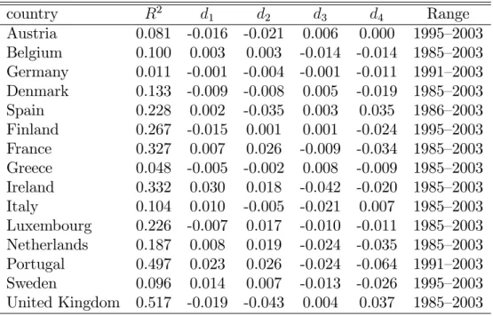
As stated earlier, we also investigated animal product prices. For the example of beef, Table 4 shows the identi…ed deterministic seasonal structure. Given that breeding and slaughtering take place throughout the year, seasonality turns out to be weak. R

remains low for some countries, and no common seasonal pattern across countries emerges from the table, even though sea- sonal constants are often signi…cant at a 5% level. For example, while many countries show a tendency toward falling prices at the end of the year, UK

6

prices rise in the fourth quarter, and the UK is the case with the strongest seasonality.

Table 4: Deterministic seasonality in the growth rate of beef prices.

country R

d

d

d

d

Range

Austria 0.081 -0.016 -0.021 0.006 0.000 1995–2003 Belgium 0.100 0.003 0.003 -0.014 -0.014 1985–2003 Germany 0.011 -0.001 -0.004 -0.001 -0.011 1991–2003 Denmark 0.133 -0.009 -0.008 0.005 -0.019 1985–2003 Spain 0.228 0.002 -0.035 0.003 0.035 1986–2003 Finland 0.267 -0.015 0.001 0.001 -0.024 1995–2003 France 0.327 0.007 0.026 -0.009 -0.034 1985–2003 Greece 0.048 -0.005 -0.002 0.008 -0.009 1985–2003 Ireland 0.332 0.030 0.018 -0.042 -0.020 1985–2003 Italy 0.104 0.010 -0.005 -0.021 0.007 1985–2003 Luxembourg 0.226 -0.007 0.017 -0.010 -0.011 1985–2003 Netherlands 0.187 0.008 0.019 -0.024 -0.035 1985–2003 Portugal 0.497 0.023 0.026 -0.024 -0.064 1991–2003 Sweden 0.096 0.014 0.007 -0.013 -0.026 1995–2003 United Kingdom 0.517 -0.019 -0.043 0.004 0.037 1985–2003

7

3 Univariate HEGY tests

According to Ghysels and Osborn (200), the most important time-series models for seasonality are deterministic, stationary stochastic seasonality, and seasonal unit roots models. Usually, stationary stochastic seasonality can be ignored, as it just describes some local and mean-reverting seasonal variation that needs no speci…c modeling. A main tool for discriminating de- terministic seasonality— which implies time-constant seasonal patterns— and seasonal unit roots— which describe persistently changing seasonal patterns—

is the test procedure due to Hylleberg et al. (1990), the so-called HEGY test.

Table 5 shows the results of applying the HEGY test procedure to the barley price series. In particular, the regression

4

X

= X

j=1

d

D

+ b

X

+ b

X

+ b

X

+ b

X

+ X

j=1

j 4

X

+ u

(1)

is estimated for X representing the logarithmic prices. Here,

denotes quarterly seasonal di¤erences X

X

,

denotes semi-annual di¤erences X

X

, while X

is the four-periods moving average X

+X

+X

+X

and X

is its counterpart with alternating signs X

X

+ X

X

. In the HEGY test, the t–statistics on the coe¢ cients b

and b

and the joint F –statistics on b

and b

are evaluated. These values t

, t

, and F

become signi…cant, when respective unit roots at 1, 1, and i are absent. In the literature, there are several suggestions on how to determine the lag order p+. We chose to minimize AIC for autoregressions of order p with added seasonal dummies and to set p+ = max(p 4; 0).

Table 5 shows that seasonal unit roots are rejected for most series. This indicates that the seasonal cycle has remained fairly constant over the whole time range. However, there is an annual seasonal unit root for Austria, and a semi-annual one for Portugal, which is however a fairly short series. In other words, there is evidence on persistent changes of the seasonal cycle for Austria and Portugal. In contrast, the unit root at 1 cannot be rejected for any country, which indicates that the levels of prices experience persistent changes and face no tendency of mean reversion.

As a means of control, we also give the statistics due to Canova and Hansen (1995, CH) that test for the null of stationarity of dummy-adjusted

…rst-order di¤erences X. While the results are in line with the HEGY

8

Table 5: HEGY tests for seasonal unit roots in the barley price series.

country p+ t

t

F

CH

Austria 0 -1.53 3.64** 0.36 0.60 Belgium 1 -2.06 3.09* 6.83* 1.94**

Germany 0 -1.48 4.82** 8.57* 0.67 Denmark 0 -2.10 7.03** 43.74** 1.90**

Spain 1 -1.34 6.69** 48.51** 0.47 Finland 0 -0.67 4.36** 6.26 y 0.81 France 0 -2.29 6.62** 32.39** 0.60 Italy 0 -2.65 6.47** 45.45** 0.91 y Netherlands 0 -2.07 7.16** 58.14** 1.01*

Portugal 0 -1.39 1.87 10.46** 0.42 Sweden 0 -0.75 5.46** 8.34* 0.54 United K. 2 -2.06 3.16* 18.57** 1.39**

Note: y denotes signi…cance at the 10% level, * at the 5% level, and ** at the 1% level. t

, t

, and F

are the HEGY test statistics for unit roots at +1, -1, and I. CH denotes the Canova-Hansen test statistic.

9

tests for most cases— noting that non-rejection for the CH tests corresponds to rejection for the HEGY tests— three countries reject their null hypotheses at the 1% level, and there are some additional borderline cases. The joint evaluation of HEGY and CH tests has been considered in the literature by Hylleberg (1995) and by Kunst and Reutter (2002), among others.

While both tests achieve some local optimization of power properties, the recommended decision on the basis of con‡icting results is not obvious. By means of Monte Carlo simulation with …xed parametric design, Hylleberg (1995) …nds that the decision based on the HEGY test is preferable for data- generating processes that conform to an autoregressive scheme. Kunst and Reutter (2002) …nd the stronger result that the HEGY test decision is usually preferable for a mixed simulation design with 50% autoregressions and 50% unobserved-components processes, where the latter species corre- sponds to the basic model for which the CH test was derived. Based on such results, one may conclude that Table 5 provides a summary evidence in favor of models without seasonal unit roots. Alternatively, and particularly in view of the fact that most con‡ict situations stem from longer series, one may take the results literally. According to the CH test, some price variables contain a signi…cant component with seasonal unit roots but an attempt to model these very same variable by an autoregression with seasonal unit roots fails according to the HEGY test. As our aim is developing prediction models on an autoregressive basis, we decided to discard the possibility of seasonal unit roots in our series for further analysis.

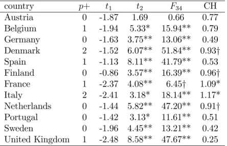
Table 6 shows the results of HEGY tests for the soft wheat price series.

Again, the tests reject the possible presence of seasonal unit roots in most variables convincingly. The only exception is the Austrian series, which this time provides evidence on persistent changes at both seasonal component frequencies. It is unfortunate that this country’s series is comparatively short, starting only from 1995, and it may also be infested by some data errors, as we suspect from some sudden price jumps. On the whole, the evidence on seasonal unit roots is scarce, and the seasonal variation in wheat prices and their changes is dominated by repetitive deterministic cycles.

The smaller data set for durum wheat agrees well with the other …eld crops. Table 7 shows that there is no evidence on seasonal unit roots, while the unit root at 1 cannot be rejected.

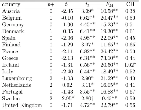
Table 8 shows the results of HEGY tests on the beef price series. Again, seasonal unit roots are usually rejected, while the unit root at one appears to be supported. The countries where the rejection of the seasonal unit root is least convincing are Sweden, Austria, Netherlands, and Luxembourg. We note, however, that the Swedish series is rather short and that it is the only one where the unit root at one is not supported at the 5% signi…cance level.

10

Table 6: HEGY tests for seasonal unit roots in the soft wheat price series.

country p+ t

t

F

CH

Austria 0 -1.87 1.69 0.66 0.77

Belgium 1 -1.94 5.33* 15.94** 0.79

Germany 0 -1.63 3.75** 13.06** 0.49 Denmark 2 -1.52 6.07** 51.84** 0.93 y

Spain 1 -1.13 8.11** 41.79** 0.53

Finland 0 -0.86 3.57** 16.39** 0.96 y

France 1 -2.37 4.08** 6.45 y 1.09*

Italy 2 -2.41 3.18* 18.14** 1.17*

Netherlands 0 -1.44 5.82** 47.20** 0.91 y Portugal 0 -1.42 3.13* 11.61** 0.51

Sweden 0 -1.96 4.45** 13.21** 0.42

United Kingdom 1 -2.48 8.58** 47.67** 0.25

Note: y denotes signi…cance at the 10% level, * at the 5% level, and ** at the 1% level.

Table 7: HEGY tests for seasonal unit roots in the durum wheat price series.

country p+ t

t

F

CH

Austria 1 -1.48 3.42** 14.39** 0.49 Spain 1 -0.48 5.77** 40.15** 0.23 France 2 -2.26 3.73** 22.97** 0.41 Italy 2 -1.59 3.96** 26.69** 0.66

Note: y denotes signi…cance at the 10% level, * at the 5% level, and ** at the 1% level. t

, t

, and F

are the HEGY test statistics for unit roots at +1, -1, and I. CH denotes the Canova-Hansen test statistic.

11

Table 8: HEGY tests for seasonal unit roots in the beef price series.

country p+ t

t

F

CH

Austria 0 -2.35 3.09* 10.58** 0.38

Belgium 1 -0.10 6.62** 20.47** 0.50

Germany 0 -1.30 4.45** 15.23** 0.51

Denmark 1 -0.35 6.41** 19.30** 0.61

Spain 0 -2.06 4.98** 22.09** 0.45

Finland 0 -1.29 3.07* 11.65** 0.65

France 0 -2.11 6.82** 26.42** 0.50

Greece 0 -2.13 6.34** 73.10** 0.44

Ireland 0 -1.31 6.56** 20.56** 1.02*

Italy 0 -2.40 6.44** 18.49** 0.52

Luxembourg 2 -1.03 2.90* 21.29** 0.40 Netherlands 2 0.02 3.11* 16.05** 0.41 Portugal 0 -1.43 3.55** 16.88** 0.67

Sweden 2 -2.95* 2.80 y 9.45** 0.59

United Kingdom 0 -1.71 4.72** 22.79** 0.56

Note: y denotes signi…cance at the 10% level, * at the 5% level, and ** at the 1% level. t

, t

, and F

are the HEGY test statistics for unit roots at +1, -1, and I. CH denotes the Canova-Hansen test statistic.

12

Figure 2: Time series plot of logarithmic barley prices.

4 Multivariate evidence

Visual inspection of time-series graphs (see, for example, Figure 2) and com- mon sense suggests that prices for the same food item in various countries should be cointegrated because of the Common Agricultural Policy, and if one accepts that these variables are individually …rst-order integrated (I(1)).

Heterogeneity of commodities and transportation costs, however, may be obstacles to the naive adoption of a ‘law of one price’. Therefore, such coin- tegrating laws may contain a non-zero constant for logarithmic prices that re‡ects a time-constant relative di¤erence. Unfortunately, such cointegrating relationships are hard to establish on statistical grounds, due to the shortness of the time series.

For example, a four-variables system consisting of the (logarithmic) du- rum wheat price series with exogenous seasonal constants does not permit cointegration testing at all, while the null hypothesis of non-cointegration cannot be rejected in a three-variables system that excludes Austria. Only if the dimension is reduced to two and one focuses solely on Italy and France, does statistical evidence on one cointegrating vector clearly emerge. It ap- pears that French prices error-correct to di¤erences between French and Ital- ian prices, while Italian prices do not react to French prices. Unfortunately, such interesting results cannot be established for larger price systems.

13

For the purpose of exploring common factors in seasonal price cycles, we prefer to allow for the possibility of cointegration, with cointegrating vectors de…ned by di¤erences across countries. We note that models using lagged inter-country di¤erences as additional regressors are more general than vector autoregressions in …rst di¤erences. Excluding potential error-correction may be more harmful for exploring the seasonal part than adding them spuriously.

The systems that we have in mind are of the form y

= + Ad

+

y

+

X

j=1

j

y

+ "

; (2) where y is the n–dimensional vector of logarithmic price variables, d denotes (any three out of four) quarterly dummy variables, is a cointegrating matrix of dimension (n 1) n, describes the intensity of adjustment to inter- country di¤erences, p is a lag order, and " denotes the white-noise errors.

We generally found low lag orders to be su¢ cient for whitening the error process— see the low lag orders for the univariate HEGY tests that were identi…ed by AIC— and hence we retain the value of p = 1 that is prescribed by multivariate information criteria.

We again note that the size of our samples does not permit reliable de- cisions on the cointegrating rank of the vector autoregression but also that keeping the possibly spurious regressors in y

still yields a consistent es- timator for the system parameters. For forecasting, the situation should be assessed once more, however, as the presence of small and statistically insigni…cant coe¢ cients in tends to deteriorate forecasting performance.

As our main focus is on the seasonal structures, we consider rank restric- tions on the seasonal matrix A. If s common factors are present in the panel of price series, the rank of A will be s < 3. The estimation of a VAR model with two rank-restricted matrices requires special econometric methods. The speci…cation of a cointegrating matrix simpli…es this problem considerably.

In fact, estimation of the model with pre-speci…ed and given rank s can be conducted e¢ ciently by the usual reduced-rank regression algorithm (see Anderson 1951, Tso 1981).

The validity of rank restrictions can be tested using a usual restriction statistic that compares the unrestricted model and the restricted model with seasonal common features. Variants of such statistics are the F–statistic, which is often reported in linear regressions, and the Fisher statistic

F = n

^

^

^

;

where the ^

denote ML estimates of the error variances from the unrestricted and unrestricted models and n

is the degrees of freedom of the denominator.

14

In the present case, n

= (T 3 2N )N , if T is the sample size and N is the number of individuals.

Franses and Kunst (2005) employed a similar statistic in an investi- gation of convergence of seasonal cycles in European industrial production.

They suggest monitoring convergence by computing the statistic on moving windows. We follow their suggestion and consider windows of size T = 40, i.e.

of 10 years. In an application of this monitoring idea to the barley series, we restrict the number of countries to …ve: Belgium, Denmark, France, Spain, and the United Kingdom. These …ve countries permit using an acceptable common time range of 1975:3 to 2001:4.

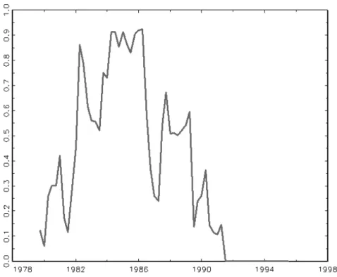
We obtain the image in Figure 3. Instead of the series of Fisher test statis- tics, we show p–values based on the asymptotic chi-square null distribution with 2(N 1) degrees of freedom. The graph shows that a common sea- sonal cycle emerged around 1980 but disappeared again in the 1990s, when p–values fell below the 0.05 signi…cance mark. If the Dutch barley prices are included, the graph is similar but the drop in the p–value occurs somewhat earlier, which indicates that the Dutch seasonal cycle has diverged from other countries in the late 1980s already.

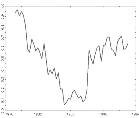
In contrast, the results for soft wheat prices are more supportive of a common seasonal cycle. For this crop, we selected …ve countries— Belgium, France, Italy, the Netherlands, and the United Kingdom— for which series were available for a common time range covering 1971:1–2000:2. The window length had to be increased to 60 observations, as the 40-quarters version turned out to be too volatile. Figure 4 demonstrates that a common cycle cannot be rejected for most of the time. In the 1980s, evidence in favor of a common cycle turned out to be slightly weaker but the p–value re-increased quickly to the acceptance region in the sequel. The overall impression from the monitoring graph suggests keeping the restriction for forecasting, as for that purpose the behavior toward the end of the sample is most important.

For durum wheat, the available sample size is very short, and so is the set of usable country data. We conducted a tentative testing experiment for a three-variables set that contains Spain, France, and Italy for the years 1985–2000. While the end of the sample is more favorable to the existence of a common seasonal cycle, with the implied p–value increasing to 7%, the main impression is that a common cycle has to be rejected.

Beef prices yield comparable results. Again, the series are short, start- ing as late as 1985 for eight countries: Belgium, Denmark, France, Greece, Ireland, Italy, Luxembourg, and the Netherlands. A common seasonal cycle is rejected for the earlier years but it tends to be accepted after 1992. As we reported above, this variables shows less seasonal variation than the …eld crops, hence we omit a detailed analysis.

15

Figure 3: Testing for a common seasonal cycle in barley prices. Countries in the sample are Belgium, Denmark, France, Spain, and the United Kingdom.

Graph shows p–values for the relevant test statistic.

16

Figure 4: Testing for a common seasonal cycle in soft wheat prices. Countries in the sample are Belgium, France, Italy, the Netherlands, and the United Kingdom. Graph shows p–values for the relevant test statistic.

17

5 Forecasting

Basically, we wish to forecast agricultural commodity price series in country panels. While it may be interesting to exploit information across di¤erent farm products, we assume that the impact on forecast precision would be mi- nor. Furthermore, we wish to base our forecasts on the structure of the vector autoregressive model (2). It is known that forecast precision can be impaired by keeping parameters in prediction models that have low statistical signif- icance or are numerically small, particularly if estimates of such parameters are critically a¤ected by outliers or are subject to slow change over time. As a result, we consider an unrestricted version of the basic model but also re- stricted versions with less parameters and more degrees of freedom. Among the possible restrictions, we focus on common factors in seasonal cycles and on omitting the error-correction terms, which have some basis in economic plausibility and visual impression but much less so in statistical tests.

5.1 Missing values and interpolation

In the analysis of the country panels, a main obstacle is the heterogeneity in the time ranges of available data. Some country series start at later dates, often but not always in accord with later accession to the European Union.

Other country series are not available after certain dates, presumably because of longer lags in reporting price observations. Again other country series are available for speci…c seasons only. These latter cases will be excluded from further analysis.

For countries with a later sample start, we consider the following proce- dure. Because it is not possible to reach reliable statistical decisions with regard to hypotheses such as the nature of seasonal cycles, we tentatively assume that the basic characteristics of the multivariate systems are not af- fected by additional countries. Even under the assumption of constant basic model structure, it is still di¢ cult to get reliable parameter estimates. Using estimates from a period of maximal data availability only, such as from the mid-1990s onward, would incur a regrettable loss in the accuracy of estimates for core series, where longer time ranges are available. Therefore, parameters estimated from such short samples should only be considered for countries with late starting points. While this results in an asymmetry of the predic- tion model and maybe in a causal ordering that is at odds with facts, such as in cases where important countries joined later, we feel this solution to be preferable to possible alternatives.

As a …rst example, consider the barley series. Figure 2 summarizes the

…ve countries that are available for samples of reasonable length: Belgium,

18

Denmark, France, Spain, and the United Kingdom. While Belgian data end in early 2003 and French data at the end of 2001, an attractive set of countries has data for more recent years: Austria, Germany, Finland, and Sweden. In contrast, data for Italy, Greece, Portugal and the Netherlands are not available for recent and continuous time periods. The latter set will be ignored in the following, and attention will focus on nine countries. We have found that the …ve basic countries do not share a common seasonal cycle, and we assume that the four remaining cases will not modify this …nding. While this assumption is supported by a naive interpretation of the evidence, as collecting more cases cannot establish common structure that was not even found in the smaller set, this is not necessarily due for evidence based on statistical signi…cance. For the joining set of four countries, price changes are modeled as depending on own lags, cross lags in the new set, and cross lags from the old set. In contrast, price changes in the United Kingdom will not be modeled as depending on German lags, for example.

Regarding the problem of missing data at the end of the sample, these were interpolated by model-based predictions. To this end, several options are conceivable. First, one may replace the unknown observation at time t by its implied conditional expectation based on estimates for the time range ending at t 1. Alternatively, one may consider using the information in- cluding t and later observations fully, for parameter estimation as well as for calculating conditional expectations. This would be justi…ed if other se- ries access past values of the missing variable and if the forecasting period for the whole system starts at t + h with h > 1. For technical reasons, we will not use any back-casting steps, and we will treat the interpolated val- ues just like observations, with the exception that they will not be used for forecasting evaluations. We will, however, use the correlation across errors in constructing the value at t.

To permit a formal exposition, consider two series X and Y in a vector- autoregressive scheme

(X

; Y

)

= A(X

; Y

)

+ e

;

where X is only observed for t < s. The unknown X

is replaced by E(X ^

j X

; t < s; Y

; t s), where the model-based approximation to con- ditional expectation E ^ is estimated using observations for X

; t < s; Y

; t < s.

This yields an arti…cial series of values X

; X

; : : :, which are then re- garded as observations for future prediction including updating of parameter estimates. In order to calculate the conditional expectation with regard to the contemporaneous value Y

, the estimate of the error-covariance ma- trix Ee

e

is subjected to a Choleski factorization, which allows to represent

19

E(X ^

j X

; t < s; Y

; t s) in regression form. Using E(X ^

j X

; t < s; Y

; t <

s)) = ^ A(X

; Y

)

instead would entail some internal consistency, if corre- lation across series were strong.

The formal expression for E(X

j X

; t < s; Y

; t s) permits an attrac- tive interpretation. Assume that the remaining variables of the system Y have dimension n 1. Then, re-order the series so that the predicted scalar variable X comes last. Further, normalize the last row of the inverted left Choleski factor by dividing through the (n; n)-element, such that the row corresponds to a Choleski-style decomposition of the form LDL

instead of LL

. Finally, let us denote this (n 1)-row vector without the 1–element at position (n; n) as l

. Then, it can be shown that

E(X

j X

; t < s; Y

; t s) = E(X

j X

; t < s; Y

; t < s)

+l

(E f Y

j X

; t < s; Y

; t < s) Y

g ; (3) which can be interpreted as follows. The …rst-round prediction of X

is corrected when contemporaneous values Y

become observable, with weights depending on error correlation.

For example, in the barley data set this method was used to construct

…ve additional values for Belgium and ten additional values for France, such that …nally a full data set ending in 2004:2 was obtained.

5.2 Forecasting the barley price series

While the statistical in-sample evaluation presented in the Sections 3 and 4 yields no evidence on cointegration across countries and hardly any evi- dence on a common seasonal cycle, we conduct a comparative evaluation of forecasting performance over the end of the sample.

In this way, we deviate from the traditional modelling paradigm that keeps only statistically validated models. It may well be that models rejected in-sample on statistical grounds dominate others that pass diagnostic checks, in particular with regard to the end of the sample, which in turn is the most important part for assessing the future beyond the current sample end. For a related, recent discussion on methodological issues, see Granger (2005).

The core model contains …ve countries: Belgium, Denmark, Spain, France, and United Kingdom. This set allows a homogeneous starting point in 1975.

Unfortunately, information on Italy stops after the second quarter of 2000, such that it had to be excluded from further investigation. For Belgium and France, the missing time span at the end is considerably shorter, hence these two countries were interpolated as described above. These interpolated values are not used in evaluating predictive accuracy.

20

As reported above, the statistical in-sample evaluation does not support cointegration across countries and hardly supports the existence of a common seasonal cycle. Assuming cointegration across countries or not, and assuming a common seasonal cycle or not yields four di¤erent prediction models. Table 9 shows root mean squared errors (RMSE) and mean absolute errors (MAE) for all four models in the ‘horse race’, with separate …gures for the core and the added series. Forecasts are single-step for the last ten observations (two and a half years) of the sample. All used coe¢ cient estimates are calculated using the past only, therefore all predictions are truly out-of-sample.

Table 9: Forecasting performance for the barley price series.

model CS model CS-EC basic model model EC MSE

core series 0.0433* 0.0457 0.0446 0.0464

added series 0.0421* 0.0491 0.0482 0.0563 MAE

core series 0.0365* 0.0376 0.0374 0.0389

added series 0.0341* 0.0408 0.0385 0.0470 Note: core series are Belgium, Denmark, Spain, France, and the United Kingdom; added series are Austria, Germany, Finland, and Sweden.

Contrary to the previously reported statistical evidence, the clear winner of our forecasting contest is the most parsimonious structure that assumes no error-correction terms and imposes a reduced rank on the seasonal cycle matrix. Superior performance of parsimonious models, even when restrictions are rejected on a usual statistical signi…cance level, is not uncommon in forecasting experiments.

5.3 Forecasting the wheat price series

While the statistical in-sample evaluation presented in the Sections 3 and 4 yields no evidence on cointegration across countries and evidence on a common seasonal cycle remains sensitive to variations over time, we again conduct a comparative evaluation of forecasting performance over the end of the sample.

For soft wheat, the core model contains …ve countries: Belgium, France, Italy, Netherlands, and United Kingdom. This set permits a homogeneous starting point in 1971. Information on Italy stops after the second quarter of 2002— that is, two years later than for the barley prices— after which the

21

Italian price is interpolated using current and past values of all series, as it was outlined in Subsection 5.1. These interpolated values are not used in evaluating predictive accuracy.

To the core series, three more countries (Denmark, Spain, Sweden) are added, where data start at later time points. These added series are predicted using the full set, while the added set is not used in forecasting the core set, where longer and more reliable samples permit coe¢ cient estimation with greater accuracy.

Table 10: Forecasting performance for the soft wheat price series.

model CS model CS-EC basic model model EC MSE

core series 0.0325 0.0429 0.0323* 0.0520

added series 0.0369 0.0574 0.0358* 0.0519 MAE

core series 0.0245 0.0319 0.0243* 0.0352

added series 0.0290* 0.0437 0.0291 0.0418 Note: core series are Belgium, France, Italy, Netherlands, and United King- dom; added series are Denmark, Spain, and Sweden.

Table 10 clearly demonstrates that assuming cointegration across coun- tries is detrimental for prediction. This does not necessarily imply that price levels of di¤erent countries are free to drift apart in the long run. Simula- tion experiments have been reported in the literature that, even for a model structure known to be cointegrated, forecasting only improves after ten steps or more (see Engle and Yoo, 1987). It is also possible that convergence of price levels plays a role, which, being a non-linear process with gradual changes in equilibria, would lead to statistical evidence against cointegration in …nite samples.

Table 10 is less clear with respect to common seasonal cycles. The rank restriction on the seasonal matrix together with cointegration yields the worst performance, while without cointegration summary results are more or less on a par for the speci…cations with and without the rank restriction.

For the durum wheat series, we obtain the results that are summarized in Table 11. After 2000:3, the Italian series had to be extrapolated, and a similar action was performed on the Portuguese data that is available for disconnected quarters only in the most recent years.

Table 11 shows that the model with common seasonal cycles clearly dom- inates all competing structures. In contrast, adding error-correction terms

22

Table 11: Forecasting performance for the durum wheat price series.

model CS model CS-EC basic model model EC MSE

core series 0.0480* 0.0752 0.0595 0.0564

added series 0.0479* 0.2558 0.0518 0.0720 MAE

core series 0.0360* 0.0627 0.0443 0.0447

added series 0.0322* 0.1151 0.0380 0.0539 Note: core series are France and Italy; added series are Austria, Spain, and Portugal.

to the simplest model implies an unstable vector autoregression and leads to the worst predictions. The comparatively small system dimension of n = 5 implies that the assumed common seasonal structure imposes a less severe constraint on the model than for the much larger soft-wheat system. This may partly be responsible for the divergence in results for the two species of wheat.

In summary, common seasonality helps in predicting the durum wheat prices— just like the barley prices— while the seasonal cycle in the case of soft wheat prices is more heterogeneous across European countries.

5.4 Forecasting the beef price series

From Section 4, it is known that the statistical evidence supports a restric- tion of common seasonal cycles in the beef price series toward the end of the sample, which is the most important part of the sample for forecast- ing. Therefore, it is not surprising that Table 12 shows that the model with common seasonality yields the most precise predictions.

6 Summary and conclusion

The comparison between model selection based on statistical in-sample cri- teria and the ranking of the very same models on the basis of out-of-sample prediction evaluation often yields con‡icting preferences. Typically, highly simpli…ed structures imply the best forecasting performance, even when the simpli…cation is not supported by statistical tests. The most likely reason is that comparatively pro‡igate models require the estimation of additional

23

Table 12: Forecasting performance for the beef price series.

model CS model CS-EC basic model model EC MSE

core series 0.0221* 0.0258 0.0250 0.0276

added series 0.0248* 0.0384 0.0267 0.0401 MAE

core series 0.0159* 0.0184 0.0193 0.0216

added series 0.0201* 0.0267 0.0217 0.0280 Note: core series are Belgium, Denmark, France, Greece, Ireland, Italy, Lux- embourg, and Netherlands; added series are Germany, Spain, Portugal, and United Kingdom.

parameters. These estimates are subject to sampling variation and lead to a deterioration of predictions that implicitly use them as true values.

The examples on cross-country panels of European agricultural prices is well in line with this pattern. While individual series are subject to often sizeable seasonal patterns with many idiosyncratic features, as climate and traditions vary strongly across Europe, assuming a single European seasonal cycle improves prediction for three out of four agricultural products. Only for soft wheat, where a larger set of countries is available, does the ranking of forecasts correspond to the statistical rejection of a common seasonal cycle.

In contrast, the lack of statistical support for cointegration among country series is re‡ected fully in the prediction experiments. While economic theory may support ‘laws of one price’for price variables of di¤erent countries that are subject to the EU common agricultural policy, there is little evidence on parallel price movements in our series. Constructing forecast models on the plausible, although statistically rejected, error correction idea sometimes even leads to unstable models and to forecast failure.

Acknowledgements

We wish to thank Jose Luis Gallego for helpful comments on an earlier ver- sion. The usual proviso applies.

24

References

[1] Anderson, T.W. (1951) ‘Estimating linear restrictions on regression coe¢ cients for multivariate normal distributions.’Annals of Mathemat- ical Statistics 22, 327–351.

[2] Canova, F., and B.E. Hansen (1995) ‘Are Seasonal Patterns Con- stant over Time? A Test for Seasonal Stability,’Journal of Business &

Economic Statistics 13, 237–252.

[3] Engle, R.F., and Yoo, B.S. (1987) ‘Forecasting and Testing in Co- integrated Systems’. Journal of Econometrics 35, 143–159.

[4] Franses, P.H.F., Kunst, R.M. (2005) ‘Analyzing a panel of seasonal time series: Does seasonality converge across Europe?’ Mimeo, Institute for Advanced Studies, Vienna.

[5] Friedman, M. (1962) ‘The interpolation of time series by related se- ries’. Journal of the American Statistical Association 57, 729–757.

[6] Ghysels, E., and Osborn, D.R. (2001) The Econometric Analysis of Seasonal Time Series. Cambridge University Press.

[7] Granger, C.W.J. (2005) ‘Modeling, Evaluation, and Methodology in the New Century,’Economic Inquiry 43, 1–12.

[8] Hylleberg, S., Engle, R.F., Granger, C.W.J., Yoo, B.S. (1990)

‘Seasonal Integration and Cointegration,’ Journal of Econometrics 44, 215–238.

[9] Hylleberg, S, (1995) Tests for Seasonal Unit Roots: General to Spe- ci…c or Speci…c to General?, Journal of Econometrics 69, 5–25.

[10] Johansen, S. (1988) ‘Statistical analysis of cointegration vectors’Jour- nal of Economic Dynamics and Control 12, 231–254.

[11] Johansen, S. (1995) Likelihood-Based Inference in Cointegrated Vector Autoregressive Models. Oxford University Press.

[12] Kunst, R.M. (1993) ‘Seasonal Cointegration, Common Seasonals, and Forecasting Seasonal Series,’Empirical Economics 18, 761–776.

[13] Kunst, R.M., and M. Reutter (2002) ‘Decisions on seasonal unit roots’. Journal of Statistical Computation and Simulation. 72, 403–418.

25

[14] Miron, J.A. (1996) The Economics of Seasonal Cycles. MIT Press.

[15] Palaskas, T., and T.J. Crowe (1996) ‘Testing for price transmis- sion with seasonally integrated producer and consumer price series from agriculture’European Review of Agricultural Economics 23, 473–486.

[16] Sargent, T. (2001) Foreword to: Ghysels, E., and Osborn, D.R.

The Econometric Analysis of Seasonal Time Series. Cambridge Univer- sity Press.

[17] Tso, M.K-S. (1981) ‘Reduced-rank regression and canonical analysis.’

Journal of the Royal Statistical Society B 43, 183–189.

26

Authors: Adusei Jumah, Robert M. Kunst

Title: Seasonal Cycles in European Agricultural Commodity Prices Reihe Ökonomie / Economics Series 192

Editor: Robert M. Kunst (Econometrics)

Associate Editors: Walter Fisher (Macroeconomics), Klaus Ritzberger (Microeconomics)

ISSN: 1605-7996

© 2006 by the Department of Economics and Finance, Institute for Advanced Studies (IHS),

Stumpergasse 56, A-1060 Vienna • +43 1 59991-0 • Fax +43 1 59991-555 • http://www.ihs.ac.at

ISSN: 1605-7996