Complexity Theory

(1)

Complexity Theory

Lecture Notes October 27, 2016

Prof. Dr. Roland Meyer

TU Braunschweig

Winter Term 2016/2017

(2)

Preface

These are the lecture notes accompanying the course Complexity Theory taught at TU Braunschweig. As of October 27, 2016, the notes cover 11 out of 28 lectures. The handwritten notes on the missing lectures can be found athttp://concurrency.cs.uni-kl.de. The present document is work in progress and comes with neither a guarantee of completeness wrt. the content of the classes nor a guarantee of correctness. In case you spot a bug, please send a mail toroland.meyer@tu-braunschweig.de.

Peter Chini, Judith Stengel, Sebastian Muskalla, and Prakash Saivasan helped turning initial handwritten notes into L^ATEX, provided valuable feed- back, and came up with interesting exercises. I am grateful for their help!

Enjoy the study!

Roland Meyer

(3)

Introduction

Complexity Theory has two main goals:

• Study computational models and programming constructs in order to understand their power and limitations.

• Study computational problems and their inherent complexity. Com- plexity usually means time and space requirements (on a particular model). It can also be defined by other measurements, like random- ness, number of alternations, or circuit size. Interestingly, an important observation of computational complexity is that the precise model is not important. The classes of problems are robust against changes in the model.

Background:

• The theory of computability goes back to Presburger, G¨odel, Church, Turing, Post, Kleene (first half of the 20^th century).

It gives us methods to decide whether a problem can be computed (decided by a machine) at all. Many models have been proven as powerful as Turing machines, for example while-programs or C-programs. The ChurchTuring conjecture formalizes the belief that there is no notion of computability that is more powerful than computability defined by Turing machines. Phrased positively, Turing machines indeed capture the idea of computability.

• Complexity theory goes back to ”On the computation complexity of algorithms” by Hartmanis and Stearns in 1965 [?]. This paper uses multi-tape Turing machines, but already argues that concepts apply to any reasonable model of computation.

(4)

Crossing Sequences and

Unconditional Lower Bounds

Goal: We establish an unconditional lower bound on the power of a uni- form complexity class.

• The termunconditional is best explained by its opposite. If we show a conditional lower bound — say NP-hardness — we mean that the problem is hardunder the assumption thatP6=NP. An unconditional lower bound does not need such an assumption. Unconditional lower bounds are rare, even proving SAT6∈DTIME(n³) seems out of reach.

• Uniformity means that we use one algorithm (one Turing Machine) to solve the problem for all inputs. Non-uniformmodels may use different algorithms (popular in circuit complexity) for different instances.

To get the desired lower bound, we employ a counting technique called crossing sequences. Crossing sequences are vaguely related to fooling sets in automata theory.

1.1 Crossing Sequences

Let COPY ={w#w|w∈ {a, b}^∗}. This language is not context free and hence not regular.

Goal 1.1. Show an upper and a lower bound for COPY:

• Upper bound: COPY can be decided in quadratic time.

• Lower bound: COPY cannot be decided in subquadratic time (on a 1-tape DTM (deterministic Turing machine)).

(7)

Recall 1.2. 1. When we refer to a problem written as a set, deciding the problem means deciding membership for that set. Given x ∈ {a, b}^∗, does x∈COPY hold?

2. We assume that all tapes of a Turing machine are right-infinite: To the left, they are marked by $. From this marker, one can only move to the right and $ cannot be overwritten. Unless otherwise stated, we will assume that the TM only halts on $.

3. The time and the space requirements of a TM are measured relative to the size of the input. Without further mentioning, this size will be referred to asn.

4. O-notation =asymptotic upper bound (≤, read as no more than):

O(g(n)) :={f :N→N| ∃c∈R+ ∃n₀∈N∀n≥n₀:f(n)≤c·g(n)}. o-notation =asymptotic strict upper bound (<, read asless than):

o(g(n)) :={f :N→N| ∀c∈R+ ∃n₀∈N∀n≥n0:f(n)≤c·g(n)} . Lemma 1.3. COPY ∈DTIME(n²).

The proof is left as an exercise to the reader.

Definition 1.4. Thecrossing sequence ofM on inputx at positioniis the sequence of states of M when moving its head from cell i to cell i+ 1 or from cell i+ 1 to cell i. To be precise, we mean the state that is reached after the transition. We denote the crossing sequence byCS(x, i).

Picture missing If q is a state in an odd position of the crossing sequence, thenM moves its head from left to right. If it is a state in an even position, M moves from right to left. Transitions staying in cell i do not contribute to the crossing sequence.

Lemma 1.5 (Mixing Lemma). Consider wordsx=x₁.x₂ and y=y₁.y₂. If CS(x,|x₁|) =CS(y,|y₁|), then

x₁.x₂ ∈L(M) if and only if x₁.y₂ ∈L(M).

Sketch. Intuitively, the crossing sequence is all thatM remembers aboutx2

resp. y₂ when operating on the left partx₁. Since the crossing sequences are assumed to coincide,M will behave the same onx₁, independent of whether x2 ory2 is on the right. Since the $ symbol (on which we accept) is on the left, we are done.

The next lemma states that the crossing sequences (their length) form a lower bound on the time complexity of a TM. If the TM is guaranteed to move on every transition, even equality holds. The proof is immediate by the definition of crossing sequences.

(8)

Lemma 1.6 (Fundamental Inequality). Time_M(x)≥P

i≥0|CS(x, i)|.

We are now prepared to show the unconditional lower bound.

Theorem 1.7. COPY 6∈DTIME(o(n²)).

Proof. LetM be a 1-tape DTM for COPY. Consider inputs of the form w₁.w₂#w₁.w₂ with |w₁|=|w₂|=n.

We have:

X

w2∈{a,b}ⁿ

TimeM(w1.w2#w1.w2)

( Lemma 1.6 ) ≥ X

w2∈{a,b}ⁿ 3n

X

ν=2n+1

|CS(w1.w2#w1.w2, ν)| (1.1)

=

3n

X

ν=2n+1

X

w2∈{a,b}ⁿ

|CS(w1.w2#w1.w2, ν)|. (1.2) Considerν with 2n+ 1≤ν ≤3n. Denote the average length of the crossing sequences from the setCrossν :={CS(w1.w2#w1.w2, ν)|w2 ∈ {a, b}ⁿ}by

lν :=

P

w2∈{a,b}ⁿ|CS(w1.w2#w1.w2, ν)|

2ⁿ .

Claim 1.8. At least half (which means ²₂ⁿ = 2ⁿ⁻¹) of the crossing sequences fromCrossν have length≤2lν.

Claim 1.9. The crossing sequences fromCross_ν are pairwise distinct.

Claim 1.10. The number of crossing sequences of length≤2l_ν is bounded by (|Q|+ 1)^2l^ν, where Qis the set of states ofM.

We add +1 because the sequence may be shorter.

By Claim 1.8 to Claim 1.10, we have

(|Q|+ 1)^2l^ν ≥2ⁿ⁻¹ .

Note that we need the fact that the crossing sequences are different to enforce the inequality. Since

(|Q|+ 1)^2l^ν = (2^log(|Q|+1))^2l^ν = 2log(|Q|+1)2lν ,

monotonicity of logarithms yields log(|Q|+ 1)2lν ≥n−1. Hence, there is a constantc(depending on Qbut not depending on nand not on ν) so that

lν ≥ cn . (1.3)

With this lower bound,

(9)

Claim 1.11. P

w2∈{a,b}ⁿTime_M(w₁.w₂#w₁.w₂)≥2ⁿcn² . Since there are only 2ⁿ words w2, Claim 1.11 implies

Time_M(w₁.w₂#w₁.w₂)≥cn²

for all least onew2. This concludes the proof of Theorem 1.7.

Claim 1.8 is the following statement.

Lemma 1.12. If ¹_nPn

i=1w_i=d, at least half of the w_i have a value ≤2d.

Proof. Assume at least half of thewi have a value >2d. Then

n

X

i=1

wi > n

2 ·2d=nd . From this we can deduce

1 n

n

X

i=1

w_i > nd n =d . This contradicts the assumption.

Proof of Claim 1.9. Towards a contradiction, consider two words u 6= v of length |u| = |v| = n and assume CS(w1.u#w1.u, ν) = CS(w1.v#w1.v, ν).

Recall that 2n+ 1≤ν≤3n. By Lemma 1.5, we have

w1.u#w1.u∈L(M) iff w1.u#w1.v∈L(M) .

Since the former word is a member ofCOPY but the latter is not, and since M is assumed to acceptCOPY, this is a contradiction.

Proof of Claim 1.11.

X

w2∈{a,b}ⁿ

Time_M(w₁.w₂#w₁.w₂)

( (In)equalities (1.1) and (1.2) ) ≥

3n

X

ν=2n+1

X

w2∈{a,b}ⁿ

|CS(w1.w2#w1.w2, ν)|

( Definition lν ) =

3n

X

ν=2n+1

2ⁿlν

( Inequality (1.3) ) ≥

3n

X

ν=2n+1

2ⁿcn

= 2ⁿcn² .

(10)

1.2 A Gap Theorem for Deterministic Space Com- plexity

Recall that the input tape of a space-bounded TM is read only. The TM can only write to (and read from) its work tape. Ifs(n) :N→Nis a space bound for the work tape, we will assumes(n)>0 for all n∈N. The reason is that we need a position for the head. The functions(n) isunbounded if for allm∈Nthere is ann∈Nso thatm < s(n). Note thats(n) is unbounded if and only ifs(n)∈ O(1)./

Goal 1.13. Show that o(loglog(n)) work tape is no better than having no tape at all.

Theorem 1.14. DSPACE(o(loglog(n))) =DSPACE(O(1)).

The inclusion from right to left is left as an exercise to the reader. We will prove the reverse inclusion.

Definition 1.15. Consider a TM M = (Q,Σ,Γ,$, , δ, q₀, q_acc, q_rej) (the precise definition will be given in Section 2.1). Asmall configuration of M consists of:

• the current state (inQ),

• the content of the work tape (in Γ^∗), and

• the head position on the work tape.

The small configuration omits the input word and the head position on the input tape.

Definition 1.16. The extended crossing sequence ofM on input x at posi- tioni,ECS(x, i), is the sequence of small configurations ofM when moving its head from celli toi+ 1 or from cell i+ 1 toion the input tape.

Lemma 1.17. LetM bes(n)-space bounded. The number of extended crossing sequences on inputs of lengthn is at most 2²^ds(n), where d is a constant (depending on M but not on the input).

Proof. LetM = (Q,Σ,Γ,$, , δ, q0, qacc, qrej) be thes(n)-space-bounded TM of interest. The number of small configurations on inputs of length n is bounded by|Q| |Γ|^s(n)s(n). Since s(n)>0, we have

|Q| |Γ|^s(n)s(n)≤c^s(n),

wherec is a constant depending only onQand Γ but not on n.

(11)

In an extended crossing sequence, no small configuration may appear twice in the same direction. Otherwise, a (large) configuration ofM would appear twice in the computation. As M is deterministic it would be stuck in an infinite loop. SinceM is assumed to halt, this cannot happen. Thus, there are at most

(c^s(n)+ 1)

| {z }

lef t

c^s(n)·(c^s(n)+ 1)

| {z }

right

c^s(n) = (c^s(n)+ 1)^2c^s(n) ≤2²^ds(n)

different extended crossing sequences on inputs of length n, where d >0 is a constant (again dependent onM but not on the input).

Proof of Theorem 1.14. Towards a contradiction, assume there was a lan- guageL∈DSPACE(o(loglog(n))) withL /∈DSPACE(O(1)). Then there is a 1-tape DTMM withL=L(M) and space bounds(n)∈o(loglog(n))\O(1).

We will show thatM cannot exist.

Sinces(n)∈o(loglog(n)), there is an n0∈Nso that for alln≥n0 we have s(n)< 1

2dloglog(n) .

Here,dis the constant from Lemma 1.17. With this, we can deduce 2²^ds(n) <2²^d

1 2dloglog(n)

=

2²^loglog(n)¹₂

=n¹² ≤ n

2 . (1.4)

By the fact thats(n) is unbounded, there is an inputx⁰ so that s0 := Space_M(x⁰)>max{s(n)|0≤n≤n0}.

Let x be the shortest input with s₀ = Space_M(x). By the definition of s₀ we have |x|> n0. Otherwise, Space_M(x) =s0 > s(|x|)≥Space_M(x), which is a contradiction.

By Lemma 1.17 and Inequality (1.4), the number of extended crossing sequences is smaller than ^|x|₂ . Hence, there are positionsi < j < k with

ECS(x, i) =ECS(x, j) =ECS(x, k).

Indeed, if there were at most two positions for each extended crossing sequence, we would get|x|<2·^|x|₂ =|x|, which is a contradiction.

Now we shorten the inputx by cutting out either the sequence fromi toj or the sequence from j to k. Since every small configuration on x appears in at least one of the two shortened strings,M will use the same space on at least one of the two strings. This contradicts the choice ofxas the shortest input with space bounds₀.

(12)

The above theorem can be phrased as follows: If M runs in o(loglog(n)) space, then M accepts a regular language.

Theorem 1.18. DSPACE(O(1)) =REG.

The relationship is non-trivial as a space-bounded TM may visit an input symbol arbitrarily often whereas a finite automaton will see it only once.

We conclude the section with an example that complements Theorem 1.14:

Starting fromDSPACE(loglog(n)), we obtain non-regular languages.

Example 1.19. Consider the language

L := {bin(0)# bin(1)#· · ·# bin(n)|n∈N}.

It can be shown thatL is not regular but in DSPACE(loglog(n)). With the Theorems 1.14 and 1.18, we conclude that we cannot do better: Ldoes not lie in DSPACE(o(loglog(n))).

(13)

Chapter 2

Time and Space Complexity Classes

Goal: The goal in this chapter is to introduce the basic complexity classes.

They have proven to be useful because:

• they characterize important problems like computing, searching/guess- ing, playing against an opponent and

• they are robust under reasonable changes to the model: Pis the same class of problems no matter whether we take polynomial-time Tur- ing machines, polynomial-time while programs, polynomial-time RAM machines or polynomial-time C++ programs.

2.1 Turing Machines

Goal 2.1. Define different types of Turing Machines: deterministic TMs, non-deterministic TMs, multi-tape TMs, recognizers and deciders.

Definition 2.2. A deterministic 1-tape Turing machine (TM) is a 9-tuple M = (Q,Σ,Γ,$, , δ, q₀, q_acc, q_rej),

where:

• Qis a finite set ofstates withinitial state q0,accepting state qaccand rejecting state qrej,

• Σ is the finiteinput alphabet not containing nor $,

• Γ is thetape alphabet with Σ⊆Γ. ∈Γ is theblank symbol, $∈Γ is theleft endmarker,

• δ:Q×Γ−→Q×Γ× {L, R} is thetransition function.

(14)

We have the following requirements onM:

• The endmarker is never overwritten:

∀p∈Q∃q ∈Q:δ(p,$) = (q,$, R)

• Once the machine halts, it no longer writes:

∀b∈Γ ∃d, d⁰ :δ(qacc, b) = (qacc, b, d) andδ(qrej, b) = (qrej, b, d⁰) For the semantics of a Turing machine we also define the notion ofconfigu- rations and atransition relation among configurations:

Definition 2.3. LetM = (Q,Σ,Γ,$, , δ, q0, qacc, qrej) be a Turing machine.

a) A configuration of M is a triple u q v ∈ Γ^∗×Q×Γ^∗. The idea behind this notation is thatM’s head is on the first symbol ofv, the machine is in state q and the tape content isuv.

b) Thetransition relation →⊆(Γ^∗×Q×Γ^∗)×(Γ^∗×Q×Γ^∗) is defined by:

u.a q b.v →u q⁰a.c.v, ifδ(q, b) = (q⁰, c, L) u.a q b.v →u.a.c q⁰v, ifδ(q, b) = (q⁰, c, R).

A configuration u q is understood to be equivalent tou q . c) Theinitial configuration of M on inputw∈Σ^∗ is q0$.w.

d) A configuration of the form u qaccv is calledaccepting. Similarly, a configuration of the form u q_rejv is called rejecting.

Accepting and rejecting configurations are also called halting configurations.

e) The Turing machineM accepts input w, if there is a sequence of configurations:

c1 →c2 → · · · →cn,

wherec1 is the initial configuration ofM on inputwandcnis an accepting configuration.

f) Thelanguage of M is defined by:

L(M) :={w∈Σ^∗|M acceptsw}.

Definition 2.4. A language L ⊆Σ^∗ is called (Turing) recognizable or recursively enumerable, ifL=L(M) for some Turing machineM.

Remark 2.5. When a TM is started on an input, there are three possible outcomes:

(15)

1. M may accept, so it reaches an accepting configuration, 2. M may reject, so it reaches a rejecting configuration or 3. M mayloop, which means thatM does not halt.

Hence, M may fail to accept by rejecting or by looping. Distinguishing looping from taking a long time to accept or reject is rather difficult. In Complexity Theory, we are only interested in machines that halt on all inputs, i.e., that never loop. Such machines are called deciders. They are also said to be total.

Definition 2.6. A languageL⊆Σ^∗is called(Turing) decidableorrecursive, ifL=L(M) for a decider M.

Remark 2.7. Amultitape Turing machineis defined like an ordinary Turing machine but with several tapes. Initially, the input is on the first tape and the remaining tapes are empty. The transition function allows reading, writing and moving the head on some or even on all tapes simultaneously.

Formally,δ is a function:

δ:Q×Γ^k −→Q×Γ^k× {L, R, S}^k

Theorem 2.8. For every multitape Turing machine M there is a 1-tape Turing machineM⁰ withL(M) =L(M⁰). Hence, a language is recognizable if and only if some multitape Turing machine recognizes it.

Remark 2.9. A nondeterministic Turing machine (NTM) may, at any point in a computation proceed according to several possibilities. Formally, the transition function takes the form:

δ:Q×Γ−→P(Q×Γ× {L, R})

The computation of a nondeterministic Turing machine is a tree where the branches correspond to different possibilities of the machine. Ifsome branch of the tree leads to an accepting configuration, the machineaccepts the input.

Thelanguage of a NTMM is defined to be:

L(M) :={w∈Σ^∗| some branch ofM started on waccepts} M is called total or adecider if for every input w∈Σ^∗ all branches halt.

Theorem 2.10. For every (total) NTMM there is a (total) DTM M⁰ with L(M) =L(M⁰). Hence, a language is recognizable if and only if some NTM recognizes it. Moreover, a language is decidable if and only if some NTM decides it.

Recall 2.11. Recapitulation of the notions: Decidable and Semidecidable:

(16)

• A propertyP : Σ^∗ −→B is calleddecidable, if {x∈Σ^∗|P(x) = true} is a recursive set. This means there is a total TM that accepts the input strings having property P, and rejects the strings that violate P.

• A property P is called semidecidable, if {x ∈ Σ^∗|P(x) = true} is a recursively enumerable set.

In short, the notions recursive and recursively enumerable apply to sets, while the notionsdecidableandsemidecidable apply to properties. But they are interchangeable:

P is decidable ⇔ {x∈Σ^∗|P(x) = true}is recursive.

Ais recursive ⇔ ”x∈A” is decidable.

P is semidecidable ⇔ {x∈Σ^∗|P(x) = true}is recursively enumerable.

Ais recursively enumerable ⇔ ”x∈A” is semidecidable.

2.2 Time Complexity

Goal 2.12. Define the two basictime complexity classesDTIME_k(t(n)) and NTIME_k(t(n)).

Definition 2.13. Let M be a Turing machine which is potentially nondeterministic and which may have several tapes. Let x ∈ Σ^∗ be an input of M.

a) We define thecomputation time of M on x to be:

TimeM(x) := max (

number of transitions onp

pis a computation path of M on x

)

If M does not halt on some path, we set TimeM(x) :=∞. Note that for a deterministic Turing machine, there is precisely one computation path.

b) Forn∈N, we define the time complexity of M as : TimeM(n) := max{TimeM(x)| |x|=n}

This measures the worst case behavior of M on inputs of lengthn.

c) Lett:N→Nbe some function. We say that M ist-time-bounded (also written t(n)-time-bounded), if TimeM(n)≤t(n) for alln∈N.

Definition 2.14. Lett:N→Nbe a function. Then we set:

DTIMEk(t(n)) :=

( L(M)

M is ak-tape DTM that is a decider and t(n)-time-bounded

)

NTIMEk(t(n)) :=

( L(M)

M is ak-tape NTM that is a decider and t(n)-time-bounded

)

(17)

We also writeDTIME(t(n)) and NTIME(t(n)) if we assume the Turing machine to have one tape.

Note 2.15. Sublinear time is not meaningful for Turing machines that do not have random access to the input. The problem is that the machine cannot read the whole input on the tape:

LetM be a deterministic Turing machine and assume there is ann∈Nso thatM reads at mostn−1 symbols of the inputx, for every xwith|x|=n.

Then there are words a1, . . . , am with|a_i|< n for 1≤i≤m so that:

L(M) =

m

[

i=1

ai.Σ^∗.

2.3 Space Complexity

Goal 2.16. Define the two basic space complexity classes DSPACE_k(s(n)) and NSPACEk(s(n)).

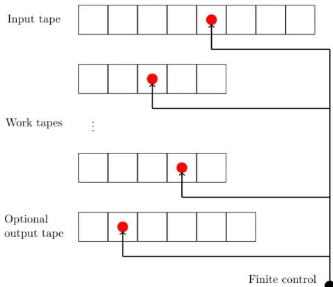
Remark 2.17. Different from the case of time complexity, it is interesting to study computations that run in sublinear space. Therefore, we will assume that a Turing machine has anextra input tape. This tape isread only and not counted towards the consumption of space. An illustration of such a machine is given in Figure 2.1.

Technically, read-only amounts to requiring that wherever the Turing machine reads a symbol, it has to write the same symbol.

Definition 2.18. Let M be a Turing machine which is potentially nondeterministic, which has an additional input tape and which may have several work tapes.

a) Let x ∈ Σ^∗ be an input of M and let c be a configuration of M on x.

Then the space consumption of cis defined by:

Space(c) := max{ |w| |w is a work tape content of c}.

b) Thespace consumption of x is defined to be:

Space_M(x) := max (

Space(c)

cis a configuration that occurs in a computation of M on x

)

If the space grows unboundedly, we set Space_M(x) :=∞.

c) Forn∈N, we define the space complexity of M as:

Space_M(n) := max{Space_M(x)| |x|=n}.

Like for the time complexity, this measures the worst case space consumption of M on inputs of length n.

(18)

Input tape

Work tapes ...

Optional output tape

Finite control states

Figure 2.1: A Turing machine with additional input tape which isread only, several work tapes and an optional output tape. Those machines are used to define the notion ofspace complexity in Definition 2.18. The red dots in the tapes represent the positions of the machine’s heads. These are controlled by a finite number of states.

d) Lets:N→Nbe some function. We say thatM iss-space-bounded (also written s(n)-space-bounded), if Space_M(n)≤s(n) for all n∈N.

Definition 2.19. Lets:N→Nbe a function. Then we define:

DSPACE_k(s(n)) :=





 L(M)

M is ak-tape DTM with extra input tape that is a decider

and s(n)-space-bounded







NSPACE_k(t(n)) :=





 L(M)

M is ak-tape NTM with extra input tape that is a decider

and s(n)-space-bounded





 Example 2.20. Consider the following language:

L={x∈ {a, b}^∗|the number ofas inx equals the number ofbs inx}.

ThenL is in DSPACE(O(logn)).

(19)

Proof. We give a construction of a Turing machine that is O(logn)-space- bounded and that decidesL:

We read the input from left to right. On the work tape, we keep a binary counter. There are two cases:

1. If we read a, we increment (+1) the binary counter.

2. If we read b, we decrement (−1) the binary counter.

We will accept the input if the counter value reached in the end is 0. This clearly decides the languageL. For the space consumption, note the following:

In every step, we store a number ≤ |x| in binary on the work tape. This needs log|x|bits. The construction also requires us to increment and decrement in binary. But this does not cause any space overhead. Hence, the constructed Turing machine needs at mostO(logn) space.

2.4 Common Complexity Classes

Definition 2.21. We now define the common robust complexity classes:

L:=DSPACE(O(logn)) (akaLOGSPACE) NL:=NSPACE(O(logn)) (akaNLOGSPACE)

P:= [

k∈N

DTIME(O(n^k)) (akaPTIME) NP:= [

k∈N

NTIME(O(n^k)) PSPACE:= [

k∈N

DSPACE(O(n^k)) NPSPACE:= [

k∈N

NSPACE(O(n^k)) EXP:= [

k∈N

DTIME

2^O(n^k⁾

(akaEXPTIME) NEXP:= [

k∈N

NTIME

2^O(n^k⁾

(akaNEXPTIME) EXPSPACE:= [

k∈N

DSPACE

2^O(n^k⁾

NEXPSPACE:= [

k∈N

NSPACE

2^O(n^k⁾ .

We will also consider complement complexity classes:

(20)

Definition 2.22. LetC⊆P({0,1}^∗) be a complexity class. Then we define thecomplement complexity class of C to be:

co-C:={L⊆ {0,1}^∗|L∈C where L={0,1}^∗\L}.

Note thatco-C is not the complement ofC, but it contains the complements of the sets inC. Intuitively, a problem inco-C contains the ”no”-instances of a problem inC.

Example 2.23. Consider the following problem:

UNSAT:={ϕ a formula in CNF|ϕis not satisfiable}

ThenUNSAT=SATand sinceSATis a problem inNP, we get thatUNSAT is inco-NP.

Remark 2.24. Goals of Complexity Theory are:

• to understand the aforementioned common complexity classes in more detail. What are the problems they capture ? What do their algorithms look like ?

• to understand the relationship among the classes.

The next theorem is a simple observation that focuses on the second goal:

Theorem 2.25. IfCis a deterministic time or space complexity class, then:

C = co-C. In particular, we have: L = co-L, P = co-P and PSPACE = co-PSPACE.

The proof is left as an exercise.

Definition 2.26. A complexity classC is said to be closed under complement, if for all L∈C we haveL∈C.

Remark 2.27. As a direct consequence of the definition, we get the following equivalences:

C=co-C ⇔C is closed under complement

⇔co-C is closed under complement

Further basic inclusions that focus on the second goal of Remark 2.24 are given in the following lemma:

Lemma 2.28. Let t, s : N → N be two functions. Then these inclusions hold:

DTIME(t(n))⊆NTIME(t(n)) DSPACE(s(n))⊆NSPACE(s(n))

DTIME(t(n))⊆DSPACE(t(n)) NTIME(t(n))⊆NSPACE(t(n)).

(21)

Proof. Since any deterministic Turing machine is also nondeterministic one, the first two inclusions are clear. To prove the latter two inclusions, note that a machine can only scan/write one cell per step. So the tape usage is bounded by the time.

(22)

Chapter 3

Alphabet reduction, Tape reduction, Compression and Speed-up

Goal: We show that the definition of the basic complexity classes isrobust in the sense that it does not depend on the details of the Turing machine definition. These details are the tape alphabet, the number of tapes and constant factors. As a consequence, we do not have to be too accurate about these details. This will simplify proofs a lot.

Technically, we show that a one tape Turing machine with tape alphabet {$, ,0,1} can simulate the other features efficiently.

3.1 Alphabet Reduction

We will use the following notion ofsimulation:

Definition 3.1. Let M and M⁰ be two Turing machines over the input alphabet Σ. ThenM⁰ is said tosimulate M, if ∀x∈Σ^∗ we have: x∈L(M) if and only ifx∈L(M⁰).

Lemma 3.2 (Alphabet Reduction:). Let M = (Q,Σ,Γ,$, , δ, q₀, q_acc, q_rej) be a decider that ist(n)-time bounded. Then there is a decider

M⁰ = (Q,{0,1},{$, ,0,1},$, , δ, q0, qacc, qrej) that is C·log|Γ| ·t(n)-time bounded and for all x∈Σ^∗ we have:

x∈L(M) if and only if bin(x)∈L(M⁰).

Here, bin(−) is a fixed binary encoding for the letters in Γ.

Moreover we have thatM⁰ is deterministic if and only if M is deterministic and that M⁰ has k tapes if and only ifM has k tapes.

(23)

Proof. The Turing machineM⁰will mimic the operations ofM on the binary encoding of the alphabet. To this end, it will:

• use log|Γ| steps to read from each tape the log|Γ| bits encoding a symbol of Γ.

• use its local state to store symbols it has read.

• useM’s transition function/relation to compute the symbols that M writes and the state that M enters.

• store this information in the (control) state ofM⁰.

• use log|Γ|steps to write the encoding into the tapes.

The number of states ofM⁰ is bounded by the number C· |Q| · |Γ|^klog|Γ|.

We get the factor |Q| since we store the states of M, the factor |Γ|^k since M uses ktapes andM⁰ stores the symbols it has read and the factor log|Γ|

for counting from 1 up to log|Γ|.

3.2 Tape Reduction

For the tape reduction, we first show a general construction that we then analyze with respect to its time and space usage.

Theorem 3.3 (Tape Reduction). For every k-tape Turing machine M, there is a one tape Turing machine M⁰ that simulates M. Moreover, M⁰ is deterministic if and only if M is deterministic and if M uses an additional input tape, M⁰ will also use an additional input tape.

Proof. M⁰ simulates one step of M by a sequence of steps. The idea is to storek tapes into one single tape. This tape will be understood as divided into 2k tracks. Technically, the tape alphabet is:

Γ⁰ := (Γ× {∗,−})^k∪Σ∪ {$, }

The (2`−1)-st component of a letter in Γ⁰ stores the content of the `-th tape. The (2`)-th component, which is in {∗,−}, marks the position of the head on the `-th tape by ∗. There is precisely one ∗on the 2`-th track, the remaining symbols are −. For an illustration of the construction, consider Figure 3.1.

A step of M is simulated by M⁰ as follows: M⁰ always starts on the left endmarker $. It moves to the right until it finds the first pure blank symbol . Note that is neither a vector containing nor a vector containing −.

On the way,M⁰ stores thek symbols where the heads ofM point to. Once M⁰ has collected all ksymbols, it can simulate a transition of M. It moves back to the start and, on its way, makes the changes to the tape that M would make. When arriving at $,M⁰ changes the control state.

(24)

. . . ₀ ₀ ₁ ₁ ₀ . . . . . . ₀ ₁ ₀ . . .

... ...

. . . ₀ ₁ ₁ . . .

. . . ₀ ₀ ₁ ₁ ₀ . . . . . . _{− − ∗ − −} . . . . . . ₀ ₁ ₀ . . . . . . _{− − − ∗ −} . . .

... ...

. . . ₀ ₁ ₁ . . . . . . _{− ∗ − − −} . . . Figure 3.1: The different tapes of the Turing machine are combined in one tape with different tracks. The 2`−1-st track keeps the content of tape`, the 2`-th track stores the position of the tape’s head. One symbol in the new tape alphabet is represented by a column in the big tape.

Definition 3.4. Let t, s:N→N be two functions. Define:

DTIMESPACE_k(t, s) :=





 L(M)

M is a k-tape DTM with extra input tape that is a decider and that is t(n)-time-bounded ands(n)-space-bounded







NTIMESPACE_k(t, s) :=





 L(M)

M is a k-tape NTM with extra input tape that is a decider and that is t(n)-time-bounded ands(n)-space-bounded







We again drop the index if there is only one work tape.

Lemma 3.5. For all functions t, s:N→N, we have:

DTIMESPACE_k(t, s)⊆DTIMESPACE(O(t·s), s) and NTIMESPACE_k(t, s)⊆NTIMESPACE(O(t·s), s)

Proof. ConsiderL(M)∈DTIMESPACEk(t, s). The Turing machineM⁰from Theorem 3.3 simulates each step of M by O(s(n)) steps. Since M makes at most t(n) steps, M⁰ makes at most O(t(n)·s(n)) steps. Hence, M⁰ is O(t(n)·s(n))-time-bounded. Note that M⁰ does not use more space than M does. This completes the first inclusion.

For the second inclusion, we may use the same arguments again since The- orem 3.3 also works in the nondeterministic case.

Corollary 3.6. For all function t:N→N, we have:

DTIME_k(t)⊆DTIME(O(t²))and NTIMEk(t)⊆NTIME(O(t²))

(25)

Proof. Let M be a t(n)-time bounded Turing machine. We observed in Lemma 2.28, that in t(n)-steps, M can visit only t(n)-cells. Thus, we can deduce: Space_M(n)≤t(n) and L(M)∈DTIMESPACE_k(t, t). Using Lemma 3.5 we get that

DTIMESPACE_k(t, t)⊆DTIMESPACE(O(t²), t)⊆DTIME(O(t²)).

Hence,L(M)∈DTIME(O(t²)).

Remark 3.7 (Oblivious Turing-Machines:). The construction in Theorem 3.3 can be modified to ensure that M⁰ is oblivious: This means that the head movement ofM does not depend on the input, but only on the input length. Formally, for every x ∈ Σ^∗ and i ∈N, the location of each of M’s heads at thei-th step of execution on inputxis only a function in|x|and i.

The fact that every Turing machine can be simulated by an oblivious machine will simplify proofs.

3.3 Compression and linear Speed-up

The following tape compression result shows that we do not need to care about constant factors: Every Turing machine M can be simulated by a machineM⁰ that use only a constant fraction of the space used by M.

Lemma 3.8 (Tape Compression). For all 0< ε ≤1 and for all functions s:N→N, we have:

DSPACE(s(n))⊆DSPACE(dε·s(n)e) and NSPACE(s(n))⊆NSPACE(dε·s(n)e)

The statement can be understood as being the converse of the alphabet reduction, see Lemma 3.2. Rather than distributing one symbol to several cells, we enlarge the tape alphabet to store several symbols in one symbol.

The idea can be compared to having a 64 bit architecture that is able to store more information per cell than an 8 bit architecture.

Proof. letc:=₁

ε

and letM be a single-tape deterministic Turing machine.

We simulateM by a another DTMM⁰ with tape alphabet:

Γ⁰:= Γ^c∪Σ∪ {$, }.

A block ofccells is encoded into one cell ofM⁰. So instead ofs(n) cells,M⁰ only uses

s(n) c

≤ dε·s(n)e

cells. For the inequality, note thatc≥ ¹_ε ≥1⇒ ^s_c ≤ε·s⇒_s

c

≤ dε·se.

(26)

M⁰ can simulateM step by step. To this end,M⁰ stores the position ofM’s head inside a block of c cells in its control states. The head of M⁰ always points onto the block whereM’s head is currently in.

• IfM moves its head and does not leave a block,M⁰ does not move the head but only changes the symbol and the control state.

• IfM moves its head and leaves a block,M⁰ changes the symbol, moves his head and adjusts the control state.

A similar trick also works for the time consumption of a Turing machine.

This is calledLinear Speed-Up:

Lemma 3.9 (Linear Speed-Up). For all k ≥ 2, all t : N → N and all 0< ε≤1, we have:

DTIME_k(t(n))⊆DTIME_k(n+ε(n+t(n))) and NTIMEk(t(n))⊆NTIMEk(n+ε(n+t(n)))

As before, the idea is to store c ∈N cells into one new cells. Formally, we will copy the input and compress it. This costs n+εn steps since we read from left to right and go back to the beginning. To get the speed-up, M⁰ now has to simulatec-steps ofM with just a single step.

• IfM stays within thec cells of one block, this is no problem: we can precompute the outcome of thec-steps.

• This gets harder if M moves back and forth between two cells that belong the neighboring blocks. In this case,M⁰ stores three blocks in its finite control, the current blockB, the block to the left of B, and the block to the right ofB. With those three blocks,M⁰ can simulate anycsteps ofM in its finite control. After this simulation,M⁰ updates the tape content and if M has left block B, then M⁰ has to update the blocks in its finite control.

(27)

Chapter 4

Space vs. Time and Non-determinism vs.

Determinism

Goal: We want to prove more relations between space and time classes like in Lemma 2.28. In particular, we are interested in the inclusions:

NTIME(t(n) ⊆ DSPACE(t(n)) and NSPACE(s(n) ⊆ DTIME(2^O(s(n))). Be- fore proving this, we need to define the notion of a constructible function.

4.1 Constructible Functions and Configuration Graphs

Goal 4.1. We will first define a notion of constructible functions that can be computed in a time/space economic way. After this, we will treat configuration graphs of Turing machines.

Definition 4.2. Let s, t:N→N be two functions witht(n)≥n.

a) The function t(n) is called time constructible, if there is an O(t(n))- time-bounded deterministic Turing machine that computes the function 1ⁿ7→bin(t(n)).

Computing the function means that the result value is supposed to appear on a designatedoutput tape, when the machine enters its accepting state.

This output tape is a write-only tape.

b) The function s(n) is called space constructible, if there is an O(s(n))- space-bounded DTM that computes the function 1ⁿ7→bin(s(n)).

Example 4.3. Most of the elementary functions are time and space constructible. For example: n, nlogn, n² and 2ⁿ.

Definition 4.4. Let M be a Turing machine.

(28)

a) Theset of all configurations ofM is denoted by Conf(M). Thetransition relation among configurations is denoted by→_M.

b) Theconfiguration graph of M is a graph, defined by CG(M) := (Conf(M),→_M).

Remark 4.5. The configuration graph is typically infinite. However, to find out whetherMaccepts an inputx∈Σ^∗, all we have to do is find out whether we can reach an accepting configuration from the initial configurationc₀(x).

The task is undecidable in general, but it becomes feasible when the Turing machine is time or space bounded.

Lemma 4.6. Let s : N → N be a function so that s(n) ≥ logn and let M be an s(n)-space-bounded Turing machine. Then there is a constant c, depending only on M, so that M on inputx ∈Σ^∗ can reach at most c^s(|x|) configurations fromc0(x).

Proof. LetM = (Q,Σ,Γ,$, , δ, q₀, q_acc, q_rej) be ak-tape Turing machine. A configuration ofM is described by the current state, the content of the work tapes, the position of the heads on the work tapes and the position of the head on the input tape. Therefore, the number of configurations is bounded by:

|Q| ·

|Γ|^s(|x|)k

·s(|x|)^k·(|x|+ 2).

Sinces(n)≥logn, there is ac, depending on |Q|,|Γ|and k, so that

|Q| ·

|Γ|^s(|x|)k

·s(|x|)^k·(|x|+ 2)≤c^s(|x|). Note that we used the assumptions(n)≥lognto bound |x|+ 2.

Since we require deciders to always halt, an immediate consequence of this estimation is given in the following lemma.

Lemma 4.7. Let s: N→ N be a function so that s(n) ≥logn. Then we have:

DSPACE(s(n))⊆DTIME(2^O(s(n))) and NSPACE(s(n))⊆NTIME(2^O(s(n))).

Proof. Let L ∈ NSPACE(s(n)). Then L = L(M) for an NTM M that is a decider and s(n)-space bounded. Assume, M would repeat a configuration. Then, in a computation path, there is a loop. Since the computation tree contains all possible computation paths, there are also paths which go through the loop an unbounded number of times. So we get an infinite path.

But this contradicts the fact that M is a decider. Hence, the running time ofM is bounded by the number of reachable configurations. By Lemma 4.6, this is: c^s(n)∈2^O(s(n)).

(29)

Space constructible functions are particularly interesting because they can be used to enforce termination. Intuitively, under the assumption of space constructibility, the Turing machine knows the space bound it is operating under.

Definition 4.8. Let s : N → N be a space constructible function so that s(n) ≥ logn and let L ⊆ Σ^∗. We say that a non-deterministic Turing machineM is ans(n)-weak recognizer of L, if

• L=L(M) and

• for every w ∈ L there is an accepting path c₀(x) → · · · → c_m with Space(c)≤s(n) for all configurationsc on the path.

Proposition 4.9 (Self-Timing Technique). Let s:N→ N be a space constructible function so that s(n) ≥ logn and let L ⊆ Σ^∗. If there is an s(n)-weak recognizer M of L, then there is also a non-deterministic Turing machine M⁰ that decidesL is space O(s(n)).

Proof. Since M is an s(n)-weak recognizer, every x ∈ L has an accepting pathc₀(x)→ · · · →c_m with Space(c) ≤s(n) for all configurations con the path. Now assume there are duplicate configurations on the path: there are i < j so that ci =cj. Then the path is of the form:

c₀(x)→ · · · →c_i → · · · →c_j → · · · →c_m. But then we can cut out the loop and get the path:

c0(x)→ · · · →ci →cj+1→ · · · →cm,

which is still accepting and space-bounded by s(n). If we eliminate all duplicate configurations, the result is an accepting path of length bounded byc^s(n), since there are at most c^s(n) configurations under the space bound s(n), see Lemma 4.6.

Hence, we know that M also has a short accepting path. Now construct M⁰ to simulateM forc^s(n) steps. If M accepts/rejects before this bound is reached,M⁰ will accept/reject. If the bound is reached, M⁰ will reject.

To enforce termination after the time bound, the idea is to add to M a counter that keeps track of how many steps have been taken so far. The space usage for this is O(logc^s(n)) = O(s(n)). If a computation of M⁰ reaches a length longer than c^s(n), the machine rejects. This turnsM⁰ into a decider.

Besides checking the length of the computation,M⁰ will make sure that the computation obeys the space bound. To this end, it initially markss(n) cells on the work tape, which can be done because s(n) is space-constructible.

(30)

If the computation reaches a configuration that leaves this s(n) cells, M⁰ rejects.

Altogether, M⁰ will still accept L as it will find all short and s(n)-space bounded accepting computations of M. The space used by M⁰ on input x∈Σ^∗ is bounded by:

s(n)

|{z}

configurations ofM

+ O(s(n))

| {z }

step counter

=O(s(n)).

Remark 4.10. A consequence of the self-timing technique in Proposition 4.9 is that we could have defined the complexity classes in a more liberal way: via weak recognizers.

4.2 Stronger Results

Goal 4.11. We want to improve the inclusions NSPACE(s(n)) ⊆ NTIME(2^O(s(n))) and NTIME(t(n)) ⊆ NSPACE(t(n)) from Lemma 4.7 and Lemma 2.28 to:

NSPACE(s(n))⊆DTIME(2^O(s(n))) and NTIME(t(n))⊆DSPACE(t(n)).

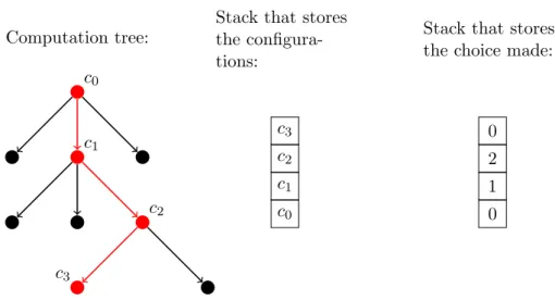
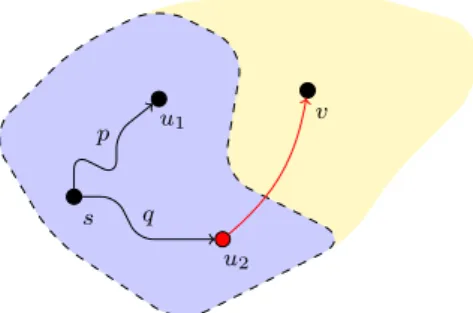
We directly start with the second inclusion. The result makes use of a space-economic way to store a stack for a depth-first search in a tree. An illustration of the idea used in the proof can be seen in Figure 4.1.

Theorem 4.12. Let t:N→N be a function, then we have:

NTIME(t(n))⊆DSPACE(t(n)).

Proof. Let M be a non-deterministic Turing machine that is t(n)-time- bounded. To discover an accepting configuration of M deterministically, we do a depth-first search on the computation tree ofM. We construct the tree on-the-fly and accept if an accepting configuration is encountered.

The depth of the tree is t(n) and each configuration needs t(n) space.

Hence, a simple solution that stores a stack of configurations needsO(t(n)²) space. But there is a more efficient way:

There exists akthat only depends onM such that every non-deterministic choice in the computation tree of M is at most k-ary. Since we only have to reconstruct the path from the initial configuration to the configuration currently visited, we only need to store the choices we made on this path.

(31)

Computation tree:

c0

c1

c2

c₃

Stack that stores the configurations:

c3

c₂ c1

c₀

Stack that stores the choice made:

0 2 1 0

Figure 4.1: To perform a depth-first search in the computation tree of the Turing machine, we need to store a stack. Instead of saving a configuration in each stack frame, we only store the choices that we made on a path through the tree. This is enough to reconstruct the path and it is a significant saving of space.

There are at mostkchoices, so that in each stack frame we only need constant space. Hence, we can reconstruct the current configuration inO(t(n)) space: Start with the initial configurationc0(x) and then simulateM using the stack to resolve choices.

Theorem 4.13. Let s:N→Nbe a function so that s(n)≥logn. Then we have the following inclusion:

NSPACE(s(n))⊆DTIME(2^O(s(n))).

Proof. Let us first assume that s(n) is space constructible. We use this assumption to determine the set of all configurations that use space at most s(n). To enumerate the configurations, we encode them as strings:

• The states are given numbers and we write them down in unary.

• To separate the components of a configuration we use a fresh symbol (i.e. #).

The strings encoding each configuration have length at most d·s(n), for some constantd.

For the actual enumeration, we first mark d ·s(n) cells. This can be done since s(n) is space constructible. We use these cells as reference to enumerate all strings of length d·s(n) in lexicographic order. For each of

(32)

the enumerated strings, we check whether it is a configuration. Altogether, the enumeration can be done in 2^O(s(n)) time.

On the resulting set of configurations, we do a reachability check. We may do a least fixed point and mark the reachable configurations (An alternative would be to enumerate the edges and to do a graph traversal).

To this end, we repeatedly scan all configurations and mark them if they are reachable via the transition function δ. One scan needs 2Ô(s(n)) time and we have to do at most 2Ô(s(n)) scans. Hence, the reachability check needs 2Ô(s(n))·2Ô(s(n))= 2Ô(s(n)) time.

To get rid of the assumption of space constructibility, we do the above procedure for a fixed space bounds= 0,1,2, . . .. If we encounter a configuration that needs more space than s, we set s := s+ 1. We eventually hit s(n) in which case no configuration needs more space. The time requirement is then:

s(n)

X

s=0

d^s= d^s(n)+1−1

d−1 ∈2^O(s(n)).

(33)

Chapter 5

Savitch’s Theorem

Goal: The most important question in Theoretical Computer Science is the question whether P = NP. A similar question arises for the classes DPSPACE and NPSPACE. The relation between them was solved rather early by Walter Savitch. In this chapter, we will prove Savitch’s Theorem:

Theorem 5.1 (Savitch, 1970). Let s:N→Nbe a function so that s(n)≥ logn. Then we have:

NSPACE(s(n))⊆DSPACE(s(n)²).

In particular, NPSPACE=DPSPACE and typically referred to as PSPACE.

For proving the theorem, we generalize acceptance of a Turing machine to the problem PATH in a directed graph, the configuration graph. A proper definition is given below:

Definition 5.2. The following problem is called PATH:

Given: Configurationsc₁, c₂, and a time boundt.

Question: Can we get from c1 toc2 in at mostt steps.

Our goal is to solvePATHdeterministically ins(n)² space. Since the configuration graph has size 2^O(s(n)), we want to solve reachability in a directed graph withn nodes deterministically in (logn)² space.

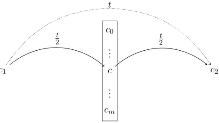
The main idea to achieve this space bound is to search for an intermediate configurationcand recursively check

• whetherc₁ can get toc in ₂^t steps and

• whetherc can get toc₂ in ₂^t steps.

If we reuse the space for each of the checks, we obtain a significant saving of space. Figure 5.1 provides an illustration of the procedure.

(34)

c₁

c₀ ... c ... c_m

c₂

t 2

t

Figure 5.1: In order to check whetherc1 can reachc2 in at most tsteps, we look for an intermediate configurationc so thatc1 can reachcin at most ^t₂ steps and ccan reachc₂ in at most ₂^t steps. This is applied recursively.

The algorithm needs space for storing a stack. Each stack frame has to hold c₁, c₂, the current intermediate configuration c and the countert, stored in binary. Since t ∈ 2^O(s(n)), by Lemma 4.7, such a frame can be stored in O(s(n)). The depth of the recursion is logt. Hence, the stack needs the following space:

O(s(n))

| {z }

stack height

· O(s(n))

| {z }

stack frame

=O(s(n)²)

Proof. We may assume that s(n) is space constructible. Otherwise we can apply the enumeration trick from Theorem 4.13. Since the given NTM M is s(n)-space bounded, we also know that it is c^s(n)-time bounded by Lemma 4.7. In Theorem 4.13, we also discussed how configurations ofM can be encoded as strings of lengthd·s(n) over an alphabet Γ.

Letα, β ∈Γ^d·s(n). We write

α−→^≤k β

if α and β represent configurations of M and α can go to β in at most k steps without exceeding the space bounds(n). The deterministic algorithm will now check if

c_init−→^≤k c_acc,

where cinit and cacc denote the initial and the accepting configurations of M. We can assume c_acc to be unique: by deleting the tape content, moving left, and only then accept.

The function to checkα −→^≤k β is described by the deterministic algorithm, Algorithm 1. It is clear that we have:

sav(α, β, k) = true iffα−→^≤k β

(35)

Algorithm 1 sav(α, β, k)

1: if k= 0 then

2: return (α=β)

3: end if

4: if k= 1 then

5: return (α→β)

6: end if

7: if k >1then

8: for all γ ∈Γ^d·s(n) enumerated in lexicographical orderdo

9: if γ is a configuration then

10: bool a_{lef t}:=sav(α, γ,d^k₂e)

11: bool a_right:=sav(γ, β,b^k₂c)

12: if a_{lef t}∧a_right then

13: return true

14: end if

15: end if

16: end for

17: return false

18: end if

For the space requirement, consider the following: the depth of the recursion is log(c^s(n)) = O(s(n)). Each stack frame contains α, β, γ and the value k stored in binary. This needs 3·d·s(n)+log(c^s(n)) =O(s(n)) space. Together, we obtain the space bound: O(s(n)²). We can get rid of the constant using tape compression, see Lemma 3.8.

(36)

Chapter 6

Space and Time Hierarchies

Goal: In this chapter, we show that higher space and time bounds lead to more powerful Turing machines. We will useUniversal Turing machines to separate space and time classes by strict inclusions.

Recall 6.1 (The proof technique diagonalization). Show the existence of a languageLwith certain properties, i.e. space requirements, that cannot be decided by a Turing machine taken from a given set{M₁, M₂, . . .}. To this end, start with some languageL1, decided byM1 and having the property.

Fori > 1, change the language Li−1 toLi so that Li still has the property but none of M₁, . . . , Mi−1 decides L_i. The limit of this construction is the languageL, we are looking for.

For the following Lemma, we provide two different proofs. The first one makes use of an uncountable set, the second proof uses the diagonalization technique described above.

Lemma 6.2. There are undecidable languages.

First proof. The set of languages over{0,1} isP({0,1}^∗) and therefore uncountable. The set of Turing machines is countable. Hence, there are languages which cannot be decided by Turing machines.

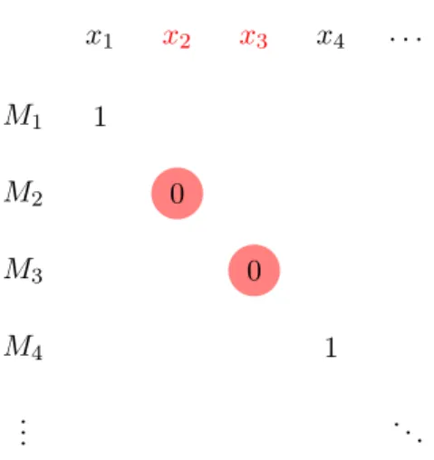
Second proof. Let x1, x2, . . . be an enumeration of all binary strings and M₁, M₂, . . . an enumeration of all Turing machines over {0,1}. Define the language:

L={xi∈ {0,1}^∗|Mi(xi) = 0}

An illustration of the languageL can be found in Figure 6.1.

Now assume that there exists a Turing machine M that decides L. Then there is an i∈N such that M = Mi. Now consider the string xi ∈ {0,1}.

then there are two cases:

(37)

M1

M₂ M3

M₄ ...

x₁ x₂ x₃ x₄ . . . 1

0 0

1 . ..

Figure 6.1: The stringsx2 and x3 are not accepted by the Turing machines M₂, respectively M₃. Hence, these two elements are in the language L.

Sincex₁ and x₄ are accepted byM₁, respectivelyM₄, these two strings are not inL.

• IfM(xi) = 1 then Mi(xi) = 1. So, xi ∈/ L butM(xi) = 1, which is a contradiction.

• If M(x_i) = 0, then M_i(x_i) = 0. So, x_i ∈L, but M(x_i) = 0, which is again a contradiction.

Hence, L cannot be decided by a Turing machine. This finishes the proof.

6.1 Universal Turing Machine

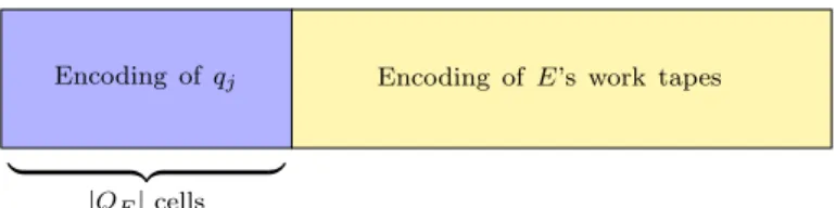
Goal 6.3. To make use of diagonalization, we have to encode and simulate Turing machines. For the encoding, we will use aG¨odel numbering of Turing machines, for the simulation we will make use of auniversal Turing machine.

The size of the encoding that we use will be a constant since we fix our Turing machine. So there is no need to be space efficient and indeed, we will see that we encode TMs unary. In contrast to this, the universal Turing machine has to beefficient. It has to obey space and time bounds.

Let us start with the encoding of deterministic Turing machines into{0,1}^∗. Definition 6.4. LetM = (Q,Σ,Γ,$, , δ, q_init, q_acc, q_rej) be ak-tape deterministic Turing machine. Moreover, let

Q={q_init

|{z}

=q1

, q_acc

|{z}

=q2

, q_rej

|{z}

=q3

, . . . , q_|Q|}

Complexity Theory