Design of a multi-modal transportation system to support the urban agglomeration process

Design of a multi-modal transportation system to support the urban agglomeration process

Allister Loder

^a,∗

, Andrew Schreiber

^c

, Thomas F. Rutherford

^b

, Kay W. Axhausen

^a

a

Institute for Transport Planning and Systems, ETH Z¨ urich, Switzerland

b

Department of Agricultural and Applied Economics, University of Wisconsin-Madison, USA

c

National Center for Environmental Economics, EPA, USA

Abstract

Improvements to urban transportation systems are designed to reduce travel times, but can also facilitate additional productivity gains through agglomeration. These systems, however, are complex, making it difficult to identify and quantify the mechanisms that improve eco- nomic productivity. In this paper we propose a quantitative urban spatial equilibrium model with simple urban structure that incorporates endogenous agglomeration and multi-modal congestion to study the transportation policy effects of investment and pricing on economic productivity. The model features a novel traffic flow modelling tool called the multi-modal macroscopic fundamental diagram (MFD). This modelling tool allows us to account for ef- fects of network topology and multi-modal traffic operations in the macroscopic modelling of congestion. We use the model to show how policy decisions regarding investment in the public transport system and the pricing of two modes of transport (cars and buses) influence economic sorting and thus urban productivity in the greater Z¨ urich metropolitan area.

Keywords: congestion, MFD, agglomeration, public transport, equilibrium model

1. Introduction

People use transportation systems to spread ideas and goods by travelling for work and leisure. Improvements to the system reduce time spent in traffic and allow this scarce resource to be used more productively for other activities (Glaeser, 1999; Levinson, 2012).

The movement of people to activities, however, is not evenly distributed across space, but rather concentrated in specific locations as we see globally in the existence of cities. Such

∗

Corresponding author Phone: +41 /(0)44-633-6258

E-mail address: allister.loder@ivt.baug.ethz.ch

concentrations result from agglomeration and dispersion forces and their understanding has implications for urban policy making and economic development as appropriate land-use policies provide opportunities to increase inhabitants’ welfare (Ahlfeldt et al., 2015; Allen et al., 2015; Allen and Arkolakis, 2019). A remaining challenge for adequate policy making is to understand the physics of multi-modal congestion in the formation of agglomeration and dispersion forces as all large cities rely not only on cars, but also on public transport services and other modes.

Dating back to Marshall (1920), a large literature analysed how agglomeration externalities are generated through, e.g., labour market pooling, input sharing and knowledge spillovers;

see Duranton and Puga (2004) and Rosenthal and Strange (2004) for thorough reviews on the sources of agglomeration economies. Another part of the literature analysed its importance in economic development (e.g., Fujita et al., 2001; Fujita and Thisse, 2013; Bettencourt, 2013).

We contribute with this paper to the agglomeration literature that is particularly analyzing the relationship between economic activity and transport infrastructure or investment (e.g., Venables, 2007; Baum-Snow, 2007; Duranton and Turner, 2012; Donaldson and Hornbeck, 2016; Donaldson, 2018). The presence of a likely positive relationship implies that the transportation system not only provides mobility, but also that appropriate policies can support the agglomeration process and economic growth (Banister and Berechman, 2000, 2001).

¹

Transportation system policies can be considered from at least three design dimensions: in- frastructure investment, operations management and pricing. Modern cities usually support several transport modes (e.g., cars and buses) with varying costs and benefits between them.

An optimal system design balances these factors according to some primary objective, which brings up many questions relevant to policy: Should we invest in roads or public transport?

Should we increase car costs or increase public transport costs? These questions have been raised and answered many times already from a traffic perspective (e.g., Smeed, 1968; Yang and Bell, 1998; Anas and Lindsey, 2011; Tabuchi, 1993) and can have important consequences for economic productivity. So far, the link between these questions to agglomeration has only been established independently for each mode (e.g., Venables, 2007; Zhang and Kockelman, 2016), but not systematically whilst accounting for multi-modal interactions. This paper aims to close that gap.

Historically, cities have addressed these three dimensions (infrastructure, operations man- agement and pricing) to limit congestion and to promote economic development. Perhaps the most recognizable step taken was infrastructure investment into freeway systems, which increased total employment in city centres as well as productivity. However, such investment measures had considerable feedback effects, inducing decentralized housing decisions which increased the risk of congestion and may have negatively affected economic development (As-

1

This relationship then also factors into the question of optimal city size (e.g., Mills and de Ferranti,

1971; Henderson, 1974b; Arnott and Stiglitz, 1979; Tsekeris and Geroliminis, 2013).

chauer, 1989; Fernald, 1999; Baum-Snow, 2007; Hymel, 2009; Baum-Snow, 2010; Duranton and Turner, 2012; Holl, 2016; Baum-Snow et al., 2017). At a national scale, such investments can contribute to agglomeration benefits between cities through specialization (e.g., Silicon Valley) (Ellison and Glaeser, 1997, 1999; Venables, 2017). Investment in collective trans- portation modes (bus, tram, subway) is also seen as congestion relief (e.g., Yang et al., 2018;

Anderson, 2014; Beaudoin et al., 2015; Adler and van Ommeren, 2016), which, like invest- ment in roads, can lead to productivity gains (Graham, 2007a; Chatman and Noland, 2014), but can also have varying impacts on decentralization in cities depending on the extent of the network (Gonzalez-Navarro and Turner, 2018; Roth et al., 2012).

Operational features of the transport network such as signal settings and bus operations have not been explicitly linked to the agglomeration process, but have been shown to be important in traffic optimization. For example, there has been work on quantifying the efficiency implications of signal operations (e.g., Webster, 1958; Haddad and Geroliminis, 2012), bus priority (e.g., Guler and Menendez, 2014), bus lane allocation (e.g. Zhang et al., 2018; Zheng et al., 2017; Zheng and Geroliminis, 2013), and bus scheduling (Ceder and Wilson, 1986; Guihaire and Hao, 2008). The implications of pricing on congestion have also been a topic of concern in the literature. Road pricing has long been identified as a measure to decrease congestion (Pigou, 1920; Vickrey, 1969; Henderson, 1974a; de Palma and Lindsey, 2011), but so far, only a few cities have implemented such a system, e.g., London and Singapore (Prud’homme and Bocarejo, 2005; Leape, 2006; Anas and Lindsey, 2011).

Regarding shared modal choices, researchers argue that the price of public transport should be subsidized by the amount that it enhances welfare (Parry and Small, 2009; Small and Verhoef, 2007).

Not only has agglomeration been well understood and studied (e.g., Duranton and Puga, 2004; Rosenthal and Strange, 2001, 2004; Ciccone, 2002; Melo et al., 2009, 2017; Redding and Sturm, 2008; Ahlfeldt et al., 2015), but also the interaction between congestion and agglom- eration (e.g., Solow, 1972; Anas and Kim, 1996; Wheaton, 1998; Tabuchi, 1998; Anas and Xu, 1999; Wheaton, 2004; Arnott, 2007; Brinkman, 2016; Zhang and Kockelman, 2016; Graham, 2007b). However, as Chatman and Noland (2011) summarized “There is little discussion of public transport.” So far, accounting for physical multi-modal interactions in congestion or the operational features of public transport in economic models has been a rather complex and difficult task, as it usually requires extensive amounts of data and separate microscopic simulations. However, advances in research on the multi-modal macroscopic fundamental diagram (MFD) (Daganzo, 2007; Daganzo and Geroliminis, 2008; Geroliminis and Daganzo, 2008; Geroliminis et al., 2014; Loder et al., 2017, 2019b,a) provide the first opportunity to account for physical multi-modal interactions simultaneously within economic models with- out iterative model linking or simplistic assumptions. The MFD is an empirical framework that treats urban road networks as a system or a factory that produces trips, and where the system’s internal function explicitly accounts for network topology and traffic operations, e.g., signals and buses.

In this paper, we contribute to the literature with a quantitative urban spatial equilibrium

model with simple urban structure that incorporates agglomeration following Venables (2007) and the multi-modal MFD framework to describe endogenously multi-modal congestion and the effects of transport policies on congestion and productivity. In this model of a closed economy without external trade and urban growth, commuters choose where to live and work, their portfolio of mobility tools (car and/or bus season ticket) and their preferred mode of transport (car or bus). We use a measure of accessibility to economic mass based on Hansen (1959) as the link between changes in the transportation system and productivity. The model simultaneously solves for an economic and traffic equilibrium following exogenous changes in the prices for mobility tools or the stock of public infrastructure. Here, we illustrate the model’s applicability for the greater Z¨ urich metropolitan area, where we investigate the effects of changes to the attractiveness of the public transport system by varying ticket and car costs. We find that improvements to economic output and wages in Z¨ urich are realized by increasing the costs for cars and not by changing public transport pricing, while improvements also result from bus frequency improvements and more dedicated bus lanes.

This paper is organized as follows: section 2 introduces the model with its economic, traffic and sorting sub-models. In section 3 we summarize the model calibration. Section 4 presents four simulation scenarios of the effects of system design changes on urban productivity. We conclude the paper in section 5.

2. Model

The integrated model combines a spatially disaggregated economic equilibrium model of housing and labour markets with a transport equilibrium model of an urban network that includes mode (car and public transport for season ticket holders) and route choice.

²

In this integrated model we divide the city into several zones which can be thought of as neigh- bourhoods, whereby we use the terms “zones” and “nodes” interchangeably. The model is calibrated to reflect reference morning and evening commute times, as we want to investigate the effects of agglomeration on wages and productivity. All travellers in the network move from their home location to their work location. We denote the home location by subscript i and the work location by subscript j. All zones that a representative traveller must pass through from i to j are denoted by subscript k. Further, as real cities usually have a sub- stantial number of inbound commuters from the hinterland, we account for this by adding zones around the city without economic activity, i.e., without workplaces, which are strictly residential areas with a fixed population.

The economic model is composed of profit-maximizing, zone-specific aggregate production sectors all producing a homogeneous good, and utility-maximizing representative agents, de- nominated by where they live and work. This component of the model follows the Walrasian- Arrow-Debreu paradigm and is expressed in Harberger units. Representative agents (RA

_ij

)

2

An early iteration of this type of model is found in Schreiber et al. (2016).

Index Description i,j,k Zone identifier

m Mode identifier with values b for bus and c for car r Route identifier

t Mobility tool portfolio: just car, c; just season ticket, s; all tools, a

Table 1: Model sets

living in zone i provide labour to productive activities in zone j. Agents must choose where to live and work based on wages, housing prices and commuting times. Agents also choose their mobility tool portfolio t based on exogenous price levels. They further choose commut- ing modes and routes based on travel times that are endogenously computed in the transport equilibrium model. Following traditional urban economic models, a representative absentee landlord LL owns the capital and housing stocks in all zones and accrues rental payments from production sectors and households (Fujita and Thisse, 2013). The methodology used for representing agglomeration effects due to concentration in the workforce follows Venables (2007) with a gravity-based accessibility index. Empirical evidence for this link’s validity was provided by Axhausen et al. (2015).

The problem is formulated as a single mixed complementarity problem (MCP) implemented in the MPSGE (Mathematical Programming System for General Equilibrium) framework in GAMS (General Algebraic Modeling System). We first introduce the key ideas of MCP in the next subsection and subsequently discuss the economic sub-model, the transport sub-model and the sorting conditions.

In Table 1 we list all sets used in the notation of variables and parameters. Table 2 lists all model variables, and Table 3 lists all model parameters. Benchmark or reference values are represented by an overline.

2.1. Mixed complementarity problems

Complementarity problems are closely related to variational inequality (VI) problems (Nagur- ney, 1993) with the key difference that complementarity problems are only defined on the nonnegative orthant R

ⁿ+

. Consider x ∈ R

ⁿ

as a decision variable vector. Let h (x) : R

ⁿ+

→ R

ⁿ

then be a vector of continuous functions. The complementarity problem is to find a vector

¯

x ∈ R

ⁿ+

such that

h (¯ x)

^T

x ¯ = 0 (1)

h (¯ x)

^T

≥ 0 (2)

In Eq. (1), the constraint has to be either zero or the associated variable. This makes complementarity a feature rather than a requirement of the model. In Eq. (3) we use the

⊥ symbol to indicate the complementarity condition between the constraint and associated variable:

h (¯ x)

^T

≥ 0 ⊥ x ¯ ≥ 0 (3)

Mixed complementarity problems are formulated with both inequalities and equalities. Equa- tions with free complementary variables are not constrained to the nonnegative orthant.

2.2. Economic model

In this integrated model we consider a macroscopic perspective of a city with several separate zones for people to live and work. The model requires standard general equilibrium assump- tions (firms maximize their profits and households maximize their utility) while accounting for agglomeration effects on wages and productivity.

The economic sub-model assumes perfect competition and is characterized through three types of conditions: (i) activities (households and firms must make zero profits); (ii) supply must be greater than or equal to demand; and (iii) incomes must balance with expenditures.

In the following, we introduce each set of equations in that order.

2.2.1. Zero-profit condition

We denote Π

^Y_j

as the unit profit function for production in zone j (Y

_j

) and Π

^U_ij

as the unit profit function for the utility of living in i and working in j (U

_ij

). Using Shepard’s Lemma, input coefficients are calculated by differentiating the associated unit profit function with respect to input and output prices. Activity levels are the complementarity variables associated with zero-profit conditions. If costs exceed revenues, then the level of the activity must be zero.

In the production sector, a macro-output good is produced in each zone j according to Eq.

(4). Unit revenue is characterized by the homogeneous price P that is set to the numeraire.

The unit cost function assumes Cobb-Douglas technologies, combining labour in zone j (with the wage rate W

_j

), capital (at the rental rate R

_j

) and a specific factor (with the price P SF

_j

) to account for differences in production technologies and processes across the zones.

We calculate the benchmark level of zone-specific factors as the difference between each zone’s

gross product and the value added from labour and capital expenditures. The exponents in

the cost function in Eq. (4) denote the value shares for each production factor in a particular

zone j.

−Π

^Y_j

= −P + W

_j

W

_j

θ^l_j

R

_j

R

_j

θ_j^k

P SF

_j

P SF

_j

θ_j^s

≥ 0 ⊥ Y

_j

≥ 0 (4) In the household sector, the utility U

_ij

for the representative agent RA

_ij

living in zone i and working in zone j is composed of demand for leisure (with the price P LS

_ij

), the macro good at price P and demand for housing in zone i at price P H

_i

. We define utilities as given by Eq. (5) with a nested constant elasticity of substitution (CES) form. At the top level, demand splits between leisure and other goods combined in the composite good CG using Cobb-Douglas preferences.

−Π

^U_ij

= −P U

_ij

+

P LS

_ij

P LS

θ^ls

CG

^1−θ_i ^ls

≥ 0 ⊥ U

_ij

≥ 0 (5) In the nested layer, CG

i

combines the demand for the macro good and housing as given by Eq. (6). Preferences for the composite good follow an exogenously set elasticity of substitution, σ

^c

. The aggregate price of a unit of utility is represented as P U

_ij

.

CG

_i

=

θ

^c

P

^1−σc

+ (1 − θ

^c

) P H

_i

P H

1−σ^c

1/1−σ^c

(6) We assume in the benchmark that reference prices do not vary across agents choosing dif- ferent residence and work zones, implying identical preferences. We capture idiosyncratic preferences by solving the model for reference prices consistent with observed sorting be- haviours.

2.2.2. Market-clearing conditions

Market-clearing conditions are needed for each endogenous price in the model. First, the market-clearing condition for the homogeneous macro good is given by Eq. (7). As the good is not zone-specific, the total supply is the sum of all zones’ supply. The total demand for the macro good is the sum of the demand by the absentee landlord LL, who demands only the macro good, and the demand by each representative agent RA

_ij

.

X

j

∂Π

^Y_j

∂P ≥ LL P + X

ij

∂ Π

^U_ij

∂P ⊥ P ≥ 0 (7)

Second, the market-clearing condition for the labour market as given by Eq. (8) includes

the representation of agglomeration effects with the productivity index X

_j

. Thus, we scale

the labour force in j by the productivity index that represents productivity gains from increased worker density in a particular location. The effective wage therefore changes for the representative agent to W

_j

X

_j

.

X

i

N LW

_ij

X

_j

≥ ∂Π

^Y_j

∂W

_j

⊥ W

_j

≥ 0 (8)

Third, we assume that the capital stock in j , K

_j

, is fixed to a zone. Then the market-clearing condition for capital becomes Eq. (9).

K

_j

≥ ∂ Π

^Y_j

∂R

_j

⊥ R

_j

≥ 0 (9)

Fourth, similar to the case of capital, we further assume that specific factors SF

_j

are also immobile across zones and thus fixed. Then the market-clearing condition for the specific factor becomes Eq. (10):

SF

_j

≥ ∂ Π

^Y_j

∂P SF

j

⊥ P SF

_j

≥ 0 (10) Fifth, again similar to the cases of capital and the specific factors, we assume a fixed housing stock in each zone H

_i

. With this, the market-clearing condition for the housing market becomes Eq. (11):

H

_i

≥ X

j

∂Π

^U_ij

∂P H

_i

⊥ P H

_i

≥ 0 (11)

Sixth, the market-clearing conditions require a definition of leisure. We define total leisure N LS

_ij

as given by Eq. (12). The total supply of leisure N LS

_ij

depends on the sorting of representative agents N

_ijmr

. We assume that all agents have a total of 3 hours in the morning and in the evening that can either be used for leisure or for commuting, with travel time T

_ijmr

between i and j . Consequently, agents with longer commutes have less time for leisure (i.e., a lower N LS

_ij

).

N LS

_ij

= 2 X

mr

N

_ijmr

(3 − T

_ijmr

) (12)

The market-clearing condition for leisure is then given by Eq. (13), where we implicitly

assume that the value of leisure is not the same as the wage rate:

N LS

_ij

≥ ∂Π

^U_ij

∂P LS

_ij

⊥ P LS

_ij

≥ 0 (13) Last, the market-clearing condition for utility is given by Eq. (14):

∂Π

^U_ij

∂P U

_ij

≥ RA

_ij

P U

_ij

⊥ P U

ij

≥ 0 (14)

2.2.3. Income balance

For representative agents RA

_ij

, income consists of the wage income net of productivity gains and the value of their time. The expenditures of representative agents for mobility tools are the total flow of agents along m and r multiplied by the average price between origin and destination for a single traveller obtained with price Π

_ijt

for mobility tool portfolio t and its share of ownership Q

_ijt

. The income balance for representative agents thus becomes Eq.

(15).

RA

ij

= W

j

N LW

ij

X

j

+ P LS

ij

N LS

ij

− X

mr

N

ijmr

! X

t

Π

ijt

Q

ijt

!

(15)

We define Q

ijt

and Π

ijt

in Eq. (29) and Eq. (30) respectively. This analysis does not differentiate between different price or cost components and subsume all taxes, fares etc.

under the term costs.

Second, the absentee landlord, LL, is assumed to own all the capital, housing and specific factor stocks. Thus, the income balance becomes as given by Eq. (16). We assume that the revenue from mobility tools and mode use feeds into an external budget.

LL = X

j

R

_j

K

_j

+ P SF

_j

SF

_j

+ X

i

P H

_i

H

_i

(16)

2.3. Transport model

Both the congestion effects that factor into the sorting behaviour of agents and the agglom-

eration effects are obtained from the multi-modal or three dimensional (3D) macroscopic

fundamental diagram (MFD) (Geroliminis et al., 2014; Loder et al., 2019b). The MFD

describes a well-defined relationship between the number of vehicles in a region (or neigh-

bourhood) and the average space mean speed for an urban road network. The shape of this

relationship results from network topology, signal settings and route choices (Daganzo and

Geroliminis, 2008; Geroliminis and Daganzo, 2008). Trip times are determined by how many vehicles take the same path. The model can be perceived as a reservoir or bathtub model in which drivers of vehicles flowing in want to exit as soon as possible (Daganzo, 2007). The 3D-MFD is a straightforward extension of the unimodal MFD that distinguishes between two types of vehicles (cars and buses) and explicitly accounts for the interaction between both modes of transport.

Accordingly, we can use the MFD to obtain the travel time for a known trip length, and in case of the 3D-MFD, we can obtain travel times for each mode in each network while accounting for the interaction effects between the two modes. Mathematically, we describe the 3D-MFD in zone k with a functional form for the 3D-MFD proposed by Loder et al.

(2019b). We can then obtain speeds from the 3D-MFD for each mode using the functions proposed by Loder et al. (2019b). Notably, changes to the underlying 3D-MFD parameters from Table 3 alter the shape of the function. We can thus capture changes to the functional form due to investment and network configuration changes as well as their effects on speeds and network performance.

In the integrated model, commuters choose mode m and macro route r for their commute.

Macro routes need not be matched to the road network, as the reservoir model requires only the route distance within the network d

_ijmr

to obtain the travel times T

_ijmr

between i and j using mode m and route r (Yildirimoglu and Geroliminis, 2014; Yildirimoglu et al., 2015).

Based on the parameters in Table 3, we then define the 3D-MFD for each zone k and obtain for each mode m the speed function V

_km

as given by Eq. (17). Speed is a function of each region’s joint vehicle accumulation A

_km

, 3D-MFD

_km

(A

_km

).

V

_km

= 3D-MFD

_km

(A

_k,c

, A

_k,b

) (17)

We obtain the accumulation of cars in each sub-network A

_km

with Eq. (18) by summing up all commuting flows N

_ijmr

, through the respective sub-network, weighted by the fraction θ

_ijk,c,r

of the route through that sub-network.

A

k,c

= X

ijr

θ

ijk,c,r

N

ij,c,r

(18)

We consider that the accumulation of buses A

_k,b

results from the design of the bus network, following work by Daganzo (2010), as given by Eq. (19). Here we consider that α

_k

is a fixed feature of each zone and that z

_k

is a multiplier that indicates how many bus lines overlap on average.

A

k,b

= z

k

2B

_k

h

_k

3α

_k

− α

²_k

1 + α

²_k

/v

com,bus

(19)

The total travel time along a route r using mode m through several regions from i to j is then obtained with Eq. (20) as the sum of the travel time in each sub-network.

T

_ijmr

= X

k

θ

^d_ijkmr

d

_ijmr

V

_km

(20)

The actual path costs or generalized travel costs along route r using mode m, C

_ijmr

, combine the travel time T

_ijmr

with the shadow prices for mobility tool capacity constraints for cars CC

_i

(see Eq. (25)) and for season tickets CT

_i

(see Eq. (26)), and include additional waiting time for the bus network DY

_i

when buses are full (see Eq. (27)). Further, for bus travellers the C

_ijmr

also contain half the starting zone’s headway (public transport frequency) to account for waiting times as well as an amenity factor AF

_ijmr

that accounts for all other factors in mode choice. In the case of Z¨ urich, AF

_ijmr

can capture Z¨ urich’s strict parking policy, which features high prices and low supply and accordingly increases the generalized cost for cars.

The AF

_ijmr

is estimated in the calibration of the model.

C

_ij,c,r

= T

_ij,c,r

+ CC

_i

C

_ij,b,r

= T

_ij,b,r

+ CT

_i

+ DY

_i

+ h

_i

2 + AF

_ijmr

(21)

We adopt a stochastic user equilibrium with a scale parameter µ

^R

that ensures that com- muters choose routes and modes with the lowest perceived path costs rather than those with the actual lowest path costs. The formulation in Eq. (3) is adopted from Chen (1999) and further describes a logit-based choice of mode and route.

P C

_ijmr

= C

_ijmr

+ 1

µ

^R

log (N

_ijmr

) (22)

We consider the equilibrium conditions in the network by simply following the first Wardrop principle in MCP formulation (Wardrop, 1952; Nagurney, 1993). Routes r and m are only chosen, i.e., N

_ijmr

> 0 if the perceived path costs are equal to the minimum perceived path costs M C

ij

between i and j. If the perceived path costs exceed the minimum costs, the route is not chosen, i.e., N

_ijmr

= 0, which is captured in the complementarity condition.

P C

ijmr

− M C

ij

≥ 0 ⊥ N

ijmr

≥ 0 (23)

We further have to ensure that the entire demand between i and j, N LW

_ij

, is distributed

across all available routes and modes as given by Eq. (24). The minimum perceived path

costs M C

_ij

are complementary to this condition.

N LW

_ij

− X

mr

N

_ijmr

= 0 ⊥ M C

_ij

≥ 0 (24)

Last, we need to define capacity constraints for mobility tool ownership, as only the number of commuters who own a particular mobility tool can use the respective mode. In other words, the number of car commuters living in i cannot be greater than the number of available cars in i, as given by Eq. (25). The same holds for the number of season ticket owners, as formulated in Eq. (26). In both equations, Q

_ijt

denotes the shares of each mobility tool portfolio between i and j and N LW

_ij

denotes the total demand between i and j. The shadow price of this capacity constraint is CC

_i

for cars and CT

_i

for season tickets, which are nonzero once the inequality no longer holds.

X

j

(Q

_ij,c

+ Q

_ij,a

) N LW

_ij

− X

jr

N

_ij,c,r

≥ 0 ⊥ CC

_i

≥ 0 (25)

X

j

(Q

_ij,s

+ Q

_ij,a

) N LW

_ij

− X

jr

N

_ij,b,r

≥ 0 ⊥ CT

_i

≥ 0 (26)

The bus passenger capacity constraint is given by Eq. (27). Here we define for each sub- network k a passenger capacity P XC

k

that cannot be exceeded. If capacity is reached, bus users will experience an additional delay as given by the shadow price of this constraint, DY

_k

.

P XC

_k

− X

ijr

θ

_ijk,b,r^d

N

_ij,b,r

≥ 0 ⊥ DY

_k

≥ 0 (27)

We link the passenger capacity P XC

_k

to the accumulation of buses in each region according to Eq. (28). Note that overline variables denote benchmark values.

P XC

_k

= P XC

_k

A

_k,b

A

_k,b

(28)

We obtain the shares of mobility tool portfolio Q

_ijt

with a two stage logit-based choice,

where Q

_ijt

changes with the prices of the chosen portfolio Π

_ijt

. Travellers choose among

three options: just a car, just a season-ticket, or both. This set of options is a simplification

of choices typically available in Switzerland (e.g., Loder and Axhausen, 2018). Note that

for readability we omit the set indices ij for Q and Π in the following two equations. The

alternative specific constant (ASC) is the calibrated market share Q

_ijt

and the utility of each

alternative only changes relative to the calibration prices. Scale parameter µ

^M

captures the

price elasticity of mobility tool ownership. In Eq. (29), the first stage determines the shares of having all or both mobility tools (car and season ticket), while the second stage determines the shares between car and season ticket owners along those not having all mobility tools.

Note that in a logit model the shares always add up to one.

Q

_a

= Q

_a

exp Π

_a

/Π

_a

− 1 /µ

^M

Q

_a

exp Π

_a

/Π

_a

− 1

/µ

^M

+ 1 − Q

_a

Q

_c

= (1 − Q

_a

) Q

_c

exp Π

_c

/Π

_c

− 1

/µ

^M

Q

_c

exp Π

c

/Π

c

− 1

/µ

^M

+ Q

_s

exp Π

s

/Π

s

− 1 /µ

^M

Q

_s

= (1 − Q

_a

) Q

_c

exp Π

c

/Π

c

− 1 /µ

^M

Q

_c

exp Π

_c

/Π

_c

− 1

/µ

^M

+ Q

_s

exp Π

_s

/Π

_s

− 1 /µ

^M

(29)

The Π

_ijt

is calculated as given by Eq. (30), where F

_ijtm

gives the fraction of using mode m with mobility tool set t and ˜ d

_ij

is the average trip distance across all route and mode alternatives.

Π

_ijt

= π

_t^fix

+ X

m

π

^var_tm

F

_ijtm

d ˜

_ij

(30)

The F

_ijtm

is defined according to Eq. (31). I

_tm

is an indicator function that equals one if t = s & m = b or t = c & m = c, and equals zero otherwise. This implies that when having just a car or a season ticket, only the respective mode can be used, i.e. F

_ijtm

≡ 1.

Only when having all mobility tools, F

_ijtm

can be different from zero and is simply the number of mode m travellers of all travellers for each origin-destination pair having both mobility tools.

F

ijtm

=





 P

r

N

_ijmr

− N LW

_ij

P

t⁰

I

_t⁰_m

Q

_ijt⁰

Q

ijt

N LW

ij

, if t = a

I

_tm

, otherwise

(31)

2.4. Agglomeration effects

Agglomeration benefits are allowed to accrue from concentrating the workforce. Productiv-

ity in zone j increases if nearby areas employ more people. Put differently, productivity is

a decreasing function of distance between zones due to a decrease in the ability to engage

in knowledge spillovers, labour market pooling, etc. We capture the agglomeration effects

following Venables (2007) by using an agglomeration index X

_j

for each node j , which in-

creases as the employment density and accessibility to other workplaces ACC

_j

around zone

j increase. Though we assume perfect competition in production, X

_j

represents external

economies of scale.

We define the agglomeration index X

_j

as given by Eq. (32). In the benchmark equilibrium, X

_j

equals unity. The reference level of employment density in zone j is denoted by ACC

_j

. The parameters µ

^A

and β quantify the impact of accessibility to employment (i.e., economic mass) on productivity. Figuratively speaking, µ

^A

determines the slope of the relationship while β simply scales changes in economic mass to productivity.

X

_j

= 1 + β

ACC

_j^µA

− ACC

^µ

A

j

(32) We define the employment density and accessibility to workplaces around j as ACC

_j

accord- ing to Eq. (33).

ACC

_j

= X

i

LD

_i

M C

_ij

(33)

Eq. (33) provides a measure of economic mass in zone j with effective labour demand LD

_j

that combines the productivity gains represented by X

_j

multiplied by the total labour force at j , which is given by Eq. (34).

LD

_j

= X

i

N

_ij

X

_j

(34)

2.5. Sorting

The representative agents sort across residential and work locations following a two-step, logit-based assignment. In our two-step logit formulation we first have to compute a utility index for living at node i as given by Eq. (35). The constraint requires that if the utility from living in i and working in j , denoted as U

_ij

, changes relative to its benchmark u

_ij

, then U L

_i

can fluctuate to enforce that probability’s sum to one. Here θ

_ij^u

describes the share of all residents living in zone i and working in j . For example, if the utility levels across all people living in i but working elsewhere in the city increase, then the utility index also increases.

However, if the utility increases for some work locations but decreases for others, the relative difference determines how the utility index changes. Further, µ

^L

reflects an elasticity of housing location choice.

X

j

θ

_ij^u

exp 1

µ

^L

U

_ij

u

_ij

U

_i^L

− 1

= 1 (35)

The initial number of commuters choosing to live in i follows from Eq. (36). Changes

in utility as a result of system changes scale the benchmark number of people living in a

particular zone N L

_i

.

N L

_i

= N L

_i

exp (U

_i^L

− 1)/µ

^L

P

j

θ

^li_j

exp (U

_j^L

− 1)/µ

^L

(36)

The number of travellers living at i and working at j, denoted as N LW

ij

, follows from Eq.

(37). Here θ

_ij^u

N L

_i

represents the total number of residents of i working in zone j. Changes in the utility from living in i and working in j and in the living utility index U L

_i

scale the benchmark total following a working locational choice elasticity µ

^W

.

N LW

_ij

= N L

_i

θ

_ij^u









exp

1 µ^W

Uij

uijU_i^L

− 1

P

j⁰

θ

_ij^u0

exp

1 µ^W

U_ij0

u_ij0U_i^L

− 1









(37)

Variable type Symbol Description

Economic Y

_i

Production at node i

U

_ij

Utility realized living at i and working at j P Macro output price

W

_i

Wage rate in zone i

R

_i

Rental rate for capital in zone i P SF

_j

Price of specific factor in zone i P H

_i

Housing price in zone i

P LS

_ij

Shadow value of leisure for living in i and working in j P U

_ij

Unit price of utility for living in i and working in j LL Absentee landlord

RA

_ij

Representative agent living at i and working in j LD

j

Labour demand at node j

X

_j

Productivity index at node j

N X

_ij

Effective level of labour net of productivity gains N LS

ij

Total leisure travelling from i to j

ACC

_j

Accessibility index at node j

Transport T

_ijmr

Total travel times from commuting from i to j C

_ijmr

Total path cost from i to j

P C

_ijmr

Total perceived path cost from i to j V

_km

Speed of mode m in zone k

A

km

Accumulation of vehicles of mode m in zone k M C

_ij

Minimum perceived path costs between i and j

DY

_i

Shadow price of the bus passenger capacity constraint CT

i

Shadow price of the season ticket ownership constraint CC

_i

Shadow price of the car ownership constraint

Q

_ijt

Shares of mobility tool ownership between i and j Sorting U L

i

Utility from living at node i

N L

_i

Number of people living in i

N LW

_ij

Number of people living in i and working in j N

ijmr

N LW

ij

using mode m and route r

Table 2: Model variables

Parameter type Symbol Description

Economic θ

_i^l

Value share of labour in zone i θ

_i^k

Value share of capital in zone i

θ

_i^s

Value share of the specific factor in zone i θ

^ls

Value share of leisure

θ

^c

Value share of consumption

θ

_ij^u

Proportion of total residents at i working in j θ

_i^li

Proportion of total residents living at i

σ

^c

Elasticity of substitution in demand for the composite good K

_i

Reference level of capital stock in zone i

SF

_i

Reference level of specific factor stock in zone i H

i

Reference level of housing stock in zone i

u

_ij

Reference utility level for living in i and working in j β Productivity parameter measuring changes in productivity µ

^A

Parameter measuring impact of worker mass on productivity θ

_ij^u

Proportion of total residents at i working in j

θ

_i^li

Proportion of total residents living at i µ

^L

Elasticity of housing location choice µ

^W

Elasticity of work location choice

µ

^A

Impact of economic mass on productivity.

β Scaling of impact of economic mass on output.

Transport L

k

Infrastructure length network B

_k

Length of bus network

ϕ

_k

Share of dedicated bus lanes h

k

Headway of buses

z

_k

Bus line overlapping factor α

_k

Bus network design

AF

_ijmr

Amenity factor of mode m using route r d

_ijmr

Macro route distance

θ

_ijkmr^d

Share of route distance in zone k d

_ij

Average route length from i to j

µ

^R

Scale parameter of route and mode choice µ

^M

Price elasticity of mobility tool ownership P XC

_k

Public transport capacity in k

Π

_ijt

Total cost of mobility tool ownership for portfolio t between i and j

π

_t^fix

Fixed cost of mobility tool for mode m π

_tm^var

Variable cost of mobility tool for mode m

Table 3: Model parameters

3. Data and calibration

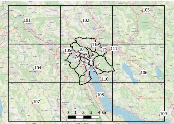
In this section we discuss data requirements and our calibration procedure for the integrated model. We first determine the spatial extent of the analysis. For the sake of simplicity, the economic activity zones and traffic zones are defined to be congruent. (However, the model can be applied to an arbitrary level of zoning.) This decision produces a trade-off between an optimal configuration of data for the transport sub-model and data availability in the economic model component. Whereas 3D-MFDs are well defined for homogeneous sub-networks with a surface area of a few square kilometres and a connected road network, we require a sufficient level of spatial specificity for economic information to capture variation in activity across the city. In this analysis, we follow the administrative and statistical zones within the city limits of Z¨ urich. The twelve zones of the city are called Kreise, and they are designated by number in ascending order from one to twelve. Kreis 1 and parts of Kreis 4 and Kreis 5 constitute the central business district. For inbound commuter zones where we do not want to analyse economic activity, we use a 3-by-3 grid. In general, the zoning outside of the economic activity area is arbitrarily constructed, but captures commuting from all cardinal directions. Figure 1 shows the zoning used for this analysis, with the city of Z¨ urich located in the middle of the map. Its boundaries are not aligned to the grid. In each zone we define a node from which the agents are assumed to start or end their trips.

Economic activity is described for zones 1 to 12 of the city of Z¨ urich. Inbound commuters from zones 101 to 111 (from the top left to the lower right) therefore cannot live and work in the same location. This kind of zoning and aggregation is, of course, a simplification of reality, but extending the model to comprise several nodes within a zone or many-to-one mapping of smaller statistical zones to 3D-MFD zones would be straightforward.

3.1. Economic data

The economic data used in the model was largely obtained from the city’s statistical offices.

Table 4 lists descriptive statistics and their sources. We match all data from a comparable

time period to provide consistency, limiting any outside exogenous variation. We proxy for

regional output levels (Y

_j

) by using a combination of regional gross product data, which

was disaggregated based on employment levels in each Kreis, and Kreis-level employment

and commercial property rental data. The number of employed workers was collected from

a national employment and workplace survey in 2008. Wages were obtained from a nation-

wide transportation survey conducted in 2015 by the Swiss Federal Statistical Office and

Swiss Federal Office for Spatial Development (2017). To calculate relevant wage levels, all

full-time employed respondents working in Z¨ urich were selected. As only household income

was reported in the survey, the reported household income is divided by the square root of

household members older than 18 years. Hourly wages are calculated by dividing monthly

Figure 1: Greater Z¨ urich region and applied zoning. The map is oriented to the north.

income by 160 working hours.

³

The value of the regional capital stock is composed of the value of commercial floor space and a specific factor. The specific factor is the unobservable component of the regional gross product, or rather, the difference between gross product levels and observed labour costs and commercial rent. In other words, we distinguish between the observable capital stock component labelled as capital generally, and the unobservable component labelled as a specific factor. The capital rental rate, i.e., the rent for commercial floor space, is available from a private company survey. Regional housing stock levels and prices are characterized by residential floor space and average rent. The average rent is a weighted average over all rented flats featuring 1 to 5 rooms.

The economic data present a relatively intuitive reference point. Many people work in Kreis 1, which features high wages and a limited housing stock, and live further from the city centre, primarily north or along the coast of the lake. Notably, there is limited variation in the housing rental prices which is consistent with the high cost of living in Z¨ urich.

3.2. Transport data

We require information on where commuters live and work (N LW

_ij

), the observed mode shares as well as the mobility tool portfolio choices of commuters. A commuter matrix for

3

Note that given our characterization of the labour market in Z¨ urich, the average Kreis-level labour value

share of production is 0.8.

KreisOutput(Y)1EmploymentWages(W)2Capitalstk.(K)3Officerent(R)4Housingstk.(H)3Housingprice(PH)3 (MilCHF/day)(Mil)(CHF/hr)(Milm2)(CHF/m2/day)(Milm2)(CHF/m2/day) 132.60.07145.51.21.40.31.1 220.10.03448.90.91.31.60.7 316.30.03443.70.90.72.10.7 412.30.03039.40.70.81.20.7 513.20.03543.11.30.90.70.6 65.90.01638.30.40.81.60.7 77.80.01939.40.51.02.20.7 89.10.02342.60.51.20.90.8 918.40.04039.61.30.72.20.6 104.10.01438.20.30.71.80.7 1115.00.04442.51.40.73.10.6 121.40.00533.80.10.61.10.6 1StatistischesJahrbuchderStadtZ¨urich2015;thecity’stotalGDPisdividedacrossKreiseaccordingtoemployment. 2SwissFederalStatisticalOfficeandSwissFederalOfficeforSpatialDevelopment(2017) 3StatistischesJahrbuchderStadtZ¨urich2014 4MarketsurveybyJLL(2015).

T able 4: Benc hmark v alues for the economic equilibrium.

Switzerland was previously made to generate a synthetic population for MATSim (a Multi- Agent Transportation Simulation) (B¨ osch et al., 2016). The essential information used in that commuter matrix had been collected by the Swiss government for the years 2010-2012 via a nation-wide census called a Strukturerhebung. The spatial resolution of the MATSim commuter matrix is higher than that of our applied zoning in Figure 1. We mapped the origins and destinations of that matrix to the zones used for this work and aggregated the data to line up with other data used in this analysis. Because the totals of the commuter matrix do not equal the workplace totals used in the Swiss national transport model for the city of Z¨ urich, we scaled the commuting matrix flows in N LW

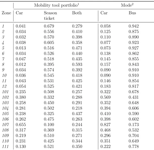
_ij

to match aggregate official employment statistics. Second, we used detailed trip diary information from the 2015 Swiss transportation survey to obtain information on mode shares (Swiss Federal Statistical Office and Swiss Federal Office for Spatial Development, 2017). We extract all commuting trips between the considered zones and calculated the share of car trips. Third, we used the aggregate information on mobility tool ownership in the present zoning to obtain benchmark values for the mobility tool portfolio choice Q

_ijt

. Table 5 summarizes the benchmark values for each zone in the analysis regarding mobility tool ownership and mode choice. People living within the Z¨ urich city limits (Kreise 1-12) largely have a season ticket and rarely rely on just a car for travel. This contrasts with individuals commuting from outside areas.

The data required for calibrating the 3D-MFD includes information on the topology of bus and road networks in the study regions as well as dynamic measurements (e.g., the flow of commuters) for both modes. Further, reference routes commuters follow from node i to j needed to be identified, particularly the trip distance using mode m on route r d

_ijmr

and the fraction of each route θ

_ijkmr

in each zone k.

For static information on the bus and road network we used data from OpenStreetMaps. For the road network length we focused on the main carriageways (trunk, primary, secondary and tertiary roads). For bus and tram networks we used all line networks within the greater Z¨ urich metropolitan area. Using these data, we calculated the total length of the network L as well as the bus network design α. Note that α can be greater than one in our case, as several lines overlap and/or run on dedicated infrastructure. However, this is not a problem, as we only need α to calculate changes in the bus services.

⁴

Dynamic measurements are available for all road-based public transport vehicles in Z¨ urich (see Loder et al. (2017) for further details). From this data set we calculate the free-flow speed of buses V

_0,b

, the average dwell time ∆, as well as the average accumulation of buses in the network during the morning rush hour A

_k,b

. The free-flow speed of cars V

_0,c

and the congested speed of cars V

_c

were obtained from data used by Amb¨ uhl et al. (2017). Table 6 lists all values and comments on their calculation.

For information on the reference macro routes, we queried the Google directions API and

4

We used the OpenStreetMaps API to download the data. Note that lines sometimes overlapped, in

which case we retrieved two line features.

requested directions from each zone’s centroid to all other zones’ centroids using either public transit or driving (avoiding highways) with at least one alternative route during peak hours.

From the API’s responses we created trajectories and calculated the length of each route d

_ijmr

. We then spatially overlaid the trajectories with the zoning from Figure 1 to identify the fraction of each route in each zone k and store the information in the parameter θ

_ijkmr

. 3.3. Behavioural parameters

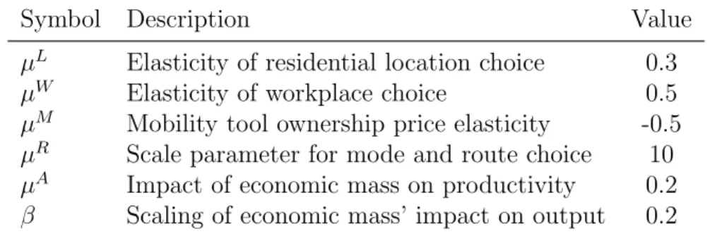
Table 7 summarizes the relevant behavioural parameters of the model. Given a yearly moving rate of roughly 10 % (van Nieuwkoop, 2014), we assume a rather inelastic choice of residential location and consequently set µ

^W

= 0.3. We consider that the labour market is slightly more elastic than the choice of residential location and thus set µ

^W

= 0.5. We oriented the value of the price elasticity of mobility tool ownership µ

^M

on long-term fuel price elasticity, which has been reported to be in the interval of [−0.5; −0.1] (Erath and Axhausen, 2010). Since we expect city residents to exhibit a higher willingness to substitute mobility tools, we set µ

^M

= −0.5. We set the scale parameter of the combined mode and route choice to µ

^R

= 10 to maintain deterministic aspects. Last, regarding the impact of economic mass on productivity, we follow the conservative values given by Venables (2007) for µ

^A

and β. However, to test the sensitivity of results with respect to the agglomeration parameters, we repeat the analysis with β = 0 and β = 0.4.

3.4. Calibration steps

To calibrate the transport equilibrium we use the parameters listed in Table 6 as references that we want to reproduce with our model. For this we use the amenity factor AF

ijmr

, the total network length L

_k

in each sub-region k, the public transport design α

_k

and the bus overlapping factor z

_k

. We use a three-step routine for the calculation of these parameters to reproduce the values from Table 6. The resulting values are listed in Table A.8 in the appendix.

In the first step, we fix speeds to the observed values from Table 6 and calculate the path

costs without an amenity factor, as given by Eq. (21). We then solve a nonlinear program for

each origin-destination-pair with AF

_ijmr

as a variable that minimizes the squared difference

between observed origin-destination mode shares and a logit choice of mode and route. As in

logit only differences matter, we set AF

_ij,b,r

= 0. In the second step, we calibrate the network

equilibrium by changing the total network length L

_k

in each zone. Arguably, infrastructure

use depends on traffic flows in which some streets might be empty while others experience

heavy congestion. Adopting L

_k

accounts for this. We solve the transport network equilibrium

again, but with AF

_ijmr

and speeds V

_km

as positive variables. We then iteratively change

the network length L

_k

, redefining the MFD speed function in Eq. (17) until the sum of the

squared differences between speeds from Table 6 and the equilibrium speeds are less than

0.001. In the third step, we solve a nonlinear program for each sub-region that uses α

_k

and

z

_k

as variables to minimize the squared difference between the observed number of buses from Table 6 and Eq. (19).

In order to calibrate the economic model component, we initially specify each representative

agent’s benchmark preferences to be the same and allow the model to adjust leisure prices

to account for differences in sorting behaviour. We also introduce a rationing quantity

instrument that adjusts the housing stock to match observable housing prices. Recalibrated

parameters are stored for use in the integrated model. When we integrate both parts of the

model, we validate the benchmark by verifying that the residuals at the zeroth iteration are

negligible. In other words that the observed reference values of the model variables (e.g., the

sorting of commuters, economic activities and the speeds) are reproduced by the model.

Mobility tool portfolio

¹

Mode

²

Zone Car Season

ticket

Both Car Bus

1 0.041 0.679 0.279 0.058 0.942

2 0.034 0.556 0.410 0.125 0.875

3 0.032 0.570 0.398 0.110 0.890

4 0.038 0.605 0.358 0.077 0.923

5 0.013 0.516 0.471 0.073 0.927

6 0.034 0.526 0.440 0.138 0.862

7 0.047 0.518 0.435 0.145 0.855

8 0.012 0.395 0.593 0.157 0.843

9 0.034 0.574 0.392 0.090 0.910

10 0.036 0.545 0.418 0.090 0.910

11 0.043 0.531 0.425 0.146 0.854

12 0.054 0.525 0.421 0.183 0.817

101 0.235 0.508 0.257 0.322 0.678

102 0.380 0.332 0.288 0.569 0.431

103 0.258 0.450 0.291 0.352 0.648

104 0.281 0.502 0.218 0.394 0.606

105 0.238 0.325 0.437 0.410 0.590

106 0.262 0.475 0.263 0.398 0.602

107 0.655 0.100 0.244 0.827 0.173

108 0.317 0.369 0.315 0.468 0.532

109 0.219 0.510 0.271 0.296 0.704

110 0.231 0.425 0.344 0.351 0.649

111 0.130 0.521 0.350 0.222 0.778

1

Calculated as the share of all people employed in each zone based on the 2015 Swiss transportation survey (Swiss Federal Statistical Office and Swiss Federal Office for Spatial Development, 2017), irrespective of their actual mode choices. Those without any mobility tool were assigned to the group of season ticket holders.

2

Calculated as the share of all outbound commuting trips from each zone according to the 2015 Swiss transportation survey.

Table 5: Benchmark shares of mobility tool ownership and mode choice.

Kreis V

0,c1

V

c2

V

0,b4

∆

6

h

3

A

b4

B

k5

(km h

-1

) (km h

-1

) (km h

-1

) (s) (min) (-) (lane-km) 1 31.2 9.7 16.5 27 6 141 26.9 2 37.9 13.1 25.3 26 6 89 34.7 3 34.4 13.0 22.7 22 6 116 39.4 4 31.8 10.16 21.3 29 6 64 14.5 5 36.3 11.6 23.1 18 6 41 15.9 6 36.5 13.3 22.9 20 6 72 30.1 7 36.0 15.0 22.3 32 6 65 28.1 8 36.9 18.1 22.3 17 6 38 18.8 9 36.0 14.7 25.1 26 6 118 47.4 10 38.1 15.8 26.2 18 6 116 34.1 11 36.8 13.7 24.5 26 6 145 43.9 12 36.9 13.3 27.5 23 6 37 23.2

1Estimatedaveragespeedforcarjourneysbetween05:30to06:00basedonTomTom’sspeedprofilesdata-baseasusedbyAmb¨uhletal.(2017). 2Estimatedaveragejourneyspeedsfortheweekdaymorningpeakfrom08:00to08:30basedonTomTom’sspeedprofilesdata-baseasusedby Amb¨uhletal.(2017). 3Providedbypublictimetableinformation. 4Estimatedbasedonatrajectorydatasetofallpublictransportlines.Estimatedasthemeanduringtheweekdaymorningpeakfrom08:00to 08:30. 5FollowingthedefinitiongivenbyDaganzo(2010).

T able 6: Benc hmark v alues for the transp ort net w ork and equilibrium.

Symbol Description Value µ

^L

Elasticity of residential location choice 0.3

µ

^W

Elasticity of workplace choice 0.5

µ

^M

Mobility tool ownership price elasticity -0.5 µ

^R

Scale parameter for mode and route choice 10 µ

^A

Impact of economic mass on productivity 0.2 β Scaling of economic mass’ impact on output 0.2

Table 7: Behavioural parameters

4. Simulations

We use the calibrated integrated model to study the effects of changes to the public transport system on urban productivity. We first simulate how frequency changes to public transport (measured as headway) affect output (section 4.1). Second, we quantify the effects on ag- glomeration of reallocating dedicated space to or away from buses (section 4.2). Finally, we study how the agglomeration process is influenced by season ticket pricing (section 4.3) and by variable car costs (section 4.4). To test the sensitivity of the model with respect to the impact of agglomeration and to see whether agglomeration is important to consider, we simulate the models with the agglomeration impact parameter β ∈ {0; 0.2; 0.4}.

Recall that changes in mobility tool ownership Q

_ijt

only result from exogenous price changes, as discussed in sections 4.3 and 4.4. However, they do not result from or respond to changes in network topology, as discussed in sections 4.1 and 4.2.

4.1. Public transport service frequency

Our first scenario describes the outcomes of changing headway, or the time between arriving public transport vehicles. We model this shock by altering h

i

on all zones i which imposes additional (or lessened) time costs for public transport. The prices of the mobility tools remain unchanged and therefore, given our construction of the model, the shares of mo- bility tool ownership Q

ijt

also remain unchanged. However, because a certain share of the population has access to both mobility tools, changing the headway influences their mode choices.

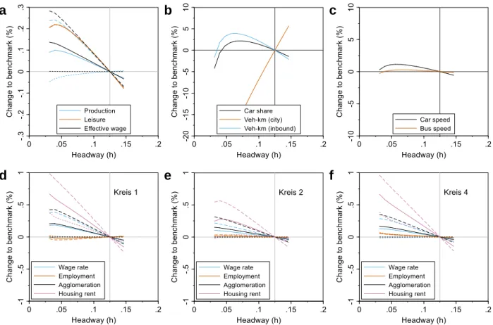
In Figure 2 we summarize the macroscopic effects observed from varying the headway from its benchmark value 0.125h in the interval from 0.03 to 0.15. Figures 2a-b show the changes for city totals, and Figure 2c shows the changes for the entire city averages. Figures 2d-f provide the results for zones (Kreise) 1,2, and 4. Figures 2a and 2d-f also provide the results for different impact levels of agglomeration as a sensitivity analysis, with a short dashed line corresponding to β = 0, a solid line corresponding to β = 0.2 and a long dashed line corresponding to β = 0.4. The figures in the following subsections are identically structured.

In Figure 2a we see that decreasing the headway increases total output and leisure and raises the effective wage for β > 0. In the case of β = 0, the effective wage changes only marginally due to changes in the labour markets. Better access by bus results in more commuters choosing workplaces in the central city zones, as wages there are higher.

Increasing the supply of workers decreases wages, consequently resulting in a decrease of output (see Eq. (8)).

⁵

Contrary to intuition, we find in Figure 2b that the modal split increases with decreasing headway, but this behaviour can be explained by differentiating the total vehicle kilometres by zone. City residents drive to work less with a decrease

5

Given our parameterization, increasing headway beyond 0.15h leads to a breakdown of the transportation

system, as the existing infrastructure is not able to accommodate all potential passengers.

a b c

d e f

Figure 2: Transportation system and economic market responses to changes in public transport service frequency. In panels a and d to f, the solid line corresponds to β = 0.2, while the short dashed line corresponds to β = 0 and the long dashed line corresponds to β = 0.4.

in headway, leaving more space on the streets which is then filled by inbound commuters who had previously used public transport. Because the inbound commuters’ trip distances are longer, the modal split increases. Figure 2c shows that improving the bus system’s headway improves the journey speeds of both modes, despite the effects observed in Figure 2b. Comparing spatial effects at the zonal level in Figures 2d-f shows that increasing bus frequencies shifts employment from Kreis 1 to the other Kreise. Increased accessibility to other zones increases the productivity of the workforce and results in higher wage levels.

Housing prices increase across zones given higher incomes and demands.

4.2. Dedicated public transport infrastructure

Our second simulation scenario proxies for changes to dedicated public transport infrastruc-

ture by altering the number of bus lanes available to commuters. Because we do not vary

the mobility tool prices there will be no change in Q

_ijt

. However, as in section 4.1, mode

choice and location choice effects can still be observed for the portion of the population with

access to both modes.

a b c

d e f

Figure 3: Transportation system and economic market responses to changes in the shares of dedicated public transport infrastructure. In panels a and d to f, the solid line corresponds to β = 0.2, while the short dashed line corresponds to β = 0 and the long dashed line corresponds to β = 0.4.

In Figure 3 we summarize the macroscopic effects observed when increasing or decreasing the

length of bus infrastructure by -50 to 50 % compared to the benchmark. We see in Figures

3a-c that more dedicated bus lanes increase economic output and leisure in the system

and raise the effective wages in the case of β > 0, while changes in the total wages again

remain small in the case of β = 0. Increasing the number of bus lanes increases bus speeds

throughout the system, leading to more time spent for leisure and increased productivity

through improved ease of access. These gains are obtained by shifting demand towards bus

transportation, that is, by improving the journey speeds of both modes. In Figures 3d-f

we report represenative spatial impacts. Reducing the number of bus lanes reduces access

to the city centre and reduces the attractiveness of working there. Because the elasticity of

residential location choice (µ

^L

) is relatively smaller than work choice elasticity, price impacts

are more pronounced for housing than for wages. However, the direction of impacts at the

zonal level is heterogeneous. For instance, employment increases with decreasing bus lanes

in the first and fourth zones, but decreases in zone 2. In the former case, more people are

willing to supply labour to these zones given longer commute times, which results in lower

wages. Wage changes are particularly pronounced with larger levels of β. While employment

0 .2 .4 .6 .8 1 Share (-)

0 2 4 6 8 10

Ticket cost (CHF/day)

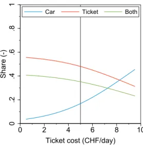
Car Ticket Both

Figure 4: Shares of mobility tool ownership as a function of season ticket costs

does increase, our measure of accessibility decreases in the formulation of the productivity index X

j

given increases in the perceived cost of travel between nodes. In contrast to Kreis 1, Kreis 4 shows increases in housing rent as a result of fewer bus lanes, indicating that more people are interested in moving there given the close proximity to zones with high wages.

The converse is reported for Kreis 2 (a largely residential zone stretching down the coast of the lake), given lessened demand for living further away from high-wage zones.

4.3. Public transport season ticket pricing

In addition to changes in infrastructure, changes in transportation pricing can influence commuting behaviour and economic sorting. In our third scenario, we vary the season ticket price from 0-10 CHF/day (around its benchmark value of 5 CHF/day). The exogenous price change leads to changes in the shares of mobility tool ownership Q

_ijt

, as shown in Figure 4.

Lower season ticket prices cause the share of car-only commuters to decrease and shares of season ticket holders and ownership of both mobility tools increase. Price changes lead to an uptake or drop in the ownership of a second mobility tool.

In Figure 5 we summarize the results of this scenario, showing network-wide effects in Figures

5a-c and spatial effects for Kreise 1, 2 and 4 in Figures 5d-f. Decreasing or increasing the

ticket price did not impact economic output at all, except for changing the agents’ income,

or the transportation system’s performance. This is explained by Figure 4, which shows

that many car drivers choose to hold a season ticket as a second mobility tool but do not

drop their car. Subsequently, this system change does not force them to change their travel

behaviour when making route and mode choices. Conversely, when the season ticket price

is increased, economic and transport performance decrease as seen in Figure 5a-c, leading

to an increase in car use (see Figure 5b) that consequently decreases both modes’ speeds,