Total Instructional Time Exposure and Student Achievement:
An Extreme Bounds Analysis Based on German State-Level Variation
Philipp Mandel Bernd Süssmuth
CES IFO W ORKING P APER N O . 3580
C
ATEGORY5: E
CONOMICS OFE
DUCATIONS
EPTEMBER2011
An electronic version of the paper may be downloaded
• from the SSRN website: www.SSRN.com
• from the RePEc website: www.RePEc.org
• from the CESifo website: Twww.CESifo-group.org/wpT
CESifo Working Paper No. 3580
Total Instructional Time Exposure and Student Achievement:
An Extreme Bounds Analysis Based on German State-Level Variation
Abstract
Using pooled data on instructional time and student performance by subject, our study finds evidence for the school inputs-student achievement relationship for German states. This finding is robust both to the inclusion of state fixed effects and in an extensive extreme bounds analysis. It stands in contrast to the majority of related studies. We argue that this is due to an error-in-variables problem and implied misinterpretation of existing studies that disregard the fact of learning being a cumulative process by relying on rather poor proxies for instructional time. Highschool ninth graders from the OECD Programme of International Student Assessment (PISA-E) tests’ bottom percentiles bene.t most from extra-instructional time measured in cumulated form from first up to ninth grade. Besides total instructional time exposure, we identify eight further social environment and institutional variables with robust impact on student performance. In contrast to instructional time hardly any of these factors can be affected by policy in the short run.
JEL-Code: I210, I280, L380.
Keywords: education production function, student performance, school resources.
Philipp Mandel
Institute for Empirical Research in Economics (IEW) / Econometrics
University of Leipzig Grimmaische Strasse 12 Germany – 04109 Leipzig mandel@wifa.uni-leipzig.de
Bernd Süssmuth
Institute for Empirical Research in Economics (IEW) / Econometrics
University of Leipzig Grimmaische Strasse 12 Germany – 04109 Leipzig suessmuth@wifa.uni-leipzig.de
We thank Carolin Amann, Fabian Feierabend, Constantin Tabor, Stephanie Najort, Marcus Strobel, Bastian Gawellek, and Alexander Mandel for excellent research assistance, particularly, in assembling the data. Thanks are also due to Marco Sunder for many helpful comments and suggestions.
1 Introduction
This paper is in the tradition of the seminal study by Card and Krueger (1992) in that it relies on cross-state variation in education inputs and institutions. There is a continuing debate on whether schooling resources have a bearing on student outcomes (Krueger 2003; Hanushek 2003, 2004, 2006a). Todd and Wolpin (2003) see econometric misspeci…cation and failure to account for major determinants of student achievement as the central problem in correctly identifying the relationship. Recently, a little studied input receives growing attention: In Coates (2003), Eren and Millimet (2007), Marcotte (2007), Marcotte and Hemelt (2008), and Lavy (2010) the focus is on instructional time by subject.
Our study is unique in using data of instructional time cumulated from all academic years leading up to the test date in each of the two subjects math and reading. We rely on cross-state variation in Germany, where 16 states share the same cultural and legal system but pursue di¤erent education policies (Schulte 2004). The fact that German states have responsibility for both primary and secondary education, makes our data particularly suited to analyze the impact cumulative instruction has on student achievements. As for the educational instruction–performance relationship, Marcotte (2007) and Marcotte and Hemelt (2008) are the only studies that focus on and consider the cumulative nature of instruction as determinant of student performance. They make use of intra-state school level and snowfall (unscheduled closings) data for students in grades 3, 5 and 8 in Maryland. Their approximation of a cumulated e¤ect is based on the hypothesis that the lower the grade, the less room exists for making up and the higher the relative weight of lost instruction. Therefore, the instructional time shortfall e¤ect decreases with grade. However, this cumulated e¤ect is of second order as only measures of total snowfall in the academic year of the test date (Marcotte 2007) or in the preceding 3 years (Marcotte and Hemelt 2008) are considered. Coates (2003) relying on district-level data for Illinois and considering uncumulated daily instruction in third grade classes, …nds that a 10 percent increase in mathematics instruction per week raises the average math score by about 0.4 percent. Similar small e¤ects are found for English instruction. Eren and Millimet (2007) analyze the joint e¤ect the daily number of class periods and the average class length (in minutes) has on cognitive test results of US public schools 10th graders (National Education Longitudinal Study of 1988). Only uncumulated 10th grade instructional conditions are considered. Their reform-type …nding is that changing the
system from one with 6 daily classes lasting 51 minutes to another one with seven 45-minutes classes increases test scores by 2 percent.
In sociology of education, sociolinguistics, and the neurosciences, a recent body of lit- erature is concerned with the structured processing of knowledge ascribing it to di¤erent modes of learning. An essential element of these modes is to conceptualize knowledge- building through cumulative learning. Accordingly, learning is found to be a cumulative process during which new knowledge is dependent and based on a precedingly acquired stock of knowledge; see, among others, Freebody et al. (2008), Maton (2009), and Yew et al. (2011). Yet, to the present, empirical work in the economics of education literature does not take these …ndings into account and relies on rather poor measures of instruc- tional time as independent variables. This is not to say that the relevance of current and past inputs and the de…ciencies of approaches abstracting from input histories is not recognized in the literature (Card and Krueger 1996, Todd and Wolpin 2003). It is simply and mostly due to data limitations not done. Typically, estimates are based on instructional time proxies such as students’self-reported hours of instruction per week as they relate to the respective test year. Todd and Wolpin (2003) refer to these measures as “contemporaneous inputs.” Given insights from sociology and neuro-sciences or, in general, from “multidisciplinary empirical literature studies”(Todd and Wolpin 2003, p.
F3), however, a cumulative measure such as cumulated instructional time (henceforth, CIT) from …rst grade to test year for each observed cohort is required. This becomes all the more obvious if we look at an arbitrarily chosen mathematics sample task from PISA (OECD 2009, p. 125) that reads as follows:
Mathematics Unit 27: A result of global warming is that the ice of some glaciers is melting. Twelve years after the ice disappears, tiny plants, called lichen, start to grow on the rocks. Each lichen grows approximately in the shape of a circle. The relationship between the diameter of this circle and the age of the lichen can be approximated with the formula:
d= 7:0 p
(t 12) for t 12;
where d represents the diameter of the lichen in millimetres, and t represents the number of years after the ice has disappeared.
In the two questions that followed students are asked to calculate (Q1) the diameter of the lichen, 16 years after the ice disappeared and (Q2) the number of years that the ice disappeared at a spot, where the diameter of some lichen is found to be 35
millimetres. Most obviously (Q1) and (Q2) can be answered based on knowledge on subtracting, multiplying, taking roots, and the technique of substitution or trial and error that students acquired over several years starting from the very …rst grade. These skills might have barely something to do with instruction in the ninth grade.
The vast majority of studies analyzing data from international student assessments like PISA or TIMSS (Third International Math and Science Study) only considers instruc- tional time at the relevant grade level as an explanatory for test performance. Usually, these “snap-shot”-type measures of instructional time are drawn either from students’
self-reporting or from test add-ons such as principals’questionnaires as, for example, in Baker et al. (2004), Lavy (2010), and Wössmann (2010). Given the serious error-in- variables problem contained in these measures, it does not come as a surprise that their impact on student test scores is mostly estimated as not statistically di¤erent from zero (as, for example, in Wössmann 2010). Besides studies that use snap-shot query-based measures, there are few studies that rely on the length of a school day and/or the length of a school year to proxy instructional time as input in an education production or more general Mincer-type framework (Dewey et al. 2000, Lee and Barro 2001, Pischke 2007).
Two exceptional studies that try to consider, at least, partially the cumulative nature of learning are Afonso and St. Aubyn (2006) and Moser and Angelone (2009). The …rst of these studies makes use of a variable “intended instruction time in public institutions in hours per year for the 12 to 14-year-olds” cumulated for the three years preceding the PISA 2003 tests for 25 di¤erent countries. Similarly, Moser and Angelone (2009) also partially accumulate instructional time in Swiss cantons from seventh to ninth grade to estimate its impact on PISA 2006 scores. Again, as expected given the rough approxi- mation of total instructional time for both studies there is no clear-cut evidence for the input–achievement relationship. Afonso and St. Aubyn (2006) …nd no signi…cant evi- dence. The evidence reported in Moser and Angelone (2009) is mixed and depends on the subject studied. A signi…cant positive association is found for instructional time and test scores in math.
Our study contributes along two lines to the literature. First, it addresses the outlined serious error-in-variables problem and implied shortcoming in empirical work on educa- tion inputs and outcomes measured by international student test scores by using data on total instructional time that students were exposed to from …rst to ninth (i.e. test date) grade by subject. Secondly, besides quantifying the actual impact of cumulative instructional time on PISA test scores, we address model uncertainty and robustness,
which are also issues that are widely ignored in the literature, by using extreme bound analysis (EBA) techniques for our estimates.
The rest of the paper is organized as follows. Section 2 outlines our data and used methods. Section 3 reports and discusses our …ndings. Finally, Section 4 concludes.
2 Data and methodology
2.1 Data
Data on student achievement are drawn from the national extension of the PISA studies in 2000, 2003, 2006 (PISA-E) and from the …rst so-called “Ländervergleich 2009,”that is, the follow-up study of PISA-E. PISA as well as the Ländervergleich test representative samples of 15-year-old students in math, science and reading literacy (in 2003 also in problem solving – in 2009, exclusively in reading and English). PISA-E used the same tests as the international PISA study. Apart from high schools, profound variation in the tracking and tracking systems among the remaining school types makes a comparison of student achievement across German states for these types of schools virtually impossible (Prenzel et al. 2008). Some of the remaining school types actually not even exist in each German state. This system heterogeneity is not an issue for high schools, on which we will focus in the following. The PISA-E test’s sample size is several times the one of the international tests comprising two overlapping samples of 15-year-olds and ninth graders. Each sample covers about 40,000 students made of state samples ranging from 1,600 to 5,000 students for the 16 German federal states. Since German con…dentiality requirements preclude the use of student-level data across states, one is restricted to use pooled state-level data.1 German states mean performance is measured on a standardized scale: Just like for any PISA and/or PISA-E participating OECD country, state or province, scores for each subject and year are centered to an OECD mean of 500 and a standard deviation of 100. All our regressions include dummy variables for year and test subject, respectively.
Our data on instructional time are compiled from the respective state by-laws, taking
1Pooling is a common practice in the literature. An example for pooling subjects is Eren and Millimet (2007). Pooling German states and merging in data on aggregate countries is done in Wössmann (2010). Coates (2003) also considers pooling three test years.
into account amendments of ordinances, correcting for festivities and celebrations, such as state-wide holidays and any changes over time in these regulations for the period of observation. We followed the respective PISA cohorts from …rst to ninth grade. First to fourth grade concerns elementary school, …fth to ninth grade concerns high school (re- ferred to as “Gymnasium”in German). For each of the 16 states, we construct an annual instructional time variable that is summed up to CIT. The data used in the construction of the variable come from several sources. The major part is drawn from administrative regulations, which can be found in o¢ cial ministerial and/or school administration docu- ments or in law and ordinance gazettes of the states. For some federal states, information on instructional time is given in special by-laws, so-called “Stundentafelverordnungen,”
as well as in regulations and mandates concerning training, examination and school rules such as the Bavarian “Volksschulordnung (VSO)”for elementary schools and the “Gym- nasialschulordnung (GSO)” for high schools. In case of doubt and missing data, we obtained the information from the respective ministry of education and cultural a¤airs.
Data on weighting schemes for a di¤erent intra-state distribution of teaching focus at the high school level (natural sciences, modern languages, math, etc.) is drawn from the respective statistical o¢ ce’s database.
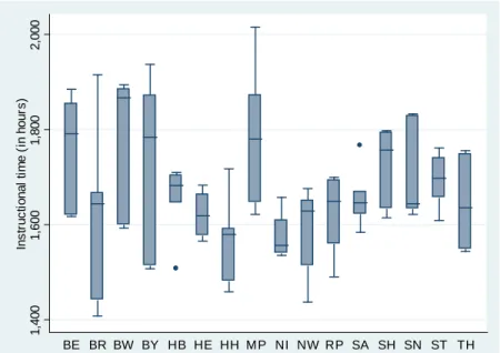
1,4001,6001,8002,000Instructional time (in hours)
BE BR BW BY HB HE HH M P NI NW RP SA SH SN ST TH
Figure 1. Math and reading CIT across states; PISA-E cohorts 2000/03/06/09
..
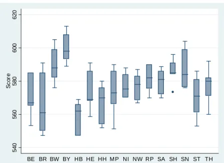
540560580600620Score
BE BR BW BY HB HE HH M P NI NW RP SA SH SN ST TH
Figure 2. Math and reading scores across states; PISA-E cohorts 2000/03/06/09
As reliable data on CIT, constructed according to the strategy sketched above, cannot be obtained for all test subjects, we restrict our analysis to math and reading. We should also be clear about the point that we do not consider unscheduled shortfall, homework, individual tutoring or private study taken before or after school. In sum, we comprise total curricular hours of the four test cohorts accumulated from year of primary school enrollment (1991/92, 1994/95, 1997/1998, 2000/2001) to test year (2000, 2003, 2006, 2009).
Pooling PISA-E and Ländervergleich data for math and reading over states, tested subjects (math, reading), and cohorts allows us to rely on a sample of 112 observations.2 As can be seen from Figure 1 and Figure 2,3 German states substantially di¤er both in test scores and cumulative instruction by subject. For the distributions shown in Figure 1 and Figure 2, there are two central sources of variation: changes over the considered
216 states, two subjects (math and reading) for three cohorts plus reading for the test cohort of 2009 amounts to16 2 3 + 16 = 112. It is frequently claimed that studies relying on data at the level of states or districts su¤er from an aggregation bias. Coates (2003) argues that the profession has not yet reached a consensus on whether such bias tends to produce spurious resource e¤ects or not. According to Wössmann (2010) aggregation bias is not an issue in the case of marginal e¤ects estimated using German state-level data.
3The following abbreviations are used: Berlin (BE), Brandenburg (BR), Baden-Wurttemberg (BW), Bavaria (BY), Bremen (HB), Hamburg (HH), Hesse (HE), Mecklenburg-West Pomerania (MP), Lower Saxony (NI), North Rhine-Westphalia (NW), Rhineland-Palatinate (RP), Saar- land (SA), Schleswig-Holstein (SH), Saxony (SN), Saxony-Anhalt (ST), Thuringia (TH).
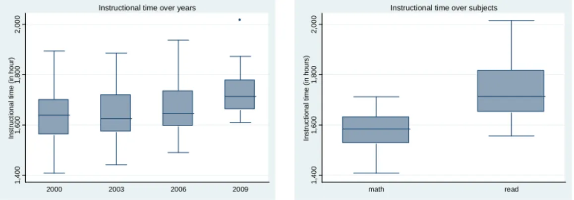
four waves and across the two subjects. Aggregated over states the distributions behind these two sources are shown in …rst and second schedule of Figure 3 and Figure 4, respectively. In order to check, whether it actually makes a di¤erence to consider CIT, we also compared the snap-shot (i.e. only test year concerning) “instruction time” variable used in Wössmann (2010, Table 2, p. 241, Table A.1, p. 266) for PISA-E 2003 and subject math4with our corresponding cumulative measure. The correlation is statistically insigni…cant at all conventional levels.
1,4001,6001,8002,000Instructional time (in hour)
2000 2003 2006 2009
Instructional time over years
1,4001,6001,8002,000Instructional time (in hours)
math read
Instructional time over subjects
Figure 3. CIT state-means distributions
540560580600620Score
2000 2003 2006 2009
PISA-Score over years
540560580600620Score
math read
PISA-Score over subjects
Figure 4. PISA-E test scores state-means distributions
2.2 Baseline estimates
To analyze the impact of CIT on students’test performance we rely on empirical models close to the ones common in the literature on education –or more speci…cally on cognitive achievement– production functions. See, among others, Hanushek (2002), Todd and
4The variable is constructed based on the PISA 2003 student questionnaire, in particular, on Q35b, Section F: Your mathematics classes. It reads as follows: “In the last full week you were in school, how many class periods did you spend in mathematics?” (OECD 2003, p. 24).
Wolpin (2003), Fuchs and Wössmann (2007), and Wössman (2003, 2010). Our baseline speci…cations are standard in the sense that we consider besides our central regressor (CIT) also sets of control variables that include measures of social environment and institutional features at the state level.
Table 1. Baseline estimates: PISA-E 2000, 2003, 2006
Without state …xed e¤ects With state …xed e¤ects
CIT 0.287
(0:096) 0.387
(0:034) 0.450
(0:016)
CIT2/1000 -0.075
(0:141) -0.112
(0:036) -0.126
(0:022)
Included set of controls
a) Economic x x x
b) Social x x
c) Educational x
N obs 96 96 96
Adj. R-Squ. (percent) 63.63 74.87 69.87
F statistics 19.47 10.43 8.87
0.325
(0:082) 0.385
(0:043) 0.380
(0:029)
-0.094
(0:084) -0.112
(0:044) -0.111
(0:030)
x x x
x x
x
96 96 96
72.19 72.77 78.61
11.28 9.75 9.73
Note: Estimates include subject and year dummies; , , denotes signi…cance at 10, 5, 1% level, respectively; p-values in parentheses; controls de…ned in text (and Appendix B).
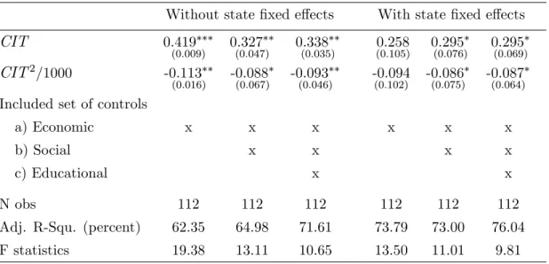
Table 2. Baseline estimates: PISA-E 2000, 2003, 2006, Ländervergleich 2009 Without state …xed e¤ects With state …xed e¤ects
CIT 0.419
(0:009) 0.327
(0:047) 0.338
(0:035)
CIT2/1000 -0.113
(0:016) -0.088
(0:067) -0.093
(0:046)
Included set of controls
a) Economic x x x
b) Social x x
c) Educational x
N obs 112 112 112
Adj. R-Squ. (percent) 62.35 64.98 71.61
F statistics 19.38 13.11 10.65
0.258
(0:105) 0.295
(0:076) 0.295
(0:069)
-0.094
(0:102) -0.086
(0:075) -0.087
(0:064)
x x x
x x
x
112 112 112
73.79 73.00 76.04 13.50 11.01 9.81 Note: Estimates include subject and year dummies; , , denotes signi…cance at 10, 5, 1% level, respectively; p-values in parentheses; controls de…ned in text (and Appendix B).
Concretely, in order to get a …rst assessment of the relationship, we estimate the following speci…cations
Sit = i+ f(CITit) +X3
g=1
Xkg
j=1 jXg;jit+"it; (1) whereSitdenotes test scores; indexiandtrefer to state and test period, respectively. We consider up to three sets of control variables, i.e.,Xg=1; :::; Xg=3, consisting ofk1 = 6 eco- nomic and political economy variables,k2 = 8social environment and socio-demographic variables, andk3 = 9education policy and institutional variables, respectively. The max- imum magnitude of conditioning variables amounts tok1+k2+k3 = 23. SetX1(economic controls) comprises conservative party shares of governments (Cons), per capita (p.c.) public indebtedness (Debt), p.c. disposable income (Disp), population densities (Dens), unemployment rates (Unemp), and p.c. GDP (GDP) …gures. Set X2 (social controls) consists of data on last and …rst cohorts experiencing secondary school fees (Fee, Fee2), female employment rates (Fem), shares of foreign population (For), segregation measured by the share of 15-year-olds attending high school (Seg), shares of students with migra- tion background (Mig), and dummies for East Germany (East) and city-state (City).
Finally, set X3 (education controls) considers secondary school years to …nal grade, i.e., either 8 or 9 years track (G9), average class sizes, student-teacher-ratios, instructional hours per teacher, and shares of part-time teachers in elementary school (CS1,ST1,HT1, PT1) and in secondary I (CS2, ST2, HT2, PT2), respectively. For further detail and sources of variables see Appendix B. A brief summary on how these variables might a¤ect student test scores is given in Appendix B.
Controlling for state …xed e¤ects i addresses the quali…cation of unobserved het- erogeneity across states. In particular, this concerns such unobservables as pedagogical quality, performance, and e¤ectiveness of teachers across states (Hanushek 2006b) as well as di¤erences in the quality of educating teachers. It also implies the quality of text books, instructional methods and materials, and the administration and organiza- tion of curricula. For all these dimensions each German state has its own choice and responsibility. As can be seen from the respective …rst three (common constant model) and last three columns of estimates shown in Table 1 and Table 2, a signi…cant positive e¤ect from CIT on test scores is robust to the inclusion of state …xed e¤ects. In fact, our estimates controlling for …xed e¤ects do not markedly di¤er from the ones obtained from regressions without considering state e¤ects. In speci…cation (1), we follow the most recent cross-country study by Lavy (2010) in allowing for concavity in the functional re-
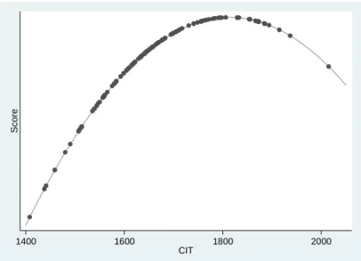
lationshipf( )between student performance and CIT. As can be seen from the estimates reported in Table 1 and Table 2, this more ‡exible speci…cation accords with the data, although less than ten percent of cases lie to the right of the implied upper turning point (Figure 5). For the remaining vast majority of data points in the scatter diagram, the relationship between CIT and test scores is close to linear. As Figure 5 is based on the estimates reported in the last three columns of Table 2, including state …xed e¤ects, it does not show ordinate values. Hence, we interpret it only qualitatively as lending sup- port to a weakly concave, nearly linear relationship. In the estimates reported in Table 1, we abstracted from using data from the Ländervergleich 2009, which in contrast to the preceding PISA-E tests did not test math skills of students. Again, the results are qualitatively not sensitive to the inclusion of the 2009 (reading) scores (Table 2). We leave all further quantitative interpretation of estimates for section 3, reporting results from our sensitivity analysis of the bearing CIT has on student test performance. In the following, we outline how we achieve robustness by addressing model uncertainty in an extreme bounds analysis framework.
Score
1400 1600 1800 2000
CIT
Figure 5. Relationship between CIT and test scores
2.3 Addressing model uncertainty: methodology
In order to address model uncertainty, we subject our empirical model to an extreme bounds analysis (EBA) as originally suggested by Leamer (1983, 1985) and Levine and Renelt (1992) and extended and modi…ed by Granger and Uhlig (1990) and Sala-i-Martin (1997). The use of EBA techniques is fairly popular in the empirics of economic growth
literature. However, its use is not limited to growth regressions. For recent applications in other contexts see Sturm et al. (2005) and Mossa (2009). Yet, we are not aware of an EBA application in the area of education production function estimates. In general, EBA does not include the use of state (or country) …xed e¤ects to take account of unobserved heterogeneity. In fact, in the present context the use of state …xed e¤ects implies that di¤erent average student PISA test scores between states are not explained but represented by dummy variables. Thus, all that can be explained by these regressions are reactions of test scores over time (see, in a similar context, Kirchgässner 2011, p. 17), which show a comparatively lower variation than the distribution of scores across states.
See the distributions shown in Figure 2 as opposed to the ones shown in the …rst diagram of Figure 4. Following this argumentation and adhering to the EBA practice in the literature, we abstract from the inclusion of state dummies as well as from nonlinear speci…cations. Both modi…cations have shown to be not critical for an assessment of the relationship between CIT and student test scores (section 2.2).
Hence, our general EBA speci…cation reads Sit= + CITit+Xn
j=1 jVjit+Xm
k=1 kZkit+ it; (2)
whereVj represents a set of important variables included in every regression. It contains a dummy for subject math as well as dummy variables identifying the respective year.
Zk is a set of three up to eleven out of 23 possible conditioning variables (section 2.2), where the minimum number of such conditioners (= 3) follows the suggestion in Levine and Renelt (1992). To identify di¤erences between the impact of CIT on average PISA-E test scores and of CIT on scores of top and bottom percentile students of each cohort, we also consider T opX% and BotX% as dependent variables. To check for robustness, the strategy is to consider all possibleM =n!=(k!(n k)!)regression models that can be estimated by taking combinations ofkout of the 23Z-variables, that is,1;771models for k = 3up to 1;352;078 models fork = 11. For this elaborated sensitivity analysis we also address for every single regression in the procedure possible problems of multicollinearity by dropping models with a variance in‡ation factor (VIF) for the exogenous at stake exceeding a value of four.5
As proposed by Levine and Renelt (1992), so-called “extreme bounds” of estimates
5A V IFj for some exogenous variable xj is de…ned asV IFj = 1=(1 R2j), where goodness- of-…t measureR2j refers to a regression ofxj on all other independent variables in the respective model. For zero collinearityV IFj takes on a value of one.
can be used to check whether a variable likeCITit in eq. (2) is fragile or robust. They are made of lower and upper bound. The former is de…ned as the lowest estimated value for
M minus two standard deviations, the latter as the highest estimated value for M plus two standard deviations. If lower and upper extreme bound for estimated coe¢ cients show the same sign, the explanatory variable at stake is said to be robustly related to the dependent variable.
A critical aspect of EBA-techniques in their original version proposed by Leamer (1983) and Levine and Renelt (1992) is that extreme bounds may be resultant from models that are unreasonable in terms of a corresponding relatively low R2 statistics.
A modi…ed EBA procedure addressing this problem is suggested by Granger and Uhlig (1990). Their idea is to consider only those M estimates stemming from models that reachR2 statistics corresponding to a certain percentage of the Rmax2 of all M estimated models, taking into account the goodness-of-…t R2min of the basic model (leaving out the control for conditioning variables, i.e., Xm
k=1 kZki). This approach is referred to as
“reasonable extreme bounds analysis”(REBA) in the literature. For model speci…cations with R2-values equal to or greater than
R2 = (1 )Rmax2 + R2min; (3) where 0< <1 and for small -values, we consider corresponding speci…cations as being
“reasonable” speci…cations as they are not too far o¤ from the “best” model –of the M considered ones–in terms of goodness-of-…t as measured by the adjusted R2.
Sala-i-Martin (1997) argues that a single regression for which the sign of the coe¢ cient changes or becomes insigni…cant su¢ ces according to original EBA or REBA standards that a variable is identi…ed to be non-robust. He assesses this procedure as a too hard to pass test for almost any variable at stake: “if the distribution of the parameter of interest has some positive and some negative support, then one is bound to …nd one regression for which the estimated coe¢ cient changes signs if enough regressions are run”(Sala-i-Martin 1997, p. 179). This insight led Sala-i-Martin to introduce a newly modi…ed approach by moving away from the extreme test and instead assigning some level of con…dence by looking at the entire distribution of the estimators of M. For each of the M estimated models the likelihood LM, the point estimates M, and the standard deviation M are calculated. They are used to construct the mean estimate of and the average variance
2 as a weighted average of M point estimates and estimated variances, respectively:
=XM
l=1!M M; 2 =XM
l=1!M 2M; (4)
where weights!M are proportional to the likelihoods of the M models according to
!M = LM XM
l=1LM
: (5)
Once the mean and the variance of the distribution of , assumed to be normal,6 are known, the cumulative distribution function (CDF) can be calculated using the standard normal distribution. The level of con…dence for the variable of interest is de…ned as the larger of the two areas under the probability density function (PDF) left and right from zero.7 In order to be as comprehensive as possible, we apply all three methods, that is, standard EBA, REBA, and EBA in the modi…ed version of Sala-i-Martin (1997), hence- forth SiM-EBA. Primarily this is done to check the robustness of the association between CIT and PISA scores, letting k vary between 3 and 11. Going beyond this primary sensitivity analysis, we also scrutinize the impact of the other 23 potential explanatories (see Appendix B for detail) on our measure of cognitive achievement Sit relying on the considered portfolio of EBA-techniques.
3 Results
3.1 Cumulative instructional time
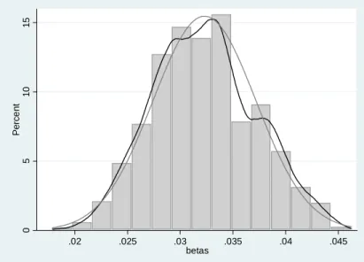
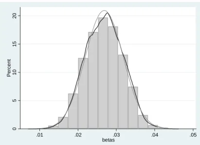
Results for all three EBA methods outlined above are reported for three di¤erent (max- imum) numbers of variables sampled into the conditioning set, i.e., for k = 3; k = 5, and k = 11, in Table A.3, Table A.4, and Table A.5 of Appendix A, respectively. In the interpretation of these …ndings, we will follow Sala-i-Martin and focus on the entire distribution (SiM-EBA) and only discuss results from the other two procedures if they deviate from the SiM-EBA based …nding. For all used dependent variables, CIT shows a positive signi…cant impact on scores that is robust if we consider di¤erent subperiods, even if we apply CDF(0) > 0:95 as more strict criterion of robustness. A …rst point to note is that variation in k does not qualitatively alter our results as can be seen from Table A.3 to A.5 in Appendix A. Figures 6 to 8 make the point by showing the respective
6The normality assumption is justi…ed on the grounds of the central limit theorem as can be seen from Figures 5 to 7.
7We follow Sala-i-Martin (1997) by referring to the larger of the two areas as “CDF(0)”
irrespective of whether the area lies actually above or below zero.
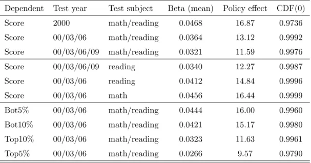
distribution of estimated coe¢ cients for di¤erent k (the black line drawn through the respective diagram shows the kernel density, while the grey line depicts the normal PDF as a reference case). The distributions virtually have the same mean, while the variance, of course, decreases with k and the number of estimated models M. CDF(0) remains above a value of 0.95 going from k = 11 to k = 3, that is, narrowing the number of variables contained in the conditioning set. This suggests for the sake of e¢ ciency, that is, for the sake of estimating rather 33,649 (k = 5) than 1.35 million (k = 11) models for di¤erent test waves or subsets of pooled waves (Table 3), to concentrate the further analysis on k = 5. Table 3 reports these results for all students’ scores as well as for the top-5% and top-10% and the bottom-5% and bottom-10% of students in terms of test scores. Since for Ländervergleich 2009 no score data by percentile is available our analysis for bottom-/top-end students is restricted to the PISA-E waves 2000, 2003, and 2006. For the overall test scores as dependent, we consider besides the total pool also a corresponding data set restricted to the year 2000 only and one that leaves out the Ländervergleich 2009, when math has not been tested. The year 2K test sub-sample captures the e¤ect of the …rst year in which the test was conducted. In this sense, it can be seen as relatively free from e¤ects induced by policies that the states started in the aftermath of the …rst test. This is due to the fact that results from the PISA-E 2000 tests were widely published and extensively discussed in the media and in political debates (Tillmannet al. 2008, Pütz 2008). As can be seen from Table 3, we also considered total and sub-set sample separately for math and reading sub-samples. The fourth column of Table 3 displays the unweighted mean of M for M = 33;649: Multiplying these …gures with an average of 360 (= 40 9) school weeks over the nine years from …rst grade to test date, we can calculate the approximate e¤ect of a policy corresponding to one additional hour of instructional time per week over the total learning period. It is shown in the
…fth column of Table 3. Finally, the last column in Table 3 reports CDF(0) values from applying the SiM-EBA method. As can be seen from the third line of results displayed in Table 3, the above described stylized policy e¤ect of CIT on scores amounts to siz- able 11.59 test-score points or roughly 12 percent of an international standard deviation.
Dropping the Ländervergleich 2009 data the e¤ect increases to more than 13 percent.
The largest average impact of a one hour per week increase policy is calculated, when one restricts the sample to the …rst year when German states ran the OECD PISA test for the …rst time, i.e. for PISA-E 2000. It amounts to nearly 17 percent of an inter- national standard deviation. For the sub-samples separating subjects, we …nd that the
e¤ect is particularly pronounced for math (>16 percent) but still sizable, that is, above 12 percent of an international standard deviation, for reading. Looking at upper and lower percentiles of test scores, we …nd that all students would bene…t from an increase in CIT. The CIT–score relationship is, however, more pronounced for the bottom-end students in terms of test scores, suggesting that those students would bene…t the most.
051015Percent
.02 .025 .03 .035 .04 .045
betas
Figure 6. Distribution of estimated betas for SiM EBA: k = 3, pool: 00/03/06/09, math/reading
M = 1;771 models, N = 112 observations
05101520Percent
.01 .02 .03 .04 .05
betas
Figure 7. Distribution of estimated betas for SiM EBA: k = 5, pool: 00/03/06/09, math/reading
M = 33;649 models, N = 112 observations
05101520Percent
.01 .02 .03 .04 .05
betas
Figure 8. Distribution of estimated betas for SiM EBA: k = 11, pool: 00/03/06/09, math/reading
M = 1;352;078 models, N = 112 observations
To get an impression of what 16 percent of an international standard deviation is actually to mean, consider the following experiment of thought: Under the assumption that the policy of increasing the instructional time by one additional hour per week over the total learning period has a similar impact on scores for other secondary school types as it has for high schools, we can calculate the consequences in the rankings, interpreting German states “as a microcosm for OECD countries” (Wössmann 2010). Take OECD PISA 2006, in which German students ranked 14th in math compared to the other OECD test participating countries; see Table A.7 in Appendix A. An increase by 16 percent of the standard deviation (normed to 100) of this test would correspond to running up six ranks up to rank 8. In contrast, cutting CIT down by one hour per week would correspond to a drop in the ranking down to rank 24. Similar e¤ects can be calculated for reading.
All results reported in Table 3 are robust in the sense of Sala-i-Martin (1997).8 CDF(0) values range between 0.9736 to 0.9999. As can be seen from detailed Tables A.3, A.4, and A.5 in Appendix A, virtually all values for lower and upper bounds show positive signs, con…rming the highly robust positive e¤ect of CIT on PISA test-scores.
8Re-running our estimates relying on a snap-shot measure like the ones discussed in the introduction and used, for example, by Wössmann (2010), throughout generates results that are not robust (“fragile”) in the sense of any conventional EBA-criterion (EBA, REBA, SiM- EBA). Results are available on request from the authors.
Table 3. Impact of CIT on PISA-E tets-scores: SiM-EBA (k = 5; Z = 23) Dependent Test year Test subject Beta (mean) Policy e¤ect CDF(0)
Score 2000 math/reading 0.0468 16.87 0.9736
Score 00/03/06 math/reading 0.0364 13.12 0.9992
Score 00/03/06/09 math/reading 0.0321 11.59 0.9976
Score 00/03/06/09 reading 0.0340 12.27 0.9987
Score 00/03/06 reading 0.0412 14.84 0.9996
Score 00/03/06 math 0.0456 16.44 0.9999
Bot5% 00/03/06 math/reading 0.0444 16.00 0.9960
Bot10% 00/03/06 math/reading 0.0421 15.17 0.9980
Top10% 00/03/06 math/reading 0.0323 11.63 0.9961
Top5% 00/03/06 math/reading 0.0266 9.57 0.9790
Note: Policy e¤ect is one additional hour of CIT per week over total learning period.
3.2 Other robust determinants of cognitive achievement
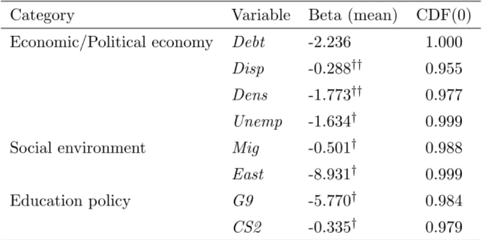
In order to analyze which of the remaining 23 available explanatories (see Appendix B for detail) have a robust impact on test scores, we rely on the same portfolio of EBA- techniques as for CIT in the preceding paragraphs. Table 4 below summarizes the results for this exercise reported in detail in Table A.6, for which we set k = 3 (M = 1;771)9 and consider the 00/03/06/09–math/reading pool withN = 112observations for each of theM estimated models. As central criterion of robustness we again apply the modi…ed SiM-EBA criterion, i.e. CDF(0) > 0.95.10
At the federal state level, public indebtedness (Debt), disposable income (Disp), pop- ulation density (Dens), and the unemployment rate (Unemp), each measured for the year corresponding to the respective PISA-E test-year, as well as a dummy for East German states (East) are found to be robustly and negatively associated with test scores accord- ing to the modi…ed SiM-EBA criterion. Drawn from the respective PISA cohort data, also the share of 15 years old students with migrational background (Mig) is identi…ed as
9As for CIT, results are qualitatively una¤ected by setting k= 5 (M = 33;649).
10Note, applying the less strict CDF(0) > 0.90 instead, as originally proposed in Sala-i- Martin (1997), also identi…es variables average class size in elementary schools (CS1), average instructional hours per teacher in elementary schools (HT1) and segregation (SEG) as robust determinants of student achievement.
robust negative correlate with scores. By this standard robust education policy variables are the number of secondary school years to exit exam (G9) and average class size in secondary I (CS2).
Table 4. Robust and weakly robust determinants of PISA-E test-scores besides CIT SiM-EBA (k = 3, Z = 23)
Category Variable Beta (mean) CDF(0)
Economic/Political economy Debt -2.236 1.000
Disp -0.288yy 0.955
Dens -1.773yy 0.977
Unemp -1.634y 0.999
Social environment Mig -0.501y 0.988
East -8.931y 0.999
Education policy G9 -5.770y 0.984
CS2 -0.335y 0.979
Note: ySiM-EBA, REBA: robust, standard EBA: fragile
yySiM-EBA: robust; standard EBA, REBA: fragile
The only variable that measures up to CIT with regard to meeting all robustness cri- teria of the considered portfolio of EBA-techniques is public indebtedness per inhabitant.
It proxies the cost e¤ectiveness of incumbent and former governments of the respective state. In terms of size, the estimated average coe¢ cient (<0) of the dummy for an East German state (East) stands out. This is, in particular, due to the poor performance of students from the East German state of Brandenburg (BR) as well as to the below national average achievement in terms of math and reading test scores of the two East German states Mecklenburg-West Pomerania (MP) and Saxony-Anhalt (ST); see Figure 2. It is also these states of the …ve East German ones that are known for their notori- ously unsound economic and demographic status characterized by a substantial number of movers to the Western states in the decades following German uni…cation. The average negative impact of the institutional grade con…guration variableG9 on test scores also is relatively sizable.11 The e¤ect is negative and amounts to about six percent of an inter- national standard deviation. It is straightforward to attribute this e¤ect to di¤erences in
11VariableG9 is a dummy that takes on a value of one if the number of secondary school years to …nal grade, that is, to Abitur, the German A-level equivalent, is nine as opposed to eight years. It is up to each state’s discretionary education policy to set this length. East German states traditionally practice an eight years system.
the density of curricula: Students might be comparatively more advanced in math and reading skills in a system, where the …nal exit exam takes place three rather than four years after the PISA test date. State-level population densities, unemployment rates, and shares of students with migration background show the expected sign (see Appendix B), though being less strongly associated with lower test scores in terms of size of estimated coe¢ cients. Another education policy variable that is robust according to the modi…ed SiM-EBA criterion is average class size in secondary I (CS2). A decrease ofCS2 by one student over the nine years from enrollment (…rst grade) to test year (ninth grade) is robustly associated, however, with only a minor increase of 0.335 points or 0.335 percent of an international standard deviation. In sum, the e¤ect of (education) policy variables is either most probably resultant from PISA tests being not adjusted to di¤erences in curricula or is quite small in size compared to the policy e¤ect of increasing CIT. The only counter-intuitive and weakest, in terms of size, e¤ect is the negative average coe¢ cient for disposable income.
A …nal caveat concerns the above interpretation of results reported in Table 4: Apart from public indebtedness per inhabitant and CIT all other 22 considered determinants of student achievement are either not robust or are fragile, at least, according to one criterion in the used portfolio of EBA-procedures. Hence, they have both some positive and some negative support (Table A.6).
4 Conclusion
Econometric misspeci…cation and failure to account for major determinants of student achievement represent the central problem in correctly identifying the school inputs–
student achievement relationship (Todd and Wolpin 2003). By relying on a portfolio of extreme bounds analysis techniques as well as a newly compiled cross-state dataset on cumulative instructional time from …rst grade to ninth (i.e., OECD PISA-test date) grade for German states, we addressed two fundamental shortcomings in the literature:
A serious error-in-variables problem due to using poor proxies of instructional time and the widely ignored issue of model uncertainty. We …nd that instructional time by sub- ject, measured in cumulative terms, is a highly robust determinant of student cognitive achievement. This …nding is insensitive to the inclusion of state …xed e¤ects and to sub-set choices of tests. It is robust according to all conventional EBA-standards.
References
[1] Afonso, A. and M. St. Aubyn, 2006. Cross-country e¢ ciency of secondary educa- tion provision: A semi-parametric analysis with non-discretionary inputs,Economic Modelling 23, 476-491.
[2] Baker, D.P., Fabrega, R., Galindo, C., and J. Mishook, 2004. Instructional time and national achievement: Cross-national evidence, Prospects: Quarterly Review of Comparative Education 34, 311-334.
[3] Baumert, J. (ed.), 2002. PISA 2000 - die Länder der Bundesrepublik Deutschland im Vergleich, Wiesbaden: Leske + Budrich.
[4] Büttner, T., Schwager, R., and M. Stegarescu, 2004. Agglomeration, population size and the cost of providing public services: An empirical analysis of German states, Public Finance and Management 4, 496-520.
[5] Card, D. and A.B. Krueger, 1992. Does school quality matter? Returns to education and the characteristics of public schools in the United States, Journal of Political Economy 100, 1-40.
[6] Card, D. and A.B. Krueger, 1996. Labor market e¤ects of school quality: Theory and evidence, in G. Burtless (ed.), Does Money Matter? The E¤ect of School Resources on Student Achievement and Adult Success, Washington, DC: Brookings Institution.
[7] Coates, D., 2003. Education production function using instructional time as an in- put, Education Economics 11, 273-292.
[8] Dewey, J., Husted, T., and L. Kenny, 2000. The ine¤ectiveness of school inputs: A product of misspeci…cation?, Economics of Education Review 19, 27-5.
[9] Doepke, M. and F. Zilibotti, 2008. Occupational choice and the spirit of capitalism, Quarterly Journal of Economics 123, 747-793.
[10] Eren, O. and D.L. Millimet, 2007. Time to learn? The organizational structure of schools and student achievement, Empirical Economics 32, 301-332.
[11] Freebody, P., Maton, K., and J. Martin, 2008. Talk, text, and knowledge in cumula- tive, integrated learning: A response to ‘intellectual challenge’, Australian Journal of Language and Literacy 31, 188-201.
[12] Fuchs, T. and L. Wössmann, 2007. What accounts for international di¤erences in student performance? A re-examination using PISA data,Empirical Economics 32, 433-464.
[13] Granger, C. and H. Uhlig, 1990. Reasonable extreme-bounds analysis, Journal of Econometrics 44, 159-170.
[14] Hanushek, E.A., 2002. Publicly provided education, in Auerbach, A.J. and M. Feld- stein (eds.),Handbook of Public Economics, Vol. 4, Amsterdam: Elsevier, 2045-2141.
[15] Hanushek, E.A., 2003. The failure of input-based schooling policies,Economic Jour- nal 113, F64-F98.
[16] Hanushek, E.A., 2004. What if there are no ‘best practices’?, Scottish Journal of Political Economy 51, 156-172.
[17] Hanushek, E.A., 2006a. School resources, in Hanushek, E.A. and F. Welch (eds.), Handbook of the Economics of Education, Vol. 2, Amsterdam: Elsevier, 865-908.
[18] Hanushek, E.A., 2006b. Teacher quality, in Hanushek, E.A. and F. Welch (eds.), Handbook of the Economics of Education, Vol. 2, Amsterdam: Elsevier, 1051-1076.
[19] Hoxby, C.M., 2000. Does competition among public schools bene…t students and taxpayers?,American Economic Review 90, 1209-1238.
[20] Kirchgässner, G., 2011, Econometric estimates of deterrence of the death penalty:
Facts or ideology?, CESifo Working Paper, No. 3443.
[21] Köller, O., Knigge, M., and B. Tesch (eds.), 2010. Sprachliche Kompetenzen im Ländervergleich, Münster: Waxmann
[22] Krueger, A.B., 2003. Economic considerations and class size,Economic Journal 113, F34-F63.
[23] Lavy, V., 2010. Do di¤erences in school’s instruction time explain international achievement gaps in math, science, and reading? Evidence from developed and developing countries, NBER Working Paper, No. 16227.
[24] Leamer, E.E., 1983. Let’s take the con out of econometrics, American Economic Review 73, 31-43.
[25] Leamer, E.E., 1985. Sensitivity analysis would help,American Economic Review 75, 308-313.
[26] Lee, J.-W. and R. Barro, 2001. Schooling quality in a cross-section of countries, Economica 68, 465-488.
[27] Levine, R. and D. Renelt, 1992. A sensitivity analysis of cross-country growth re- gressions,American Economic Review 82, 942-963.
[28] Marcotte, D.E., 2007. Schooling and test scores: A mother-natural experiment, Economics of Education Review 26, 629-640.
[29] Marcotte, D.E. and S. Hemelt, 2008. Unscheduled closings and student performance, Education Finance and Policy 3, 316-338.
[30] Maton, K., 2009. Cumulative and segmented learning: Exploring the role of curricu- lum structures in knowledge-building, British Journal of Sociology of Education 30, 43-57.
[31] Moser, U. and D. Angelone, 2009. Unterrichtszeit, Unterrichtsorganisation, Leistung und Interesse, in Bundesamt für Statistik (ed.), PISA 2006: Analysen zum Kompe- tenzbereich Naturwissenschaften, Neuchâtel: BFS, 9-40.
[32] Moosa I.A., 2009. The determinants of foreign direct investment in MENA countries:
an extreme bounds analysis, Applied Economics Letters 16, 1559-1563.
[33] OECD, 2003.PISA 2003. Student Questionnaire, Paris: Organisation for Economic Co-operation and Development (OECD)
[34] OECD, 2009. Take the Test – Sample Questions from OECD’s PISA Assessments, Paris: Organisation for Economic Co-operation and Development (OECD)
[35] Pischke, J.-S., 2007. The impact of length of the school year on student performance and earnings: Evidence from the German short school years,Economic Journal 117, 1216-1242.
[36] Prenzel, M., Baumert, J., and W. Blum (eds.), 2005.PISA 2003 der zweite Vergle- ich der Länder in Deutschland – Was wissen und können Jugendliche?, Münster:
Waxmann.
[37] Prenzel, M., Artelt, C., Baumert, J., Blum, W., Hammann, M., and E. Klieme (eds.), 2008.PISA 2006 in Deutschland die Kompetenzen der Jugendlichen im drit- ten Ländervergleich, Münster: Waxmann.
[38] Pütz, M, 2008. PISA und die Reaktionen der Bildungspolitik, Munich: Grin.
[39] Riphahn, R., 2011. The e¤ect of secondary school fees on educational attainment, forthcoming in Scandinavian Journal of Economics.
[40] Sala-i-Martin, X.X., 1997. I just ran two million regressions, American Economic Review 87, 178-183.
[41] Schulte, B., 2004. Teaching subjects and time allocation in the German school system (Berlin), Prospects: Quarterly Review of Comparative Education 34, 335-351.
[42] Sturm, J-E., Berger, H., and J. de Haan, 2005.Which variables explain decision on IMF credits? An extreme bounds analysis, Economics & Politics 17, 177-213.
[43] Tillmann, K.-J., Dedering, K., Kneuper, D., Kuhlmann, C., and I. Nessel, 2008.
PISA als bildungspolitisches Ereignis: Fallstudien in vier Bundesländern, Wies- baden: VS Verlag.
[44] Todd, P.E. and K.I. Wolpin, 2003. On the speci…cation and estimation of the pro- duction function for cognitive achievement, Economic Journal 113, F3-F33.
[45] Wössmann, L., 2003. Schooling resources, educational institutions and student per- formance: The international evidence, Oxford Bulletin of Economics and Statistics 65, 117-170.
[46] Wössmann, L., 2010. Institutional determinants of school e¢ ciency and equity: Ger- man states as a microcosm for OECD countries,Journal of Economics and Statistics (Jahrbücher für Nationalökonomie und Statistik) 230, 234-270.
[47] Yew, E.H.J., Chng, E., and H.G. Schmidt, 2011. Is learning in problem-based learn- ing cumulative?, forthcoming inAdvances in Health Sciences Education Theory and Practice.
25 Appendix A
Table A.1. Summary statistics of PISA test scores Sit and cumulated instructional time CITit
Sample Math/ reading Math only Reading only Variable Sit CITit Sit CITit Sit CITit
Mean 577.2 1665.8 580..9 1575.1 574.5 1733.7 Max 613 2015.4 613 1712 598 2015.4 Min 547 1407.8 547 1407.8 547 1556.4 Range 66 607.6 66 304.2 51 459.0 Std. dev. 13.8 120.4 14.9 69.5 12.4 104.9 Median 578 1645.1 581.5 1584.0 576 1713.5
N 112 112 48 48 64 64
Table A.2. Basic and full model: Variants by dependent, test cohorts (Year), and tested subjects (Subjects)
Note: All regressions include dummies for respective test subject (math, reading) and test year (2000, 2003, 2006, 2009).
Basic model includes CIT as sole regressor, full model considers all 23 variables listed below.
M.E. +1h/week – effect of one additional hour of instruction per week
Dependent Year(s) Subjects Basic Full
No. N Beta
CIT
p-val (%)
Adj.
R² (%)
M.E.
+1h/week
Beta CIT
p-val (%)
Adj.
R² (%)
M.E.
+1h/week 1 Score 00-09 math/reading 112 0.02893 2.3 25.99 10.41 0.01836 5.9 70.54 6.61 2 Score 00 math/reading 32 0.05182 4.6 7.44 18.66 insufficient degrees of freedom (DF) 3 Score 00-06 math/reading 96 0.03323 1.6 24.43 11.96 0.02360 4.2 67.89 8.50
4 Score 00-09 reading 64 0.02937 3.4 20.36 10.57 0.02000 6.5 73.95 7.20
5 Score 00-06 reading 48 0.03580 1.4 21.75 12.89 0.04030 1.9 70.32 14.51
6 Score 00-06 math 48 0.02606 34.6 24.77 9.38 0.08620 0.5 74.31 31.03
7 Bot5% 00-06 math/reading 96 0.04349 3.2 2.18 15.66 0.03038 6.0 62.59 10.94 8 Bot10%c 00-06 math/reading 96 0.04151 2.1 6.66 14.94 0.02736 4.6 67.66 9.85 9 Top10% 00-06 math/reading 96 0.02692 4.0 40.84 9.69 0.02265 10.0 60.59 8.15 10 Top5% 00-06 math/reading 96 0.02137 11.5 42.76 7.69 0.01931 19.4 58.59 6.95