ElementaryCharge IU4

IU4

Modul Universal Constants

Elementary Charge

The purpose of the experiment at hand is to measure the electric charge

of single electrons. The experiment is of great historical importance; it

counts among the fundamental experiments of nuclear physics. In 1911,

R.A. M

used this set-up to establish that the electric charge is

quantized, i.e. that it occurs as multiples of a so called elementary charge.

Versuch IU4 - Elementary Charge

The purpose of the experiment at hand is to measure the electric charge of single electrons. The experiment is of great historical importance; it counts among the fundamental experiments of nuclear physics. In 1911, R.A. MILLIKANused this set-up to establish that the electric charge is quantized, i.e. that it occurs as multiples of a so called elementary charge.

c

AP, Departement Physik, Universität Basel, October 2020

1.1 Preparatory questions

• How do the oil droplets which are accelerated/decelerated in the electric field gain their charge?

• The experiment describes two different methods of measurement. Which of these can be expected to have a higher measurement uncertainty and why?

• One of the measurement methods in the experiment requires you to get the oil droplets to float. Which forces need to be considered there, i.e. which forces pull the droplets upwards, which downwards?

• If the voltage is turned off at the capacitor, the droplets in the apparatus appear to fall upwards! Why?

• What is Stokes’ law and in what way is it applicable to this experiment?

• What purpose does the Cunningham correction serve, and how is it determined?

1.2 Theory

1.2.1 Ideal oil droplet in an electric field

M

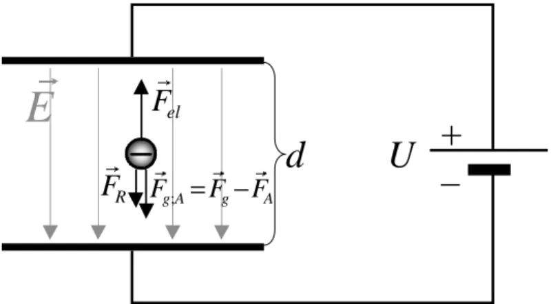
’s experiment consists of the observation of electrically charged oil droplets in be- tween two horizontal capacitor plates. The homogeneous electrical field ~ _E between the plates can be varied by applying a voltage U. Figure 1.1 shows a simplified sketch of the experimen- tal set-up using a negatively charged particle as an example.

U

E

F

F

A g A

g

F F

F

;

= − –

d +

Figure 1.1: Forces acting on a droplet: The weight force ~ _F

, the buoyant force ~ _F

_{, and the} friction force ~ _F

. When an electric field ~ _E is added by switching on a voltage U an additional Coulomb force ~ _F

_{is acting.}

In general, an electrically charged particle of mass m, volume V and charge Q will be influ- enced by the following forces:

1. The gravitational force F

= ρ

· _V · _g acts downwards. In contrast, the buoyancy the droplet experiences in air is aimed upwards and amounts to F

= ρ

· _V · _{g. We take} both forces into account by writing

~ _F

_: = ~ _F

− ~ _F

= ( ρ

− _ρ

) · _V · ~ g (1.1)

3

2. The polarity of the capacitor is such that the force applied to the oil droplets by the electrical field within the capacitor is aimed upwards. It amounts to

~ _F

= Q · ~ _E = Q U

d ~ e

(1.2)

Here, ~ _E is the electrical field, U is the voltage between the plates, d is their distance to each other and ~ e

is the unit vector perpendicular to the plates.

3. The air resistance counteracts the motion of the oil droplet and grows with its speed. We consider the oil droplet as a small ball in a laminar flow. Then the air resistance is given by the S

resistance:

~ _F

= − _6πrη ~ v (1.3)

Here, r is the radius of the droplet, v is its speed and η is the viscosity of air. Since the radius of the observed droplets is of the same order of magnitude as the mean free path of the air molecules, S

’ law only holds approximately. This needs to be taken into consideration when estimating the errors.

During the experiment, we observe oil droplets in three different stationary states:

1. Free fall in air resistance. The capacitor voltage is turned off. The force of gravity accelerates the droplet until it is compensated by friction and the droplet sinks with constant speed v

:

F

= F

( ρ

− _ρ

) · _V · _g = 6πrηv

(1.4) In the experiment we measure v

and thereby calculate the radius of the droplet r.

2. Rising under the influence of an electric current. Due to the relation between friction and speed, another stationary state is reached and the droplet moves upwards with constant speed v

:

F

+ F

= F

( ρ

− _ρ

) · _V · _g + 6πrηv

= Q U

d (1.5)

In the experiment we measure v

and use it together with r from equation (1.4) to deter- mine the charge Q of the droplet.

3. Floating state. If the voltage is chosen such that it compensates the gravitational force, the following holds:

F

= F

( ρ

− _ρ

) · _V · _g = Q U

d (1.6)

In the experiment we measure U

which again enables us to use r from (1.4) to determine the charge Q of the droplet.

4

1.2.2 Correction of the finite radius

Systematic investigations show that the experimentally determined value for the elementary charge e is slightly too big. The difference becomes larger at smaller radii of the observed oil droplets. This phenomenon can be traced back to Stokes’ law which is the basis for the analysis and does not hold exactly for the sizes of the encountered droplets. (The droplet radii lie roughly between 10

mm and 10

mm and thus in the order of magnitude of the mean free path of the air molecules.)

Correcting this is possible using a calculation already performed by M

.

If the corrected charge is denoted as Q

and the air pressure p (measured in mbar), the follow- ing equation holds (we neglect to derive it here):

Q

= ^Q

1 +

(1.7)

⇐⇒ _Q

= Q

·

1 + ^b r · _p

(1.8) b is a graphically quantifiable constant. Important to note here is that the number of elemen- tary charges on the droplet has a much greater influence on the measured charge than the correction factor we wish to find. After selecting the data points accordingly, equation (1.8) is a linear equation of the form

y = y

· ( 1 + bx )

Thus b is graphically quantifiable. In order to determine it, we proceed as follows: First, we draw y = Q

as a function of x =

; the resulting graph should look like a straight line that touches the ordinate at y

= Q

. Now we divide the slope of the line

by y

= Q

; the result is the constant b. (A good value for this constant is: b ≈ _{6, 33} · ₁₀

_mbar · _{m ) Once} b has been calculated, Q

can be determined by simply inserting it in equation (1.7).

1.3 Experiment

1.3.1 Material

Component Number

Millikan apparatus 1

Millikan operating device 1 Experiment cables 50cm, rot 1 Cable 50cm, red und blue 3

Cable 50cm, black 1

Camera 1

Computer 1

1.3.2 Set-up and alignment

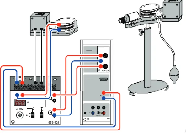
• Connect the capacitor and the lamp to the Millikan operating device as shown in 1.2.

(Make sure the plate capacitor is correctly polarized).

• As we limit ourselves to measurement method I in this experiment, we only need one stopwatch. Connect it to the designated output of the operating device.

• Familiarize yourself with the analyser program (see section 1.3.3).

5

Figure 1.2: On the left the schematic drawing of the set-up can be seen. The droplet chamber with the light source is at the top, the voltage supply is at the bottom on the left and the electronic stop watch is right next to it. On the very right side the Millikan apparatus can be seen.

• Oil droplets are sprayed into the chamber by a single push of the rubber ball (mind the oil level in the capillary).

• Check if the set-up shows the wanted behavior. Find out which direction is up, and down on the software.

Tip: In the absence of electric fields, in which direction the droplets should move?

• Wait a few seconds for air turbulence to settle after spraying the oil droplets.

• Adjust the current as necessary between 400-600V.

• Adjust the objective at the microscope until you see a sharp image of many droplets.

B

Please DO NOT change the distance between the lens and the camera. Please DO NOT use force or any screwdrivers

• Suitable droplets for the measurement carry at most 5 elementary charges (why?). They are the droplets that move the slowest in the electric field.

• Check the quality of the droplet to be measured by briefly turning the voltage off and on. Do not forget to reset the stopwatch to zero after doing so.

• At the end of the experiment, the oil sprayer needs to be covered again to prevent dust from accumulating in the oil with time.

6

1.3.3 Quick guide to use Toupview software

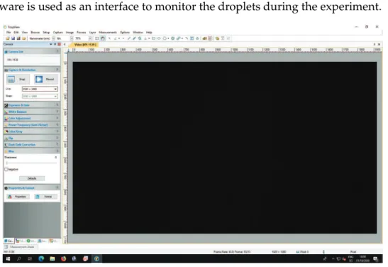
This software is used as an interface to monitor the droplets during the experiment.

Figure 1.3: The interface of the Toupview software. The camera can be chosen on the left at the top by clicking on HY-1139 (the name of the camera).

When you run the software for the first time, you should click on the camera’s name ("HY- 1139" on Fig. 1.3) from the camera list (top-left of the screen). This enables the camera.

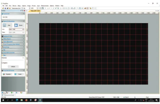
Next, you should choose "View">"Grids">"Auto Grids". This devides the screen in an equally spaced array. Note that the rulers on the top and left side of the window are in pixels. Hence, you can convert the distances to millimeters using the transformation ratio (given in section 1.3.4). For example, you might notice in the Figure 1.4 that the screen resolution is 1920 × ₁₀₈₀ pixel

(partitioned by a grid of 100 × _{100 pixel}

_).

1.3.4 Technical details

• Distance between capacitor plates: d = 6 mm

• Viscosity of air ( 20

C,760 Torr ) : η = 1, 81 · ₁₀

m²

• Density of the oil: ρ

= 875, 3

• Air density: ρ

( 0

C,760 Torr ) = 1, 293

Note: The air density depends on pressure and temperature. Regardless of that, ρ

( 0

C,760 Torr ) does not need to be converted to its value at room tem- perature since the following holds within measurement accuracy: ρ

≫ ρ

.

• Each setup is calibrated in a way that there is a transformation ratio to convert pixel distances to real distances:

Ratio of setup 1: r

= 711, 00 pixel/mm Ratio of setup 2: r

= 422, 56 pixel/mm

7

Figure 1.4: One can see the user interface after the grid is displayed. The grid can be found in the menu View at the top of the interface.

Measurements

We established in the theory part that there are two different ways to determine the elementary charge using ionized oil droplets in a capacitor:

1. Method of measurement I

• Determine the voltage U

at which the droplet just hovers

• Determine the fall speed v

without an electric field

• Determine the charge of the oil droplet from equations (1.4) and (1.6) 2. Method of measurement II

• Determine the fall speed v

without an electric field

• Determine the rise speed v

while applying an electric field

• Determine the charge of the oil droplet from equations (1.4) and (1.5)

Perform a series of measurements of a sufficiently large number of oil droplets for method I (n ≥ _50).

1.3.5 Tasks for the analysis

• Draw a first histogram for the results of the uncorrected droplet charge Q.

• Determine the Cunningham correction factor graphically.

• Draw a second histogram for the corrected charge distribution.

• Determine the elementary charge e by fitting (at most five) overlapping Gaussian func- tions (Show charge quantization).

8

• Discuss the result for e with respect to the measurement inaccuracy and compare with a literature value.

B

Please don’t forget to do the error estimations for the experiment.

1.4 Literature

• D. Meschede, ”Gerthsen Physik”, Springer Verlag

9