r
1
l2
2 1
m1
m2 l
ϕ ϕ y
x
g
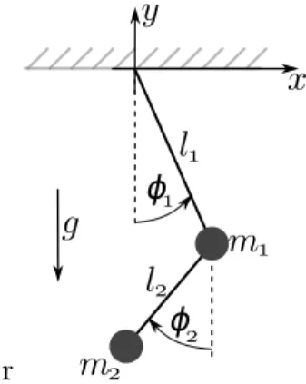
Figure 1: Double Pendulum
Physik auf dem Computer SS 2014
Worksheet 12: Solving differential equations
July 2, 2014
General Remarks
• The deadline for the worksheets isWednesday, 9 July 2014, 10:00for the tutorial on Friday and Friday, 11 July 2014, 10:00for the tutorials on Tuesday and Wednesday.
• On this worksheet, you can achieve a maximum of 10 points.
• To hand in your solutions, send an email to
– Johannes (zeman@icp.uni-stuttgart.de; Tuesday, 9:45–11:15) – Tobias (richter@icp.uni-stuttgart.de; Wednesday, 15:45–17:15) – Shervin (shervin@icp.uni-stuttgart.de; Friday, 11:30–13:00) Task 12.1: Double Pendulum (10 points)
In this task we consider a double pendulum with masses m1 = 1 and m2 = 1 attached by rigid massless wires of lengths l1= 1 and l2= 0.5 as it is shown in Fig. 1. Hereφ1 and φ2 are the angles between the wires and y-axis. The forces that act on the masses areF1 = −m1g and F2 =−m2g, respectively. For such a system the equation of motion can be written as a system of second order differential equations (1) that is derived from the Lagrangian equations. The trajectory of the mass m1 just falls on a circle, whereas the trajectory of the second mass m2 is chaotic. One can obtain the trajectories of both masses by solving the following system numerically:
M l1φ¨1+m2l2φ¨2cos(∆φ) +m2l2φ˙2
2sin(∆φ) +gMsinφ1 = 0 l2φ¨2+l1φ¨1cos(∆φ)−l1φ˙1
2sin(∆φ) +gsinφ2 = 0,
where M = (m1+m2) and ∆φ=φ1−φ2. .
1
• 12.1.1(2 points) Convert the equation system to a system of four differential equations of first order which will be suitable for using a Runge-Kutta method, i.e. ˙y=F[t, y(t)], wherey is the 4-vector (φ1,φ˙1, φ2,φ˙2). Implement a function F(t,y)that takes a 4-vector ywith angles and velocities and returns a 4-vector with F(t,y).
• 12.1.2 (3 points) Implement a Python function solve_runge_kutta(F,tmax,y0,h) that solves the double pendulum for a total time of tmax using the 4-th order Runge-Kutta method and returns the angles φ1 and φ2. Herey0consists of initial anglesφ1(0), φ2(0) and corresponding initial angular velocities ˙φ1(0), ˙φ2(0).
• 12.1.3 (3 points) Implement solve_velocity_verlet(F,tmax,y0,h), a Python function that solves the double pendulum for a total time of tmax using the Velocity-Verlet method. The arguments of the function are the same as in the previous subtask.
• 12.1.4(2 points) Using both implemented functions, solve the equation system withh= 0.01, tmax = 100 at the following initial conditions: φ1(0) =π/2,φ2(0) =π/2, ˙φ1(0) = 0, ˙φ2(0) = 0, in order to get the trajectory of the second mass m2 and plot the trajectory in x, y axes.
Compare the results of both methods.
2