Combined Faculties for the Natural Sciences and for Mathematics of the Rupertus Carola University of
Heidelberg, Germany for the degree of Doctor of Natural Sciences
presented by
Diplom-Geo¨okologe Olaf Ippisch born in F¨urth
Oral examination: 19th December, 2001
Porous Media
Referees: Prof. Dr. Kurt Roth
Prof. Dr. Peter Bastian
Da die Wechselwirkungen zwischen verschiedenen Transportprozessen f¨ur eine Reihe interessanter Systeme wichtig sind, wurde ein System partieller Differenti- algleichungen und effektiver Parameterfunktionen f¨ur die Untersuchung des gekop- pelten Wasser-, W¨arme-, Gas- und Stofftransportes formuliert und in einem State-of- the-Art Computermodell implementiert. Dabei wurde f¨ur die Beschreibung des ge- koppelten Gas-/Wassertransportes eine neue Druck/Druckformulierung entwickelt.
Mit dem Modell wurde der Wasser- und Energiehaushalt eines Permafrostbo- dens simuliert, wobei die wesentlichen Ph¨anomene reproduziert werden konnten.
Unterschiede lassen sich durch Heterogenit¨at und die Sensitivit¨at des Modells auf die ¨Anderung der hydraulischen Parameter erkl¨aren. W¨ahrend Wasserdampf- und Stofftransport keine Auswirkung auf das Ergebnis der Simulation hatten, erwies sich der Transport fl¨ussigen Wassers als wichtig f¨ur den Energietransport nahe dem Gefrierpunkt.
Bei der Untersuchung der Auswirkung der gew¨ahlten Parametrisierung und des verwendeten Modells auf die Simulation eines Multistep Outflow Experiments zeig- ten sich Unterschiede zwischen Richardsgleichung und Zweiphasen-Modell nur bei Verwendung einer Brooks-Corey Parametrisierung. Mit dem Zweiphasen-Modell er- gab sich dann eine langsamere Entw¨asserung und eine Hysterese beim Aufs¨attigen, was gut mit experimentellen Befunden ¨ubereinstimmt.
Coupled Transport in Natural Porous Media
As the interactions between transport processes are important for a number of interesting systems, a set of partial differential equations and appropriate para- meter functions for the study of coupled water, heat, gas and solute transport was formulated and a state of the art computer model for the numerical solution of the equation system was created. A new phase pressure/partial pressure formulation for the coupled transport of liquid and gas phase was developed.
The model was used to simulate the water and energy dynamics of a permafrost soil. A good qualitative agreement was achieved. Differences between modeled and measured data could be explained with heterogeneity in combination with the model’s sensitivity to a change in hydraulic parameters. Water vapor and solute transport had no effect on the simulation result but transport of liquid water proved to be an important heat transfer process near 0◦C.
The impact of the chosen parameterization and model on the simulation of a multistep outflow experiment was analyzed. Differences between a model based on Richards’ equation and a twophase model only occurred when the Brooks-Corey parameterization was used. The results of the twophase model showed a retarded drainage and a hysteresis during imbibation which is in good agreement with exper- imental results.
In our endeavor to understand reality we are somewhat like a man trying to under- stand the mechanism of a closed watch. He sees the face and moving hands, and even hears the ticking, but he has no way of opening the case. If he is ingenious enough he may form some picture of a mechanism which could be responsible for all the things he observes, but he may never be quite sure his picture is the only one which could explain his observations.
– Einstein and Infeld (1966) –
It is not possible to finish a research project like this without the help of a lot of people. So it’s time now to say thank you to
• Kurt Roth for his support, his many helpful suggestions and for many extended discussions (not only) about soil physics.
• Peter Bastian as he always had a helping hand when I got stuck with some numerical problems.
• Julia Boike, who is not only an excellent field scientist and a valuable colleague, but a close friend I would not want to miss.
• Hans-J¨org Vogel for lots of encouragement and professional support.
• Paul Ouverduin for great times in Ny ˚Alesund and San Francisco and the proof reading of this work.
• Hans Graf for the permission to use data measured at the ’HSPM’.
• Ute Wollschl¨ager. She often helped me to keep a realistic view.
• Marco Bittelli with whom I had some inspiring discussions about freezing soils.
• Hermann Lauer, Mihael Brajdic and G¨unter Balschbach for the assistance in the installation of a Linux cluster and in the common struggle against all types of computer problems.
• all colleagues at the University of Hohenheim and the Institut f¨ur Umwelt- physik in Heidelberg.
• the Alfred-Wegener-Institute.
• all my personal friends, who helped me through some difficult times.
• the “unknown helper” as a substitute for all the people I forgot to mention.
Finally I’d like to thank my family. Without their support it would not have been possible for me to finish my study.
This work was done as part of a research project supported by the Deutsche Forschungsgemeinschaft (Ro 1080/4-1&2).
Zusammenfassung i
Summary i
Acknowledgments iii
List of Figures ix
Notation xii
1 Introduction 1
2 Theory of Coupled Transport Processes in Porous Media 3
2.1 System Description . . . 3
2.2 Basic Considerations . . . 4
2.2.1 Continuum Approach . . . 4
2.2.2 Representative Elementary Volume . . . 6
2.2.3 Further Assumptions . . . 7
2.3 Balance Equations . . . 7
2.3.1 Storage Terms . . . 8
2.3.2 Flux Laws . . . 9
2.3.3 Multiphase Transport and Richards’ Equation . . . 11
2.4 Effective Parameters . . . 11
2.4.1 Soil Water Characteristic . . . 11
2.4.1.1 Temperature Dependence . . . 12
2.4.1.2 Gas Phase Saturation . . . 13
2.4.1.3 Freezing Curve . . . 13
2.4.2 Gas and Liquid Phase Conductivity . . . 15
2.4.3 Diffusion Coefficients . . . 17
2.4.4 Water/Solute Interaction . . . 18
2.4.5 Fluid/Gas Properties . . . 19
2.4.5.1 Gas Solubility . . . 19
2.4.5.2 Viscosity of Liquid and Gas Phase . . . 20
2.4.5.3 Densities . . . 20
2.4.6 Heat Conductivity . . . 21
2.4.6.1 Water Vapor Transport . . . 22
2.4.7 Mechanical Interactions . . . 26
3 Numerical Solution 28 3.1 Mathematical Formulation of the Equation System . . . 28
3.1.1 Phase Pressure/Saturation Formulation . . . 28
3.1.2 Partial Pressure/Phase Pressure Formulation . . . 29
3.2 Discretization . . . 30
3.2.1 Spatial Discretization . . . 30
3.2.1.1 Heterogeneity . . . 33
3.2.1.2 Boundary Conditions . . . 33
3.2.2 Time Discretization . . . 34
3.3 Solution of the Nonlinear Equation System . . . 35
3.4 Solution of the Linear Equation System . . . 35
3.5 Process Coupling . . . 36
3.6 Variable Substitution . . . 36
3.7 Time Stepping . . . 37
3.8 Testing and Verification . . . 38
3.8.1 Mass Balances . . . 38
3.8.2 Comparison with Analytical Solutions . . . 38
3.8.2.1 Water Transport . . . 39
3.8.2.2 Heat-/Solute-/Gas Transport . . . 40
4 Application: Simulation of a Permafrost Soil 46 4.1 Dynamics of Permafrost Soils . . . 46
4.2 Field Experiment . . . 47
4.2.1 Instrumentation . . . 47
4.2.2 Data Preparation . . . 50
4.2.3 Climate . . . 52
4.2.4 Model Parameters . . . 53
4.2.4.1 Transport Parameters . . . 53
4.2.4.2 Pseudo-Mechanical Submodel . . . 55
4.2.4.3 Boundary Conditions . . . 56
4.2.4.4 Initial Conditions . . . 59
4.3 Simulation Results . . . 59
4.3.1 Homogeneous Simulations . . . 60
4.3.1.1 Numerical Tests . . . 63
4.3.1.2 Relevance of Different Heat Transport Processes . . . 64
4.3.1.3 Solute Transport . . . 66
4.4 Heterogeneous Simulation . . . 67
4.5 Discussion . . . 67
5 Application: Multiphase Transport 69 5.1 Multistep Outflow Experiments . . . 69
5.2 Laboratory Experiments . . . 70
5.3 Model Parameters . . . 70
5.3.1 Transport Parameters . . . 70
5.3.2 Initial and Boundary Conditions . . . 71
5.4 Simulation Results . . . 71
5.4.1 Homogeneous Medium . . . 72
5.4.2 Heterogeneous Medium . . . 73
5.5 Discussion . . . 76
6 Conclusions 79 Bibliography 81
Appendix 89
A Hydraulic Parameters for the Test Calculations 90 A.1 Yolo Light Clay . . . 90A.2 Sand . . . 90
B Texture and Composition of the Bayelva Profile 91 C Algorithm for the Evaluation of TDR-traces 92 D Freezing Curves 94 E Simulation Results 96 E.1 Measured Data . . . 97
E.2 Loam/Silt Homogeneous . . . 99
E.3 Loam/Silt with Reduced Permeability . . . 101
E.4 Loam Freezing/not Freezing . . . 103
E.5 Loam Coarse Grid/Fine Grid . . . 105
E.6 Loam with Different Initial Conditions . . . 107
E.7 Loam with Dirichlet Boundaries at the Sides . . . 109
E.8 Loam with 2m deep Lower Boundary . . . 111
E.9 Loam 3D Simulation . . . 113
E.10 Loam without Vapor Transport . . . 115
E.11 Loam with Vapor Transport Formulated According to Philip and de Vries . . . 117
E.12 Loam with Inclusion of Solute Transport . . . 119 E.13 Heterogeneous Simulation . . . 121
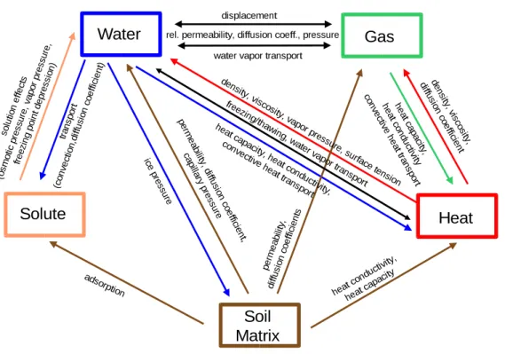
2.1 The main elements of a natural porous medium and their interactions
as considered in this work . . . 4
2.2 Schematic representation of a porous medium at pore scale and con- tinuum scale . . . 6
2.3 Change of hydraulic conductivity with increasing averaging volume . 7 2.4 Molar enthalpy of the phase change liquid water/ice resulting from the balance equation and fitted to measured values . . . 9
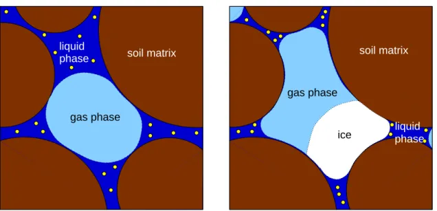
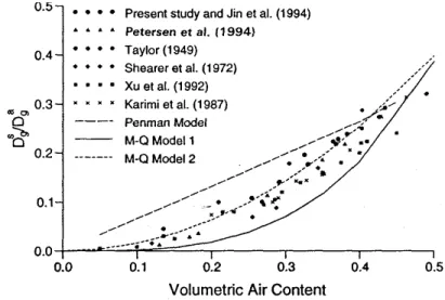
2.5 Schematic representation of the pore space before and after freezing . 14 2.6 Comparison of measured relative diffusion coefficients with different tortuosity models . . . 19
2.7 Example for the dependence of the heat conductivity of a porous medium on ice and water saturation calculated with the generalized de Vries model . . . 22
2.8 Water vapor transport through a liquid island . . . 24
2.9 Temperature distribution in a simple heterogeneous medium . . . 25
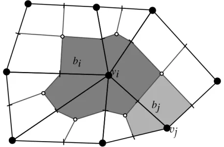
3.1 Element mesh and control volumes . . . 31
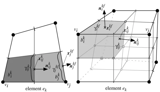
3.2 Elements with sub-control volumes . . . 32
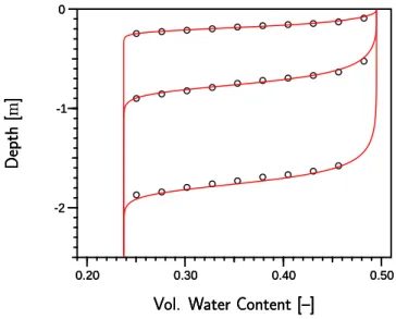
3.3 Comparison of profiles calculated with the model and with Philip’s quasianalytical solution for the Yolo Light Clay . . . 40
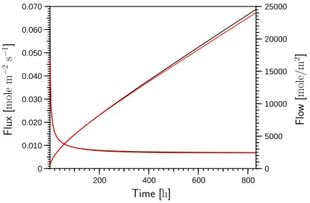
3.4 Comparison of infiltration rates and cumulative infiltration calculated with the model and with Philip’s quasianalytical solution for the Yolo Light Clay . . . 41
3.5 Comparison of profiles calculated with the model and with Philip’s quasianalytical solution for the sand . . . 41
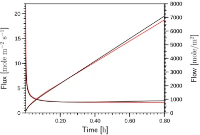
3.6 Comparison of infiltration rates and cumulative infiltration calculated with the model and with Philip’s quasianalytical solution for the sand 42 3.7 Comparison of the simulated partial pressure of air and solute con- centration profiles and the analytical solution with pure diffusion . . . 44
3.8 Comparison of the simulated temperature profile and the analytical solution with pure heat conduction . . . 44
3.9 Comparison of the simulated partial pressure of air and solute con- centration profiles and the analytical solution with convection . . . . 45
3.10 Comparison of the simulated temperature profile and the analytical
solution with pure heat conduction . . . 45
4.1 View from Leirhaugen hill southward over the Bayelva catchment toward the East Brøggerbreen glacier . . . 48
4.2 Surface of the selected unsorted circle before instrumentation . . . 49
4.3 Soil profile of the unsorted circle . . . 49
4.4 Aerial view of the field site in April 2000 . . . 50
4.5 Comparison of the relative permittivity determined by the datalogger algorithm and the modified Heimovaara algorithm . . . 51
4.6 Data measured at a TDR-probe before and after filtering, interpola- tion and smoothing . . . 52
4.7 Air temperature and humidity at the Bayelva site . . . 52
4.8 Snow depth and precipitation at the Bayelva site . . . 53
4.9 Solar and net radiation at the Bayelva site . . . 53
4.10 Freezing characteristic for three representative probes . . . 55
4.11 Positions of the probes used in the simulation . . . 57
4.12 Plot of 3D domain with a cross section showing temperature . . . 58
4.13 Temperature and relative permittivity profiles during thawing . . . . 61
4.14 Temperature and relative permittivity profiles during freezing . . . . 62
4.15 Simulated cumulative flow of water over the upper and lower bound- ary in the loam scenario . . . 63
4.16 Simulated heat flux over the upper and lower boundary in the loam scenario . . . 64
4.17 Effective heat transport due to liquid water flux . . . 65
4.18 Profiles of temperature, ice saturation, liquid phase pressure, water saturation, phase state, relative permittivity, water flux and heat flux. Values in brackets are the maximum and minimum values used in scaling 66 5.1 Heterogeneous test column composed of sintered glass with fine, me- dium and coarse pores . . . 70
5.2 Soil water characteristic for the coarse, medium and fine material using the van Genuchten and Brooks-Corey parameterization . . . 72
5.3 Outflow of water calculated with Richards’ equation and the twophase model obtained with the van Genuchten parameterization for the ho- mogeneous column made of medium material . . . 74
5.4 Outflow of water calculated with Richards’ equation and the twophase model obtained with the Brooks-Corey parameterization for the ho- mogeneous column made of medium material . . . 74
5.5 Outflow of water calculated with Richards’ equation and the twophase model obtained with the van Genuchten parameterization for the het- erogeneous column . . . 75
5.6 Outflow of water calculated with Richards’ equation and the twophase model obtained with the Brooks-Corey parameterization for the het- erogeneous column . . . 75 5.7 Distribution of liquid phase pressure, gas pressure, water saturation,
gas saturation and fluxes in the heterogeneous column after 5 hours . 77 5.8 Distribution of liquid phase pressure, gas pressure, water saturation,
gas saturation and fluxes in the heterogeneous column after 6 hours . 77 5.9 Relative permeabilities for gas phase and liquid phase for the medium
material . . . 78 C.1 TDR waveform for a probe immersed in water, its first derivative
and the regression lines for the determination of the first and second reflection. . . 92 E.1 Positions of the probes used in the simulation . . . 96
Scalar values, functions and sets are denoted by normal letters (e.g. pl, kr, Si, . . .).
Vectors are typeset in boldface symbols (e.g. x), whereas tensors are written in boldface italic letters (e.g. K).
Lowercase Latin Symbols
bi,bj Control volumes bki, bkj Sub control volumes
∂bi Boundary of control volume i
cal Concentration of dissolved air in the liquid phase [mole/m3] csl Concentration of solute in the liquid phase [mole/m3]
csli Concentration of solute species iin the liquid phase [mole/m3] cwl Concentration of water in the liquid phase [mole/m3]
e1,. . . ,ek Elements ej Unity vector
fSi Damping parameter of ice on liquid phase permeability [–]
ga, gb, gc Form factors for the de Vries model [–]
hm Matrix head [m]
ja Molar air flux [mole m−2 s−1] je Energy flux [W/m−2]
jconve l Convective energy flux in the liquid phase [W/m−2] jconve g Convective energy flux in the gas phase [W/m−2] jlate Latent heat flux [W/m−2]
jconde Conductive energy flux [W/m−2]
jgi Total flux of component iin the gas phase [mole m−2 s−1] jli Total flux of component iin the liquid phase [mole m−2 s−1] jgiD Molar flux of componenti in the gas phase due to molecular
diffusion [mole m−2 s−1] jNk Flux at Neumann boundary js Molar solute flux [mole m−2 s−1] jw Molar water flux [mole m−2 s−1]
kH Henry coefficient for oxygen [Pa]
kNH2 Henry coefficient for nitrogen [Pa]
kiH Henry coefficient of gas i [Pa]
ki Ratio of the average temperature gradient in particles of type i to the average temperature gradient in the surrounding medium [–]
krg Relative permeability of the gas phase [–]
krl Relative permeability of the liquid phase [–]
krl
hf Relative permeability of the high flow domain [–]
n Van Genuchten parameter [–]
nkij Outward directed normalized vector normal to γijk m Van Genuchten parameter [–]
pad Capillary pressure above which adsorption forces are prevalent [Pa]
patm Gas pressure in the free air above the soil [Pa]
pcap Capillary pressure below which capillary forces are prevalent [Pa]
pag Partial pressure of air [Pa]
pc Capillary pressure [Pa]
pe Air entry pressure [Pa]
pg Gas phase pressure [Pa]
pwg Partial pressure of water [Pa]
pl Liquid phase pressure [Pa]
pig Partial pressure of gas i [Pa]
qa Air source/sink term [mole m−3 s−1] qe Energy source/sink term [W/m−3] ql Volumetric liquid phase flux [m3/s]
qs Solute source/sink term [mole m−3 s−1] qw Water source term [mole m−3 s−1] r Pore radius [m]
rH Humidity [–]
t Time [s]
vl Pore water velocity [m/s]
vlw Molar volume of liquid water [m3/mole]
viw Molar volume of ice [m3/mole]
xi Position of vertex i
xkij Barycenter of sub-control volume face i
z Height [m]
z0 Reference height [m]
Uppercase Latin Symbols
A Flux term
Cs Volumetric heat capacity of the matrix [J m−3 K−1] Cga Molar heat capacity of air [J mole−1 K−1]
Cgw Molar heat capacity of water vapor [J mole−1 K−1] Ciw Molar heat capacity of ice [J mole−1 K−1]
Clw Molar heat capacity of liquid water [J mole−1 K−1]
Dig Dispersion coefficient of component i in the gas phase [m2/s]
Dil Dispersion coefficient of component i in the liquid phase [m2/s]
Dijg Binary diffusion coefficient of components i and j in the gas phase [m2/s]
DwgT Diffusion coefficient for water vapor transport due to a temperature gradient [mole m−1 s−1 K−1]
Dwgpc Diffusion coefficient for water vapor transport due to a moisture gradient [mole s m−1 kg−1]
Dwgatm Diffusion coefficient for water vapor transport in free air [m2/s]
E Energy density [J/m3]
Fijk Area of sub-control volume face [m2]
∆Hlgw Molar phase change enthalpy of water vapor at reference temperature [J/mole]
∆Hilw Molar phase change enthalpy of ice at reference temperature [J/mole]
J Jacobi matrix
Jg Volumetric convective flux of the gas phase [m/s]
Jl Volumetric convective flux of the liquid phase [m/s]
Kl Hydraulic conductivity [m3 s kg−1] Kg Gas phase conductivity [m3 s kg−1]
M Storage term
Mi Molar mass of component i [kg/mole]
Mw Molar mass of water [kg/mole]
Q Source term
R Ideal gas constant [J mole−1 K−1] S Saturation [–]
Seg Effective gas phase saturation [–]
Sel Effective liquid phase saturation [–]
Sg Gas phase saturation [–]
Si Ice phase saturation [–]
Sl Liquid phase saturation [–]
Slhf Liquid phase saturation of the high flow domain [–]
Srg Residual gas phase saturation [–]
Si Entropy of ice [J/K]
Stotw Total water saturation (liquid water plus ice) [–]
T Temperature [K]
Vik Volume of sub-control volume [m3]
(∇T)g Average temperature gradient in the gas phase [K/m]
Xlw Molar fraction of water in the liquid phase [–]
Xi Volumetric fraction of component i [–]
Xli Molar fraction of gas i in the liquid phase [–]
Lowercase Greek Symbols
α Van Genuchten parameter [Pa−1] α Exponent in mixing formula [–]
αh Heat exchange parameter [W m−2 K−1] χg Stress partition factor for the gas phase [–]
χi Stress partition factor for the ice phase [–]
χl Stress partition factor for the liquid phase [–]
²a Relative permittivity of air [–]
²i Relative permittivity of ice [–]
²m Relative permittivity of the soil [–]
²s Relative permittivity of the soil matrix [–]
²w Relative permittivity of water [–]
ηi Parameter function γ Contact angle [–]
γijk Sub control volume face λ Brooks-Corey parameter [m]
λ Heat conductivity [W m−1 K−1]
λ0 Heat conductivity of the surrounding medium [W m−1 K−1] λi Heat conductivity of component i[W m−1 K−1]
λ∗ Heat conductivity of a soil without vapor transport [W m−1 K−1] λeff Effective heat conductivity of a soil [W m−1 K−1]
µl Dynamic viscosity of the liquid phase [Pa s]
µg Dynamic viscosity of the gas phase [Pa s]
νa Total molar density of air [mole/m3]
νga Molar density of air in the gas phase [mole/m3] νs Total molar density of solute [mole/m3]
νw Total molar density of water [mole/m3]
νgw Molar density of water in the gas phase [mole/m3] νiw Molar density of ice [mole/m3]
νgw0 Molar density of saturated water vapor above a solution [mole/m3] νgw•0 Molar density of saturated water vapor above pure water [mole/m3] νgi Molar density of componenti in the gas phase [mole/m3]
φi Nodal basis functioni
ψg Gravitational potential [J/m3] ρg Density of the gas phase [kg/m3] ρl Density of the liquid phase [kg/m3] ρwl Density of liquid water [kg/m3] σe Effective stress [Pa]
σn Neutral stress [Pa]
σla Surface tension of the liquid phase/air phase interface [J/m2] θw Volumetric water content [–]
τ Tortuosity in the Mualem model [–]
υi,υj Vertices
ξ Tortuosity factor [–]
ξg Tortuosity factor for the gas phase [–]
Uppercase Greek Symbols
Γ Model boundary
Ω Model domain
Φ Porosity [–]
Πo Osmotic pressure [Pa]
Norms, Operators
∇ Divergence operator
∇ Gradient operator
Indices
e Energy
g, l, i Gas, liquid, ice phase s Soil matrix
a,w,i, s Components: air, water, ice, solute
k Control volume
n Index for discretized time
Coupled transport processes are important for two rather different but neverthe- less very relevant environmental problems: Global warming and the pollution of groundwater.
Water, heat and solute transport processes are strongly coupled in freezing or thawing soils. As a significant part of the earth’s continental area (∼ 25 % of the exposed land surface in the Northern Hemisphere, Zhang et al. 1999) is underlain by permafrost1 and permafrost soils are an important storage of organic carbon and methane, a thawing of wide areas could lead to a dangerous feedback for global climate change (Goulden et al. 1998). A 12 to 15 % reduction of the near-surface permafrost area and a 15 to 30 % increase of the active layer2 thickness is indicated by recent modeling studies (Anisimov and Nelson 1996, Anisimov and Nelson 1997, Anisimov et al. 1997) for the middle of the 21st century. For the prediction of the future development of climate, the understanding of the water and heat dynamics of permafrost soils is therefore of great significance. The possibility to simulate the response of permafrost soils to global warming would facilitate reliable climate predictions.
Many permafrost soils are heterogeneous due to slow weathering and periglacial mixing processes in cool climates. An adequate description therefore requires at least two-dimensional models. However most of the models commonly used are either one-dimensional (Nakano and Brown 1972, Jansson 1998, Flerchinger and Saxton 1989, Padilla and Villeneuve 1992, Shoop and Bigl 1997, Zhao et al. 1997) or they are intended for the modeling of frost heave and ice lense development and have a simplified description of water and energy transport (O’ Neill and Miller 1982, Fowler and Krantz 1994, Selvadurai et al. 1999, Li et al. 2000).
Another problem of great environmental and economic importance is the pollution of groundwater. Computer models based on Richards’ equation (Richards 1931) are often used to predict the transport of dissolved chemicals (especially pesticides, fertilizers and heavy metals). However, the interaction of gas phase and liquid phase is assumed to be negligible in the derivation of Richards’ equation. This is not true
1Permafrost is defined as ground or substrate that is continuously below 0 ◦C for two or more years (National Research Council of Canada 1988).
2The active layer is the temporarily unfrozen part at the surface of a permafrost soil.
at high water saturations, which can occur during infiltration events and are of great importance for the transport of contaminants.
The objective of this study is the development of a flexible, stable and robust model with state-of-the-art numerical solvers to study the coupled water, heat, so- lute and gas transport in frozen and unfrozen soils at the laboratory to plot scale.
Two- and three-dimensional simulations must be possible in order to represent the heterogeneity of a soil. Although mechanical processes are important in freezing soils, they are not considered explicitly, as this would be beyond the scope of this study. However, the possibility to integrate a mechanical model later was accom- modated in the development. The model is used to simulate the heat and water dynamics of a permafrost site near Ny ˚Alesund, Spitsbergen and of laboratory ex- periments commonly used to estimate the water transport properties of soils.
Processes in Porous Media
A set of equations for the description of coupled mass and energy transport in frozen and unfrozen soil and porous media is developed in this chapter. A discussion of basic concepts is followed by the formulation of balance equations, flux laws and the specification of parameter functions.
2.1 System Description
Soils are complex dynamic entities. The soil surface usually has some microrelief and is covered by different types of vegetation. Horizontal layers, soil horizons, of varying size and extension can be seen in the soil profile. The horizons are often composed of lumps of material called aggregates separated by a network of pores. The aggregates themselves are a mixture of different mineral components with smaller pores in between. Water, heat and solutes are transported, ions and organic molecules adsorbed and released, minerals are decomposed and newly created, and the soil is populated by an incredible variety of bacteria, insects and animals. Under the influence of climate, the soil structure is changed by swelling and shrinking, freezing and thawing.
In this study soil is envisaged as a porous medium composed of a solid matrix and an interconnected pore space filled with water, air and solutes. Water, solutes and dissolved air (the consideration of dissolved air is necessary to solve some numerical difficulties) form the liquid phase1 and the gas phase consists of air and water vapor.
The components2 are transported by diffusion and convective transport processes in liquid and gas phase. Energy is associated with the heat capacity of the components
1A phase is defined as a “chemically and physically uniform or homogeneous quantity of matter that can be separated mechanically from a nonhomogeneous mixture and that may consist of a single substance or of a mixture of substances” (Encyclopaedia Britannica 2001). In this study, besides the soil matrix, a liquid, gas and ice phase are considered
2A component is defined by Bear and Bachmat (1991) as part of a phase that is composed of an identifiable homogeneous chemical species or of an assembly of species (ions, molecules). The three components water, air and one solute are used in this work.
Water Gas
Solute
Soil Matrix
Heat
displacement
water vapor transport
solution effects
(osmotic pressure, vapor pressure, freezing point depression)
transport
(convection,diffusion coefficient)
adsorption ice
pre ssu
re pe
rmeab ility, d
iffusion coe
fficien t, cap
illary pre
ssu re
heat ca pacity, h
eat con ductivity, convective
heat trans port freezing
/thawin g, wate
r vapor transport density
, viscos ity, v
apor pressu re, s
urface tension den
sity, visco
sity, diffu
sion coe
fficient hea
t capa city, hea
t condu ctivity con
vective hea
t tran spo
rt
perm eability,
diffusion coefficients
heat conductivity, heat capacity rel. permeability, diffusion coeff., pressure
Figure 2.1: The main elements of a natural porous medium and their interactions as considered in this work
and the phase change of water. Mass movements and heat conduction transport energy. Figure 2.1 shows the main elements and their interactions.
For simplicity, a detailed analysis of solute transport is not performed. Only the transport of one solute, representing ionic strength, is taken into account. Mechan- ical interactions are also not considered in detail. Although they might be quite important in freezing porous media, the complexity of the interactions is beyond the scope of this work.
2.2 Basic Considerations
2.2.1 Continuum Approach
The observable phenomena and their description are closely linked to the resolution with which an porous medium is analyzed. At least three scales can be distinguished.
Molecular scale
At the molecular scale the interactions between individual atoms and molecules in the pore space and the solid material are treated explicitly. Interesting variables
are the velocity and mass of the molecules, their rotation, and the distribution of electrical charges. Interaction is dominated by electrical forces either on large distances if charged particles or surfaces are involved, or in the short range, when atoms or molecules collide.
Pore scale
The motion of individual molecules can be averaged, if the mean free path length3 is much larger than the scale of interest. Positions, velocities and molecular masses are replaced by continuous state variables like density, pressure or temperature.
Regions with a distinct change in state variables (e.g. in density: liquid/gas) are called phases. In a porous medium normally more than one phase coexist (gas phase/liquid phase/solid phase). Molecules may be able to change from one phase to another.
If the mean free path length is large compared to the pores of the solid, trans- port can be described by Knudsen diffusion. Interactions between molecules in the pore space and the solid material (including the geometry of the solid material) are lumped into the Knudsen diffusion coefficient.
If the mean free path length is much smaller than the pore diameter, the Navier- Stokes equations can be applied. The average interactions between molecules in the mobile phase are described by the effective parameters viscosity and diffusion coefficient. The surface properties and geometry of the pore space must be treated by appropriate boundary conditions. High resolution measurements of the geometry of the pore space are limited to small sample volumes. The speed of available computers also sets tight bounds to the size of a sample which can be simulated with a pore scale model.
Continuum scale
On the continuum scale phases are treated as continuous fields. At each point of space there are no longer distinct phases, but fractions of different phases. The phases are not mixed but microscopic geometry is no longer resolved (Figure 2.2).
Phase boundaries and the geometry of the pore space are taken into account by new effective parameters like permeability. Transition from pore scale to continuum scale is possible if the pore space is either homogeneous above a certain scale or heterogeneities are hierarchical. The applicability of a continuum scale model for porous media is therefore closely linked to the existence of a so called “representative elementary volume” (REV).
3The mean free path length is defined as the mean distance a molecule travels before hitting another molecule
Figure 2.2: Schematics representation of a porous medium at pore scale (left) and continuum scale (right)
2.2.2 Representative Elementary Volume
If a horizontal pressure gradient in x-direction is applied to a water saturated soil column, the water transport is often described with Darcy’s law (Darcy 1856):
ql=−Kl·∂ pl
∂ x, (2.1)
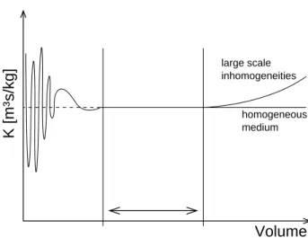
where ql is the volumetric flux, Kl is a material specific parameter called hydraulic conductivity and pl is the liquid phase pressure. If we know the flux and pressure field at the pore scale, we can calculateKl at a certain position by averaging over a certain volume. If the averaging volume is gradually increased, we might get a result similar to figure 2.3. For small averaging volumes the variations are quite large, as changes of velocity and pressure can be very large at small distances (either large pores, small pores or solid material are included). With increasing volume less new information is incorporated. The variations are getting smaller until a plateau may be reached. If we increase the volume even further the value might change again, because of large scale heterogeneities. The plateau exists only, if the pore space is homogeneous at least at some intermediate scale. The smallest volume at which the average value does no longer change significantly with changing averaging volume is called “representative elementary volume” (cf. Bear 1972).
The REV can be different for different effective parameters (porosity, hydraulic conductivity, . . . ). Transport in a porous medium can only be described at the continuum scale, if a common REV for all necessary effective parameters exists.
In general the existence of an REV can not be proven easily for a specific porous medium. The applicability of a macroscale description must be verified by compar- ison of results from experiment and simulation.
large scale inhomogeneities
homogeneous medium
Volume
K [m³s/kg]
Figure 2.3: Change of hydraulic conductivity with increasing averaging volume. The conductivity is essentially constant in the marked interval
Heterogeneity due to changes of composition or pore space geometry at a larger scale can be considered by using different sets of effective parameters for each re- gion. Effective parameters can also have tensorial character (e.g. permeability) to represent directional differences in the structure of the pore space.
2.2.3 Further Assumptions
The following basic assumptions are made in the description of the system:
• Air can be treated as a single gas. Oxygen, nitrogen and carbon dioxide are not treated separately. Air and water vapor are assumed to be ideal gases.
• Dissolved air and the modeled solute can be considered to be ideal solutes. In the solution they behave exactly like water molecules.
• Local thermodynamic equilibrium is assumed. Kinetic effects are not taken into account.
2.3 Balance Equations
To derive continuum scale transport equations, the principle of mass and energy conservation is used to formulate balance equations for each component.
For a non-isothermal system consisting of water, gas and one solute we get a system of four partial differential equations:
∂ νw
∂t +∇ ·jw =qw (2.2)
∂ νa
∂t +∇ ·ja=qa (2.3)
∂ νs
∂t +∇ ·js=qs (2.4)
∂E
∂t +∇ ·je =qe (2.5)
with νw,νa,νs: Molar density of water, air, solute [mole/m3] E: Energy density [J/m3]
jw, ja,js: Molar flux (water/air/solute) [mole m−2 s−1] je: Energy flux [W/m−2]
qw, qa, qs: Source/sink term (water/air/solute) [mole m−3 s−1] qe: Energy source/sink term [W/m−3]
2.3.1 Storage Terms
The total mass of a component is calculated as sum over the phases. If we assume that the gas phase is composed of water vapor and air, the liquid phase of water, solute and dissolved air and the ice phase of pure water, we get the storage terms:
νw = Φ·³Sg·νgw+Sl·cwl +Si·νiw´ (2.6)
νa = Φ·³Sg·νga+Sl·cal´ (2.7)
νs = Φ·Sl·csl (2.8)
with Φ: Porosity [–]
Sg,Sl, Si: Phase saturation4 (gaseous/liquid/ice) [–]
νgw,νga: Molar density of water and air in the gas phase [mole/m3]
cwl , cal, csl: Concentration5 of water, air, solute in the liquid phase [mole/m3] νiw: Molar density of ice [mole/m3]
Energy storage can be computed from porosity, phase saturations and the heat capacity of the components. As we use liquid water at 0 ◦C as reference state, the phase change enthalpy of water vapor and ice must be taken into account as well.
If we use the phase change enthalpies at the reference temperature in this storage equation, the phase change enthalpy varies with temperature in the model due to the different heat capacity of ice, water and vapor. Figure 2.4 shows a comparison of the resulting temperature dependence of the phase change enthalpy of ice with a formula fitted to experimental results (Spaans and Baker 1996). As we assume an
4The saturation is defined as the fraction of pore space occupied by a phase.
5The term concentration is used instead of the term molar density in solutions, as the concentra- tion also depends on the composition of the liquid phase.
5200 5400 5600 5800 6000 6200
255 260 265 270
! #"%$&')(+*-,
Figure 2.4: Molar enthalpy of the phase change liquid water/ice resulting from the balance equation (dashed line) and fitted to measured values (solid line) ideal solution, dissolved molecules behave like water molecules and the molar heat capacities Cla, Cls and Clw are identical.
E = T ·nΦ·hSlClw(cwl +cal +csl) +Sg³Cgaνga+Cgwνgw´+SiCiwνiwi +(1−Φ)·Cs
o+ ∆HlgwΦSgνgw−∆HilwΦSiνiw (2.9)
with T: Temperature [K]
Clw, Cgw, Cga, Ciw: Molar heat capacities (liquid water,vapor,air, ice) [J mole−1 K−1]
Cs: Volumetric heat capacity of the matrix [J m−3 K−1]
∆Hlgw, ∆Hilw: Molar phase change enthalpies of water vapor and ice at reference temperature [J/mole]
2.3.2 Flux Laws
The formulation of flux laws is a central step in the development of a model. One possibility is the definition of a potential for every component and the calculation of the flux as product of the negative gradient of the potential and an effective parameter. For water the “hydraulic potential” is defined as the energy difference between bound water in a porous medium with dissolved solutes and free, pure water at a reference height. However this potential can hardly be measured and as an integral quantity it is also difficult to calculate. The gravitational potential for example is usually (e.g. Kutilek and Nielsen 1994) given as ψg = ρwl g(z −z0).
This is only correct if the density of water is constant. If the density varies, a term g(z −z0)∇ρwl would occur in ∇ψg besides the gravity force ρwl gez, where ez is the
unity vector in z-direction. The correct expression for ψg in the case of varying density is Rzz0ρwl (z)gdz.
An alternative approach specifies the transport processes and relates them to gradients of state variables which can be measured. Water for example is transported by convection6 driven by gravity and the gradient of liquid phase pressure, and by diffusion7. In laboratory experiments the liquid phase pressure can be measured with tensiometers and pressure transducers. At very low water contents water is transported in liquid films on solid surfaces. As this is normally included into the calculation of convection, the liquid phase pressure may also become negative. This reminds us that further research on water transport in very dry porous media is needed. The resulting transport equations are:
Jl = −Kl(Sl)·(∇pl−ρl·g) (2.10)
jli = cil·Jl−Dil· ∇νli (2.11)
Jg = −Kg(Sg)·(∇pg−ρg·g) (2.12)
jgi = νgi ·Jg−Dig· ∇νgi (2.13)
with Jg, Jl: Volumetric convective flux of the gas/liquid phase [m/s]
ρl= P
i=w,a,scilMi: Density of the liquid phase [kg/m3] ρg = P
i=w,aνgiMi: Density of the gas phase [kg/m3] Mi: Molar mass of component i [kg/mole]
Kl(Sl),Kg(Sg): Liquid/gas phase conductivity tensor [m3 s kg−1] pl: Liquid phase pressure [Pa]
pg = P
j=w,apjg: Gas phase pressure [Pa]
pwg,pag: Partial pressure of water/air [Pa]
g: Acceleration of gravity [m/s2]
jli, jgi: Total flux of component i in the liquid/gas phase [mole m−2 s−1]
Dli,Dig: Dispersion coefficient of component i in the liquid/gas phase [m2/s]
Equation 2.10 is equivalent to the Darcy-Buckingham-Equation (Buckingham 1907).
Energy is transported either by convection of the gas and liquid phase, as latent heat with water vapor or by heat conduction. This processes can be described by (de Vries 1958):
je =jconve l+jconve g +jlate +jconde (2.14)
6Convection is defined as transport of a phase as a whole
7Diffusion is defined as transport of molecules, resulting from concentration gradients, relative to a frame of reference in which the phase as a whole is stationary
where
jconve l = T ·Clw ·Jl (2.15)
jconve g = T · X
i=w,a
Cgi ·jgi (2.16)
jlate = ∆Hlgw ·jgw (2.17)
jconde = −λ(Sl, Sg)· ∇T (2.18)
with λ(Sl, Sg): Heat conductivity [W m−1 K−1].
2.3.3 Multiphase Transport and Richards’ Equation
Liquid and gas phase transport are coupled as they share the same pore space. Due to its smaller viscosity, the gas phase is much more mobile than the liquid phase.
It is often assumed that the gas phase is mobile enough to be always (nearly) at atmospheric pressure and to be no obstacle to the liquid phase flow. Gas and liquid phase transport can then be decoupled. The result is Richards’ equation (Richards 1931), which is identical to the combination of equations 2.2, 2.6 and 2.10 ifpg =patm
is used in the calculation of Sl.
2.4 Effective Parameters
To fill the flux laws and balance equations with life, we have to specify the effective parameters used in the calculation of storage terms and in the flux laws.
2.4.1 Soil Water Characteristic
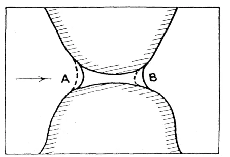
In experiments a strong relationship between the water content of a porous medium and the pressure difference between liquid and gas phase is observed. This relation will be called “soil water characteristic” in this work. The pressure difference be- tween gas and liquid phase pressure is called “capillary pressure” pc = pg −pl as water is bound by capillary forces at high saturations. A gas phase develops in a pore if the capillary pressure is higher than the entry pressurepe of the pore
pe = 2σlacos(γ)
r . (2.19)
with σla: surface tension of the liquid phase/air phase interface [J/m2] γ: contact angle [–]
r: pore radius [m]
With increasing capillary pressure smaller and smaller pores drain. At very high capillary pressures, water retention is no longer caused by effects of capillarity, but by interaction between solid surfaces and water films.
The soil water characteristic is generally highly nonlinear. It is also often strongly hysteretic, which may be a result of of gas phase entraption and/or varying contact angles between a receding or advancing wetting front.
It is convenient to represent the soil water characteristic by a parameterization fitted to the measured data. The two most popular models have been formulated by van Genuchten (1980) and by Brooks and Corey (1966).
If we define an effective saturation Sel
Sel = Sl−Srl
1−Srl−Srg, (2.20)
the van Genuchten model is given by
Sel = [1 + (αpc)n]−m (2.21)
and the Brooks-Corey parameterization is Sel =
( (pc/pe)−λ pc≥pe
1 pc< pe . (2.22)
Srg,Srl, α,n,m,λ and pe are empirical parameters. Srg and Srl are called residual gas and water saturation andmis often assumed to bem= 1−n1. Both parameter- izations approach each other for αpc À1 if α−1 =pe and mn= λ. pe is the entry pressure associated with the biggest pores in the porous medium connected to the gas phase. The van Genuchten model does not consider an entry pressure, which implies the assumption of the existence of a fraction of pores with infinite diameter.
2.4.1.1 Temperature Dependence
As the soil water characteristic is a result of capillary effects in moist porous media it should change with the temperature dependence of surface tension. D¨oll (1996) gives a thorough review of literature on the temperature dependence of the water characteristic and comes to the conclusion that “it appears that the surface tension model for the temperature dependence of the water retention curve underestimates the effect of temperature by a factor of 1 to 8. This factor seemingly decreases with increasing saturation, but is more or less independent of temperature.” As possible reasons she mentions entrapped air, different behavior of soil solution and pure water and influence of temperature on the contact angleγ (Equation 2.19). As no definite explanation exists which makes a calculation of the effect possible, only the temperature dependence of capillary pressure will be considered in this work.
The water characteristic is scaled according to the formula:
Sl(pc, T) =Sl( pc
σrel∗ (T)) (2.23)