Exploitation and Status of European Stocks
Report commissioned by:
Exploitation and Status of European Stocks
Report about the outcome of four workshops in 2016, about the assessment of all European stocks. The final version of the report was prepared in October 2016 by
Rainer Froese1, Cristina Garilao1, Henning Winker2,3, Gianpaolo Coro4, Nazli Demirel5, Athanassios Tsikliras6, Donna Dimarchopoulou6, Giuseppe Scarcella7, Arlene Sampang-Reyes8
Affiliations:
1) GEOMAR Helmholtz Centre for Ocean Research, Düsternbrooker Weg 20, 24105 Kiel, Germany 2) Kirstenbosch Research Centre, South African National Biodiversity Institute, Claremont 7735,
South Africa
3) Centre for Statistics in Ecology, Environment and Conservation (SEEC), Department of Statistical Sciences, University of Cape Town, Rondebosch, Cape Town 7701, South Africa
4) Istituto di Scienza e Tecnologie dell’Informazione “A. Faedo”, Consiglio Nazionale delle Ricerche (CNR), via Moruzzi 1, 56124 Pisa, Italy
5) Institute of Marine Sciences and Management, Istanbul University, Istanbul 34134, Turkey 6) Laboratory of Ichthyology, School of Biology, Aristotle University of Thessaloniki, 54124
Thessaloniki, Greece
7) Institute of Marine Science - National Research Council ISMAR-CNR, L.go Fiera della Pesca, 60125 Ancona, Italy
8) Independent Researcher, Western Australia, Australia Contact: Rainer Froese, rfroese@geomar.de
Cite report as: Froese, R., Garilao, C., Winker, H., Coro, G., Demirel, N., Tsikliras, A., Dimarchopoulou, D., Scarcella, G., Sampang-Reyes, A. (2016) Exploitation and status of European stocks. Updated version.
World Wide Web electronic publication, http://oceanrep.geomar.de/34476/
Note: This is an updated version where the map on the title page and in Figure 5 has been replace with a corrected one where the color for the North Sea is red instead of dark red. Also, the equation for
rebuilding time on page 11 has been replaced by a more precise one and the respective reference is given.
Legend for map on title page: The map shows the compliance with the Common Fisheries Policy of the EU, for 357 stocks in 12 ecoregions, for the last years (2013-2015) with available data (excluding 40 wide-ranging stocks). The color of the areas indicates the percentage of stocks with sizes that are above the level that can produce maximum sustainable yields and the color of the fishing boats indicates the percentage of stocks that are exploited sustainably.
Table of Contents
Executive Summary……….. 1
Introduction……… 2
Materials and Methods………. 3
Getting continuous priors for r ………. 5
Estimation of rebuilding time ……….. 11
Results ………. 12
Results across all ecoregions and stocks ………. 12
Comparison of official F/Fmsy ratios with those derived in this study …………... 18
Results by ecoregion ………. 22
Northeast Atlantic ……….. 22
Barents Sea and Norwegian Sea ……… 22
Iceland, Faroes and Greenland ……….. 29
Greater North Sea ……….. 37
Baltic Sea ……….. 46
Celtic Seas and Rockall ……… 52
Bay of Biscay and Iberian Sea, including Azores ……… 60
Mediterranean and Black Sea ……….. 68
Gulf of Lions ……… 68
Baleraric Sea ……….. 75
Sardinia ………. 82
Adriatic Sea ……… 88
Ionian Sea ……… 96
Aegean Sea ……… 104
Cyprus ……….. 111
Black Sea ……… 118
Wide Ranging ……… 125
ICCAT stocks ……… 125
ICES stocks ……… 131
Discussion ……….. 139
Acknowledgements ……… 141
References ……… 141
Appendix 1: Detailed stock assessment reports for the Northeast Atlantic Barents Sea and Norwegian Sea ………. 1
Iceland, Faroes and Greenland ……… 25
Greater North Sea ………. 77
Baltic Sea ………. 167
Celtic Seas and Rockall ……….. 207
Bay of Biscay and Iberian Sea, including Azores ………. 301
Appendix 2: Detailed stock assessment reports for the Mediterranean and Black Sea Gulf of Lions ………. 1
Baleraric Sea ……… 33
Sardinia ……….. 77
Adriatic Sea ………. 115
Ionian Sea ………. 176
Aegean Sea ………. 238
Cyprus ………. 322
Black Sea ……… 342
Appendix 3: Detailed stock assessment reports of wide ranging species ICCAT stocks ………. 1
ICES stocks ………. 21
Appendix 4: A Simple User’s Guide for CMSY ……….. 1
1 Executive Summary
Stock assessments are presented for 397 stocks in 14 European ecoregions, from the Barents Sea to the Black Sea. Surplus production modeling was used to estimate fisheries reference points in a maximum sustainable yield (MSY) framework. Fishing pressure and biomass were estimated from 2000 to the last year with available data (2013-2015). Results are presented by ecoregion and by main functional groups (benthic fish & invertebrates, large predators, pelagic plankton feeders). Cumulative biomass of exploited species was well below the level that can produce MSY in all ecoregions. Fishing pressure has decreased in some ecoregions but not in others. Barents Sea and Norwegian Sea have the highest percentage (>
60%) of sustainably exploited stocks that are capable of producing MSY and which thus fulfill the goals of the Common Fisheries Policy of the European Union. In contrast, in most ecoregions of the Mediterranean fewer than 20% of the stocks are exploited sustainably or are capable of producing MSY. Especially large predators have low biomass and were subject to strong overfishing in all ecoregions. In the last year with available data, 64% of the 397 stocks were subject to ongoing overfishing and 51% of the stocks were outside of safe biological limits, potentially suffering from impaired reproduction. Only 12% of the stocks fulfilled the requirement of the Common Fisheries Policy of Europe as being not subject to overexploitation and having a biomass above the level that can produce maximum sustainable yields.
Biomass in the ecoregions of the Mediterranean and Black Sea was on average less than half (44%) of the level that can produce MSY, whereas in the northern ecoregions (Barents Sea to Iberian coastal) biomass was about ¾ (73%) of that level. Rebuilding of biomass above the MSY level would require only a few years in most stocks, depending on the depletion level of the stocks and how far exploitation is reduced below the MSY-level during the rebuilding phase. For example, exploitation at half the MSY-level would rebuild most stocks in the northern ecoregions in 1-5 years whereas in the more depleted Mediterranean rebuilding of stocks would take 2-7 years.
Total catches across all stocks and regions were 8.8 million tonnes whereas the maximum sustainable yield (MSY) was estimated at 15.4 million tonnes. Because of trophic interactions it is not possible to achieve MSY simultaneously for all stocks, but after rebuilding of the stocks and assuming a precautionary target of 90% of MSY, substantial increases in catches could be possible. These potential increases differ widely between ecoregions, from 25% in the Baltic Sea to over 200% in some Mediterranean ecoregions.
Across all stocks and ecoregions, potential increases in catch of over 50% could be possible.
Independent assessments of exploitation status were available for 93 (23%) of the examined stocks. For the stocks with different classifications, this study tended to underestimate exploitation.
2 Introduction
The Marine Strategy Framework Directive (MSFD 2008) and the reformed Common Fisheries Policy of the European Union (CFP 2013) demand that fishing pressure (F) on European stocks does not exceed the one (Fmsy) that can produce maximum sustainable yields (MSY), generally in 2015 and under special circumstances latest in 2020. Also, the biomass (B) of European stocks has to be rebuilt above the level (Bmsy) that can produce MSY. The purpose of this study was to examine all European stocks for which at least catch data are available and to determine status (B/Bmsy) and exploitation (F/Fmsy) in the context of the legal requirements.
More specifically, this study had the following terms of reference:
1.1 Estimation of total current fish biomass (in weight) in European waters, if possible differentiated between EU and non-EU waters. The biomass estimation will be differentiated, whenever feasible, by stocks in order to be able to provide the information also by species and/or main fishing areas independently.
1.2 Estimation of total current catches (in weight) in European waters by vessels of European countries and non-European countries. The catch data will be, whenever possible, differentiated by stocks in order to provide the information, by species and main fishing areas independently. Estimates of non-reported illegal catches and discards, will be included when available in peer reviewed literature or official reports.
Note: For reporting the information of biomass and catches, select the last common reference year for which this information is accurate and available, and a time series of years when available) showing the evolution in the medium term.
1.3 Estimation of total potential fish biomass that can produce the maximum sustainable yield, if possible differentiate between EU and non-EU waters. Information of potential biomass will be presented, whenever possible, by stocks in order to be able to provide the information also by species and/or main areas independently.
1.4 Calculation of the difference between current biomass and potential biomass (recover ability) by stocks, species, main fishing areas and total. Selection of relevant case studies in terms of absolute (weight) and relative (%) recovery potential.
1.5 Estimation of total potential catches that can produce the maximum sustainable yield. Information of potential catches will be presented, whenever possible, by stocks in order to be able to provide the information also by species and for main areas independently.
1.6 Calculation of the difference between current catches and potential catches and biomass by stocks, species, main fishing areas, and total. Selection of relevant case studies in terms of absolute (weight) and relative (%) catches. Note: Stocks for which MSY levels are not determined other MSY proxy or precautionary reference point will be used.
1.7 It is understood that the findings of this project will be summarized in a scientific publication, to be submitted to a peer-reviewed Journal after the end of the project.
3
Four workshops were convened in Kiel, Germany (18-22 April, 4-8 July and 14-16 September 2016) and in Kavala, Greece (6-7 October 2016) where most of the authors met, improved the assessment tools, and analyzed the stocks. This report presents the outcomes of the exercise.
Material and Methods
The assessments presented in this report are based on the most recent data as available in August 2016.
For the Northeast Atlantic, the advice documents published by the International Council for the Exploration of the Seas (ICES) and the International Commission for the Conservation of Atlantic Tunas (ICCAT) were used. For the Mediterranean, the landings were acquired from the Food and Agriculture Organization-General Fisheries Commission for the Mediterranean (FAO-GFCM) database (1970-2013) for each ecoregion (western Mediterranean, Adriatic Sea, Ionian Sea and central Mediterranean, Aegean Sea, Levantine Sea) and the biomass or abundance data from Data Collection Framework (DCF) reports. Data from the regular assessments of the Joint Research Center-Scientific, Technical and Economic Committee for Fisheries (JRC-STECF) were also used in some cases.For the Black Sea, latest stock assessment reports published by the JRC-STECF were used.
The sources are indicated in the respective Appendices for every stock. If catch and abundance data were available, these were analyzed with an advanced Bayesian implementation of a state-space surplus production model (BSM). Surplus production models are regularly used by assessment bodies such as ICES, ICCAT or GFCM if no information about age structure is available. The advantage of BSM over other implementations of surplus production models is its use of informative priors derived from population dynamics theory and its acceptance of incomplete and interrupted time series for abundance. Also, a simple stock-recruitment model was incorporated in the surplus production modeling to account for reduced productivity at severely depleted stock sizes (Froese et al. 2016).
If no abundance data were available or if these data were deemed unreliable, the CMSY method of Froese et al. (2016) was applied, using catch data and priors for productivity and stock status as inputs. The source code in R together with a short description and user’s guide for CMSY and BSM is available in Appendix 4.
All files submitted with this report are listed in Table 1, each with a short desciption of its contents and its directory location.
Table 1. List of supplementary files submitted with this report, with a short description of its content and its directory location.
File Content Directory
StockStatusReport.pdf Exploitation and Status of European Stocks / Appendix_1.pdf Detailed results for stocks in the ICES area / Appendix_2.pdf Detailed results for Mediterranean stocks / Appendix_3.pdf Detailed results for wide-ranging stocks /
Appendix_4.pdf User's Guide to CMSY and BSM /
BlackSea_Catch.csv Catch and abundance data for Black Sea stocks /R-Code&Data BlackSea_ID.csv Settings for analysis of Black Sea stocks /R-Code&Data CMSY_O_7m.R Version of R-code used in Appendices /R-Code&Data CMSY_O_7q.R Version of R-code in User's Guide /R-Code&Data
4
File Content Directory
O_ICES_Catches_13.csv Catch and abundance data for ICES stocks /R-Code&Data O_ICES_ID_17.csv Settings for analysis of ICES stocks /R-Code&Data O_Stocks_Catch_15_Med.csv Catch and abundance data for MED stocks /R-Code&Data O_Stocks_ID_18_Med.csv Settings for analysis of MED stocks /R-Code&Data Adriatic_Oct14_16.xlsx Analyses and graphs for stocks in the Adreatic
Sea /Spreadsheets
AegeanSea_Oct04_16.xlsx Analyses and graphs for stocks in the Aegean
Sea /Spreadsheets
AllStocks_Oct14_16.xlsx Analyses and graphs across all ecoregions and
stocks /Spreadsheets
Balearic_Oct12_16.xlsx Analyses and graphs for stocks in the Balearic
Sea /Spreadsheets
Baltic_Sep21_2016_4.xlsx Analyses and graphs for stocks in the Baltic Sea /Spreadsheets BarentsSea_Sep26_2016.xlsx Analyses and graphs for stocks in the Barents
and Norwegian Seas /Spreadsheets
BlackSea_Oct14_16.xlsx Analyses and graphs for stocks in the Black Sea /Spreadsheets CelticSeas_Sep27_2016.xlsx Analyses and graphs for stocks in the Celtic
Seas and Rockall /Spreadsheets
Cyprus_Oct13_16.xlsx Analyses and graphs for stocks around Cyprus /Spreadsheets Iberian_Sep28_2016.xlsx Analyses and graphs for stocks in the Iberian
Sea and Azores /Spreadsheets
ICCAT_Oct05_16.xlsx Analyses and graphs for ICCAT stocks in
European Seas /Spreadsheets
Iceland_Sep27_2016.xlsx Analyses and graphs for stocks in the Icelandic
and Greenland Seas /Spreadsheets
Ionian_Oct13_16.xlsx Analyses and graphs for stocks in the Ionian
Seas /Spreadsheets
Lions_Gulf_Oct12_16.xlsx Analyses and graphs for stocks in the Gulf of
Lions /Spreadsheets
NorthSea_Sep23_2016.xlsx Analyses and graphs for stocks in the Greater
North Sea /Spreadsheets
Sardinia_Oct14_16.xlsx Analyses and graphs for stocks around Sardinia /Spreadsheets Wide_Sep29_16.xlsx Analyses and graphs for wide-ranging stocks in
the ICES area /Spreadsheets
CMSY_UserGuide_27Oct16.pdf CMSY/BSM User's Guide version of 27 October
2016 /UserGuide
CMSY_O_7q.R Version of R_code referred to in the User's
Guide /UserGuide
O_Stocks_ID_18_Med.csv Example settings for User's Guide /UserGuide O_Stocks_Catch_15_Med.csv Example catch and abundance data for User's
Guide /UserGuide
5 Getting continuous priors for r
A new tool was developed to derive prior estimates for the probability distribution of the intrinsic rate of population increase from life history traits in FishBase (www.fishbase.org). The tool uses the empirical relations proposed in Froese et al. (2016), namely
𝑟𝑟 ≈2𝑀𝑀 ≈3 𝐾𝐾 ≈3.3/𝑡𝑡𝑔𝑔𝑔𝑔𝑔𝑔≈9/𝑡𝑡𝑚𝑚𝑚𝑚𝑚𝑚
where r (year-1) is the maximum intrinsic rate of population increase, M (year-1) is the rate of natural mortality, K (year-1) is the von Bertalanffy growth parameter indicating how fast asymptotic length is reached, tgen (years) is the mean age of spawners or generation time, and tmax (years) is maximum age.
These relationships work because r is a function of generation time, which is highly correlated with maximum age, which in turn is determined by the mortality rate. In species with indeterminate growth, such as all species treated in this study, maximum age coincides with asymptotic length, and since K determines how fast that length is reached, it is related to maximum age as (tmax = 3/K; Taylor 1958). But r is also a function of annual fecundity, which can act as a bottleneck to population growth if, e.g., only few pups are produced every other year, such as in some sharks. A simple preliminary function was therefore fitted to r and fecundity data presented in Musick (1999).
𝑟𝑟 ≈0.5 𝑒𝑒−4.6/𝐹𝐹𝑔𝑔𝐹𝐹0.3
This equation will be improved once more estimates of r and fecundity are available.
To give more influence to life history traits which may act as bottleneck for population increase (Musick 1999), r values were sorted from highest to lowest and weighted by their rank, so that the lowest estimate got the highest weight.
If no life history information was available for a species, the resilience classification in FishBase was used to apply the default r-ranges suggested in Froese et al. (2016). Similarly, for invertebrates, r-ranges were derived from assumed resilience of the species.
The priors derived in this manner for the species examined in this study are shown in Table 2.
6
Table 2. List of 120 species examined in this study, arranged by functional group and alphabetically within groups, including scientific name, common name, and their priors for r based on life history traits recorded in FishBase (www.fishbase.ca, accessed 14 October 2016). Where r is NA, the 2 SD range values represent the defaults used for resilience categories in Froese et al. (2016), see also O_ICES_ID_15.csv and O_Stocks_ID_17_Med.csv.
Functional Group Common Name Species r 2 SD Range Based on
Benthic fish & inv. Small sandeel Ammodytes tobianus 1.26 0.80 - 1.98 3 M, 8 K, 6 tgen, 2 tmax European eel Anguilla anguilla 0.32 0.16 - 0.65 23 K, 12 tgen, 8 tmax, 2 Fec Black scabbardfish Aphanopus carbo NA 0.05 - 0.50 Low resilience
Greater argentine Argentina silus 0.29 0.13 - 0.67 18 K, 13 tgen, 1 tmax, 1 Fec Giant red shrimp Aristeomorpha foliacea NA 0.20 - 0.80 Medium resilience
Blue and red shrimp Aristeus antennatus NA 0.20 - 0.80 Medium resilience
Alfonsino (Redfish) Beryx spp. NA 0.05 - 0.50 Low resilience
Purple dye murex Bolinus brandaris NA 0.60 - 1.50 High resilience
Tusk Brosme brosme 0.36 0.21 - 0.62 1 M, 9 K, 3 tgen, 1 tmax, 7 Fec
Boarfish Capros aper 0.55 0.18 - 1.69 3 K, 4 tgen, 3 tmax
Leafscale gulper shark Centrophorus squamosus NA 0.05 - 0.50 Low resilience Portuguese dogfish Centroscymnus coelolepis NA 0.015 - 0.10 Very low resilience Striped Venus clam Chamelea gallina NA 0.20 - 0.80 Medium resilience Red gurnard Chelidonichthys cuculus 0.65 0.28 - 1.51 6 K, 5 tgen, 3 tmax European conger Conger conger 0.27 0.16 - 0.46 2 K, 2 tgen, 2 Fec
Roundnose grenadier Coryphaenoides rupestris 0.28 0.11 - 0.71 3 K, 4 tgen, 1 tmax, 15 Fec
Kitefin shark Dalatias licha NA 0.05 - 0.50 Low resilience
Common dentex Dentex dentex 0.33 0.15 - 0.73 3 K, 5 tgen, 1 tmax
Large-eye dentex Dentex macrophthalmus 0.71 0.38 - 1.34 1 M, 6 K, 2 tgen, 1 tmax Annular seabream Diplodus annularis 0.68 0.38 - 1.22 2 M, 16 K, 9 tgen, 1 tmax, 3 Fec White seabream Diplodus sargus 0.44 0.23 - 0.85 5 K, 8 tgen, 2 tmax, 4 Fec
Horned octopus Eledone cirrosa NA 0.20 - 0.80 Medium resilience
Musky octopus Eledone moschata NA 0.20 - 0.80 Medium resilience
Witch flounder Glyptocephalus cynoglossus 0.33 0.18 - 0.62 10 K, 16 tgen, 1 tmax, 2 Fec
Euopean lobster Homarus gammarus NA 0.20 - 0.80 Medium resilience
Orange roughy Hoplostethus atlanticus 0.20 0.05 - 0.80 4 K, 13 tgen, 1 tmax, 20 Fec
7
Functional Group Common Name Species r 2 SD Range Based on
Benthic fish & inv. Shortfin squid Illex coindetii NA 0.20 - 0.80 Medium resilience Four-spot megrim Lepidorhombus boscii NA 0.05 - 0.50 Low resilience
Megrims Lepidorhombus spp. NA 0.2 - 0.8 Medium resilience
Megrim Lepidorhombus whiffiagonis 0.58 0.34 - 1.00 24 K, 5 tgen, 7 tmax
Cuckoo ray Leucoraja naevus 0.26 0.09 - 0.71 1 M, 3 K, 2 tgen, 1 tmax, 5 Fec Common dab Limanda limanda 0.49 0.24 - 0.98 2 M, 13 K, 13 tgen, 4 tmax, 14 Fec
European squid Loligo vulgaris NA 0.20 - 0.80 Medium resilience
Blackbellied angler Lophius budegassa 0.33 0.20 - 0.54 8 K, 5 tgen, 2 tmax, 3 Fec Angler Lophius piscatorius 0.31 0.15 - 0.64 10 K, 3 tgen, 2 tmax, 1 Fec
Anglerfishes Lophius spp. NA 0.05 - 0.50 Low resilience
Roughhead grenadier Macrourus berglax 0.20 0.08 - 0.51 1 K, 2 tgen, 1 tmax, 8 Fec Lemon sole Microstomus kitt 0.42 0.20 - 0.86 7 K, 4 tgen, 1 tmax, 4 Fec
Blue ling Molva dypterygia 0.31 0.20 - 0.48 1 M, 3 K, 12 tgen, 1 tmax
Ling Molva molva 0.38 0.22 - 0.66 1 M, 8 K, 4 tgen, 1 tmax, 3 Fec
Red mullet Mullus barbatus (barbatus) 0.52 0.22 - 1.25 1 M, 50 K, 3 tgen, 7 tmax, 8 Fec Surmullet Mullus surmuletus 0.85 0.46 - 1.58 2 M, 25 K, 9 tgen, 7 tmax Norway lobster Nephrops norvegicus NA 0.20 - 0.80 Medium resilience Saddled seabream Oblada melanura 0.78 0.68 - 0.88 1 M, 3 K, 2 tgen
Common octopus Octopus vulgaris NA 0.20 - 0.80 Medium resilience
Axillary seabream Pagellus acarne 0.55 0.28 - 1.08 1 M, 8 K, 8 tgen, 2 tmax, 10 Fec Blackspot seabream Pagellus bogaraveo 0.45 0.26 - 0.76 13 K, 2 tgen, 3 tmax, 2 Fec Common pandora Pagellus erythrinus 0.46 0.22 - 0.97 1 M, 17 K, 9 tgen, 6 Fec
Red porgy Pagrus pagrus 0.48 0.27 - 0.86 1 M, 12 K, 5 tgen, 1 tmax, 2 Fec
Common spiny lobster Palinurus elephas NA 0.05 - 0.50 Low resilience Northern shrimp Pandalus borealis NA 0.20 - 0.80 Medium resilience Deep-water rose shrimp Parapenaeus longirostris NA 0.60 - 1.50 High resilience Great Mediterranean
scallop Pecten jacobeus NA 0.20 - 0.80 Medium resilience
Caramote prawn Penaeus kerathurus NA 0.60 - 1.50 High resilience
8
Functional Group Common Name Species r 2 SD Range Based on
Benthic fish & inv. Greater forkbeard Phycis blennoides 0.46 0.28 - 0.76 1 M, 2 K, 2 tgen, 1 tmax
European flounder Platichthys flesus 0.47 0.22 - 0.97 2 M, 9 K, 29 tgen, 1 tmax, 16 Fec European plaice Pleuronectes platessa 0.39 0.20 - 0.77 4 M, 15 K, 42 tgen, 3 tmax, 26 Fec Blonde ray Raja brachyura 0.21 0.05 - 0.85 1 M, 2 K, 1 tgen, 1 tmax, 3 Fec Thornback ray Raja clavata 0.15 0.02 - 0.90 1 M, 9 K, 8 tgen, 2 tmax, 8 Fec Spotted ray Raja montagui 0.26 0.08 - 0.85 1 M, 4 K, 3 tgen, 3 tmax, 2 Fec Greenland halibut Reinhardtius hippoglossoides 0.33 0.16 - 0.68 5 K, 14 tgen, 1 tmax, 18 Fec
Salema Sarpa salpa NA 0.20 - 0.80 Medium resilience
Turbot Scophthalmus maximus 0.45 0.25 - 0.82 16 K, 3 tgen, 1 tmax, 2 Fec
Brill Scophthalmus rhombus NA 0.20 - 0.80 Medium resilience
Lesser spotted dogfish Scyliorhinus canicula 0.11 0.01 - 1.05 2 K, 3 tgen, 1 tmax, 10 Fec Beaked redfish Sebastes mentella 0.21 0.11 - 0.43 9 K, 3 tgen, 2 tmax, 10 Fec Golden redfish Sebastes norvegicus 0.25 0.13 - 0.48 5 K, 6 tgen, 2 tmax, 9 Fec Common cuttlefish Sepia officinalis NA 0.20 - 0.80 Medium resilience
Common sole Solea solea 0.46 0.21 - 1.02 2 M, 26 K, 17 tgen, 2 tmax, 13 Fec
Soles Solea spp. NA 0.20 - 0.80 Medium resilience
Black seabream Spondyliosoma cantharus 0.50 0.24 - 1.05 9 K, 9 tgen, 6 tmax, 6 Fec
Picked dogfish Squalus acanthias NA 0.05 - 0.50 Low resilience
Angelshark Squatina squatina NA 0.05 - 0.50 Low resilience
Spottail mantis shrimp Squilla mantis NA 0.20 - 0.80 Medium resilience
Poor cod Trisopterus minutus 0.77 0.37 - 1.59 2 M, 10 K, 6 tgen, 1 tmax, 2 Fec
Shi drum Umbrina cirrosa NA 0.20 - 0.80 Medium resilience
Large predators Garfish Belone belone 0.44 0.19 - 1.00 2 K, 2 tgen, 10 Fec
Common dolphinfish Coryphaena hippurus 0.77 0.39 - 1.54 11 K, 9 tgen, 3 tmax, 8 Fec European seabass Dicentrarchus labrax 0.38 0.17 - 0.88 1 M, 16 K, 11 tgen, 9 tmax, 2 Fec Dusky grouper Epinephelus marginatus 0.25 0.11 - 0.57 1 M, 4 K, 7 tgen, 2 tmax, 4 Fec Little tunny Euthynnus alletteratus 0.64 0.36 - 1.14 1 M, 7 K, 2 tgen, 2 tmax, 2 Fec Atlantic cod Gadus morhua 0.47 0.23 - 0.96 15 M, 56 K, 98 tgen, 2 tmax, 37
Fec
9
Functional Group Common Name Species r 2 SD Range Based on
Large predators Tope shark Galeorhinus galeus NA 0.015 - 0.10 Very low resilience
Shortfin mako Isurus oxyrinchus 0.11 0.02 - 0.55 1 M, 6 K, 12 tgen, 3 tmax, 2 Fec
Porbeagle Lamna nasus NA 0.015 - 0.10 Very low resilience
Haddock Melanogrammus aeglefinus 0.48 0.23 - 1.00 2 M, 33 K, 47 tgen, 4 tmax, 29 Fec Whiting Merlangius merlangus 0.51 0.25 - 1.01 1 M, 83 K, 13 tgen, 1 tmax, 11 Fec European hake Merluccius merluccius 0.46 0.22 - 0.95 3 M, 76 K, 24 tgen, 7 tmax, 38 Fec Blue whiting Micromesistius poutassou 0.48 0.21 - 1.09 1 M, 23 K, 11 tgen, 3 tmax, 8 Fec
Smoothhounds Mustelus spp. NA 0.05 - 0.50 Low resilience
Pollack Pollachius pollachius 0.71 0.50 - 1.01 1 M, 1 K, 3 tgen, 1 tmax
Saithe Pollachius virens 0.40 0.21 - 0.75 2 M, 11 K, 19 tgen, 3 tmax, 4 Fec Bluefish Pomatomus saltatrix 0.58 0.37 - 0.90 1 M, 6 K, 3 tgen, 2 tmax, 3 Fec
Blue shark Prionace glauca NA 0.015 - 0.10 Very low resilience
Atlantic salmon Salmo salar 0.37 0.13 - 1.03 4 K, 30 tgen, 1 tmax, 20 Fec
Sea trout Salmo trutta 0.27 0.06 - 1.17 14 K, 78 tgen, 2 tmax, 16 Fec
Atlantic bonito Sarda sarda 1.62 0.84 - 3.11 1 M, 13 K, 4 tgen, 4 tmax, questionable, too high Greater amberjack Seriola dumerili NA 0.20 - 0.80 Medium resilience
Albacore Thunnus alalunga 0.46 0.26 - 0.80 4 M, 35 K, 6 tgen, 3 tmax, 8 Fec Atlantic bluefin tuna Thunnus thynnus 0.36 0.21 - 0.64 4 M, 23 K, 7 tgen, 6 tmax, 5 Fec
Swordfish Xiphias gladius 0.43 0.24 - 0.77 12 K, 2 tgen, 3 tmax, 4 Fec
John dory Zeus faber 0.54 0.29 - 1.00 3 K, 8 tgen, 2 tmax
Pelagic plankton feeders Big-scale sand smelt Atherina boyeri 0.76 0.33 - 1.74 6 K, 2 tgen, 1 tmax, 2 Fec
Bogue Boops boops 0.59 0.31 - 1.10 1 M, 18 K, 6 tgen, 1 tmax, 3 Fec
Basking shark Cetorhinus maximus NA 0.015 - 0.10 Very low resilience
Atlantic herring Clupea harengus 0.39 0.16 - 1.00 11 M, 100 K, 71 tgen, 28 tmax, 46 Fec
European anchovy Engraulis encrasicolus 0.55 0.26 - 1.16 3 M, 43 K, 15 tgen, 8 tmax, 25 Fec Capelin Mallotus villosus 0.43 0.17 - 1.11 1 M, 2 K, 13 tgen, 3 tmax, 21 Fec European pilchard Sardina pilchardus 0.54 0.27 - 1.10 3 M, 50 K, 5 tgen, 5 tmax, 11 Fec
10
Functional Group Common Name Species r 2 SD Range Based on
Pelagic plankton feeders Round sardinella Sardinella aurita 0.55 0.24 - 1.26 30 K, 8 tgen, 2 tmax, 9 Fec Atlantic chub mackerel Scomber colias NA 0.60 - 1.50 High resilience
Atlantic mackerel Scomber scombrus 0.48 0.23 - 1.00 1 M, 16 K, 13 tgen, 1 tmax, 25 Fec
Blotched picarel Spicara maena NA 0.20 - 0.80 Medium resilience
Picarel Spicara smaris NA 0.20 - 0.80 Medium resilience
European sprat Sprattus sprattus 0.49 0.21 - 1.11 2 M, 19 K, 9 tgen, 3 tmax, 23 Fec Mediterranean horse
mackerel Trachurus mediterraneus NA 0.20 - 0.80 Medium resilience Blue jack mackerel Trachurus picturatus 0.51 0.27 - 0.96 8 K, 4 tgen, 1 tmax
Horse mackerels Trachurus spp. NA 0.20 - 0.80 Medium resilience
Atlantic horse mackerel Trachurus trachurus 0.47 0.22 - 0.98 25 K, 17 tgen, 19 Fec
Norway pout Trisopterus esmarkii 0.88 0.48 - 1.60 2 M, 6 K, 7 tgen, 1 tmax, 3 Fec
11 Estimation of rebuilding time
For stocks that are not suffering from impaired recruitment, and assuming a logistic curve of population increase, the average time needed to reach the biomass level (Bmsy) that can produce MSY is a function of depletion (B/Bmsy), of the intrinsic rate of population increase r and of remaining exploitation F (Quinn and Deriso 1999)
∆𝒕𝒕= 𝟏𝟏 𝒓𝒓 − 𝑭𝑭 𝑳𝑳𝑳𝑳(
𝑩𝑩𝒎𝒎𝒎𝒎𝒎𝒎
𝑩𝑩 𝟐𝟐 �𝟏𝟏 − 𝑭𝑭𝒓𝒓� − 𝟏𝟏 𝟐𝟐 �𝟏𝟏 − 𝑭𝑭𝒓𝒓� − 𝟏𝟏
For example, if depletion is 0.75 Bmsy, Fmsy = 0.3 and remaining exploitation is F = 0.15, then the time needed by the population to reach Bmsy is 1.5 years. If depletion is 0.5 Bmsy, Fmsy = 0.2 and remaining exploitation is F = 0.1, then the time needed by the population to reach Bmsy is 4.6 years. These two examples bracket the typical depletion levels and Fmsy values for many stocks in northern European ecoregions (Barents Sea to Iberian Sea).
If depletion is 0.25 Bmsy, Fmsy = 0.3 and remaining exploitation is F = 0.15, then the time needed by the population to reach Bmsy is 5.1 years. This example reflects the higher depletion but also higher productivity in Mediterranean stocks. But note that recruitement and thus productivity may be impaired at 0.25 Bmsy and in such cases stock recovery may take much longer and may require much stronger reduction of exploitation. [AllStocks_Oct14_16.xlsx, TAB Exploitation scenarios]
12 Results
Results across all ecoregions and stocks
ICES, GFCM and ICCAT assessment reports with data until 2015 were analyzed for 397 stocks in European waters, from the Barents Sea to the Black Sea. Results are presented by ecoregion below. The graphs in this chapter summarize the status and exploitation level of all 397 stocks within an MSY-framework.
Detailed assessments for every stock are available in Appendix 1 for the ICES area, Appendix 2 for the Mediterranean and Black Sea, and Appendix 3 for ICCAT stocks and wide-ranging ICES stocks. The numbers and graphs presented in this chapter were created with spreadsheet AllStocks_Nov09_16b.xlsx, which is part of the supplementary material.
Of the 397 stocks, 254 (64%) were subject to ongoing overfishing (F > Fmsy) and 202 stocks (51%) were outside of safe biological limits (B < 0.5 Bmsy). In 45 stocks (11%) catches exceeded the maximum sustainable yield (C/MSY > 1). Two hundred eight stocks (52%) were in critical condition, defined by being outside of safe biological limits and subject to overfishing or severely depleted (B < 0.2 Bmsy) and still subject to exploitation. Altogether, 267 stocks (67%) were subject to unsustainable exploitation (C/MSY >
1 or F > Fmsy or B < 0.2 Bmsy). In contrast, only 47 stocks (12%) could be considered as being well managed and in good condition sensu CFP (2013), defined by not being subject to overfishing (F > Fmsy or Catch >
MSY) and having a biomass above the one that can produce the maximum sustainable yield.
Summed biomass of the 397 stocks of 51 million tonnes in the last year with available data was below (80%) the biomass level of 64 million tonnes that can produce maximum yields. Summed catches of 8.8 million tonnes were well below the summed maximum sustainable yield of 15.4 million tonnes. Because of trophic interactions it is not possible to achieve MSY simultaneously for all stocks, but sustained catches of near the lower confidence limit or near 90% of MSY (whichever is lower) would be possible if all stocks have recovered above Bmsy. Because of more fish in the water, such catches could be obtained with much less fishing effort and much less impact on the ecosystem. See legends of Figures for more comments.
13
Figure 1. Cumulative catches for 397 stocks in European Seas, with indication of main functional groups. The black line indicates the cumulative maximum sustainable yield (MSY) for the ecoregion and the dashed line indicates the lower 95% confidence limit as a precautionary target. Total catches have been declining since 2000, but large predators had increasing catches since 2012 [AllStocks_Nov09_16b.xlsx]
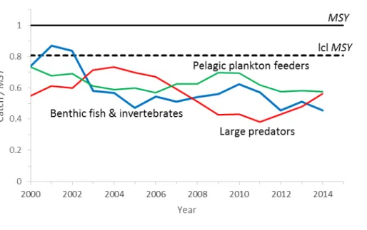
Figure 2. Catches by main functional group relative to their maximum sustainable yield (MSY, black line), for 397 stocks in the European Seas. All catches are well below the precautionary level since 2003, but are taken mostly with high effort from too small stocks (see biomass graphs below). [AllStocks_Nov09_16b.xlsx]
14
Figure 3. Cumulative total biomass of 397 stocks in the European Seas relative to the biomass that can produce the maximum sustainable yield (Bmsy = black line). The upper 95% confidence limit of Bmsy (dashed line) would present a precautionary target biomass above Bmsy. This is also the area where the maximum economic yield could be obtained. The functional groups of large predators (red), pelagic plankton feeders (green), and benthic organisms (blue) are indicated. Summed biomass of large predators has increased in recent years. [AllStocks_Nov09_16b.xlsx]
Figure 4. Median biomass relative to the level that can produce the maximum sustainable yield (B/Bmsy) for 397 stocks in the European Seas assigned to main functional groups. Note that median biomass of large predators has not increased, in contrast to the summed biomass across all stocks. This suggests that the increase stems only from few stocks.
[AllStocks_Nov09_16b.xlsx]
0 10 20 30 40 50 60 70 80 90
2000 2002 2004 2006 2008 2010 2012 2014
Biomass (million tonnes) Bmsy
Benthic fish & invertebrates Pelagic plankton feeders
Large predators
ucl Bmsy
15
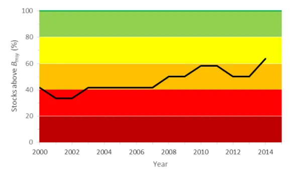
Figure 5. Percentage of stocks where biomass is above the level that can produce the maximum sustainable yield (Bmsy) for 397 stocks in the European Seas (black curve). The colors indicate visually the compliance with the goals of the Common Fisheries Policy, where all stocks (100%) shall be above Bmsy eventually. In 2014, only 16% of the stocks fulfilled that requirement.
[AllStocks_Nov09_16b.xlsx]
Figure 6. Percentage of stocks where fishing mortality F is at or below the level that can produce the maximum sustainable yield (Fmsy) for 397 stocks in the European Seas (black curve). The colors indicate visually the compliance with the goals of the Common Fisheries Policy, where all stocks (100%) shall be at or below Fmsy in 2015, latest in 2020. In 2014, only 34% of the stocks fulfilled that requirement. [AllStocks_Nov09_16b.xlsx]
16
Figure 7. Median fishing pressure relative to the maximum sustainable level (F/Fmsy) for 397 stocks in the European Seas assigned to main functional groups. Median fishing pressure is above the maximum sustainable level in all groups, with plankton feeders showing a decreasing trend in recent years. [AllStocks_Nov09_16b.xlsx]
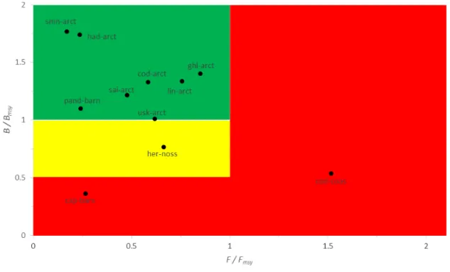
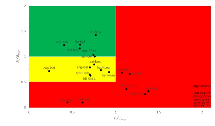
Figure 8. Presentation of 397 stocks in European Seas in a pressure (F/Fmsy) – state (B/Bmsy) plot. The red area indicates stocks that are being overfished or are outside of safe biological limits. The yellow area indicates recovering stocks. The green area indicates stocks subject to sustainable fishing pressure and of a healthy stock size that can produce high yields close to MSY.
Several stocks are not shown because their fishing pressure was beyond the upper end of the X-axis. Note that several depleted stocks are not recovering despite zero commercial catches (lower left corner). [AllStocks_Nov09_16b.xlsx]
17
The results are summarized by ecoregion in Table 3. The number of stocks with available data in an ecoregion ranges from 7 in the Black Sea to 47 in the Celtic Seas. Barents Sea and Norwegian Sea have the highest percentage (50%) of stocks that comply with the goals of the Common Fisheries Policy (CFP 2013) by having a biomass above the level that can produce MSY and being subject to sustainable exploitation.
Biomass and catches are also highest in this ecoregion, followed by wide-ranging stocks and by the Greater North Sea. The Mediterranean and Black Sea are still far away from the goals of the CFP, with only 2 out of 176 stocks in compliance.
Biomass in the ecoregions of the Mediterranean and Black Sea was on average less than half (44%) of the level that can produce MSY, whereas in the northern ecoregions (Barents Sea to Iberian Sea) biomass was about ¾ (73%) of that level. Consequently, rebuilding of biomass above the MSY level will require only 1- 6 years in many stocks in the northern region, depending on the depletion level of the stocks and how far F is reduced below Fmsy during the rebuilding phase. For example, F = 0.5 Fmsy should lead to rebuilding in 1-5 years in most stocks. In contrast, rebuilding in the Mediterranean and Black Sea may take 1-7 years under similar conditions. Note that with F = Fmsy no rebuilding above MSY levels is possible because with such fishing pressure, by definition, Bmsy is approached asymptotically in infinite time.
Detailed assessments by ecoregion are given in the next chapter.
18
Table 3. Stock numbers, stocks subject to sustainable exploitation (F <= Fmsy), stock size above the level capable of producing MSY (B > Bmsy), stocks outside of safe biological limits (B < 0.5 Bmsy), severely depleted stocks (B < 0.2 Bmsy), number and percentage of stocks that are sustainably exploited (F <= Fmsy, catch < MSY, B > 0.2 Bmsy), total biomass, total biomass level capable of producing MSY, total catch, total MSY level, and compliance with CFP targets, for 397 stocks in 14 European ecoregions and two wide-ranging regions.
Note that totals of columns in this table may be different from totals mentioned in the text because of rounding. [AllStocks_Nov09_16b.xlsx]
Ecoregion Stocks
n F <=
Fmsy n (%)
B >
Bmsy
n (%)
B < 0.5 Bmsy n (%)
B < 0.2 Bmsy n (%)
Sustainable
n (%) Biomass million tonnes
Bmsy
million tonnes
Catch million tonnes
million MSY tonnes
conform CFP n (%) Barents Sea and
Norwegian Sea 12 10 (83) 8 (67) 2 (17) 1 (8) 8 (67) 19 21 1.9 4.6 6 (50)
Iceland, Faroes
and Greenland 26 15 (58) 5 (23) 11 (42) 5 (19) 12 (50) 3.7 6.8 0.6 1.6 4 (15) Greater North Sea 45 25 (56) 9 (20) 21 (47) 6 (13) 23 (51) 9.9 11 1.6 3.4 9 (20)
Baltic Sea 20 12 (60) 6 (30) 9 (45) 1 (5) 12 (60) 3.1 4.0 0.69 0.96 5 (25)
Celtic Seas and
Rockall 47 25 (53) 11 (23) 19 (40) 7 (15) 22 (47) 1.3 2.1 0.23 0.48 10 (21)
Bay of Biscay, Iberian Coast and Azores
31 13 (42) 5 (16) 7 (23) 3 (10) 12 (39) 0.86 1.3 0.20 0.34 4 (13)
Gulf of Lions 15 2 (13) 0 (0) 13 (87) 0 (0) 2 (13) 0.044 0.11 0.009 0.033 0 (0)
Balearic Sea 22 1 (5) 0 (0) 14 (64) 0 (0) 1 (5) 0.36 0.72 0.13 0.21 0 (0)
Sardinia 19 1 (5) 0 (0) 13 (68) 4 (21) 0 (0) 0.075 0.17 0.015 0.057 0 (0)
Adriatic Sea 30 11 (37) 4 (13) 20 (67) 4 (13) 7 (23) 0.41 0.77 0.14 0.19 1 (3) Ionian Sea 31 5 (16) 0 (0) 19 (61) 4 (13) 5 (16) 0.14 0.36 0.046 0.099 0 (0)
Aegean Sea 42 5 (12) 0 (0) 23 (55) 3 (7) 5 (12) 0.19 0.38 0.070 0.112 0 (0)
Cyprus 10 0 (0) 0 (0) 9 (90) 1 (10) 0 (0) 0.0013 0.0052 0.00037 0.0015 0 (0)
Black Sea 7 1 (14) 1 (14) 3 (43) 2 (29) 1 (14) 0.68 1.3 0.24 0.40 1 (14)
Wide-ranging
ICCAT 10 5 (50) 5 (50) 1 (10) 1 (10) 5 (50) 1.0 0.96 0.13 0.19 4 (40)
Wide-ranging ICES 30 13 (43) 5 (17) 18 (60) 8 (27) 8 (27) 10.6 11.9 2.8 2.7 2 (7)
19
Comparison of independent F/Fmsy estimates with those obtained in this study
Out of the 397 stocks examined in this study, 93 (23%) had independent stock assessment estimates of Fmsy and F in in the final year with available data (Table 4). A comparison with the estimates derived in this study shows that 62 (67%) were less than 50% different from the independent stock assessment estimates. More importantly, in 76 stocks (82%) the F/Fmsy estimates derived in this study came to the same classification of overfishing (F larger than Fmsy) than the independent estimates. In 14 of the 17 diverging cases (82%), the independent stock assessments diagnosed overfishing while this study proposed sustainable exploitation levels. These differences often occurred in severely depleted stocks, where the surplus production models applied in this study slightly overestimated final biomass and thus underestimated exploitation. Also, the independent assessments often used the fishing mortality of higher age groups to determine the F/Fmsy ratio, whereas surplus production models do not know about age structure and instead derive the F/Fmsy ratio across all age groups, weighted by their contribution to the catch. Since lower age groups are not yet fully selected by the gear, their fishing mortality is lower than that of higher age groups, and hence the F/Fmsy ratio estimated by surplus production models may be lower than that of age-structured assessments. In summary, with regard to exploitation there is good agreement between the estimates done in this study and the estimates derived by independent stock assessment groups, with the caveat that the F/Fmsy estimates in this study may underestimate the exploitation of severely depleted stocks or of stocks with many age classes.
Table 4. Comparison of exploitation estimates obtained in this study with 93 estimates in independent stock assessment documents. See respective Appendix for the ecoregion for indication of sources. Cases where estimates from this study deviate more than 50% from the “official” estimates are marked in bold in the F/Fmsy cur column. Cases where the independent classification of overfishing is different from this study are marked bold in the F/Fmsy indep column.
Region Species Stock F/Fmsy
cur F/Fmsy indep Barents Sea and Norwegian Sea Gadus morhua cod-arct 0.58 0.96
Melanogrammus
aeglefinus had-arct 0.24 0.59
Clupea harengus her-noss 0.66 0.73
Iceland, Faroes and Greenland Argentina silus arg-icel 0.70 0.77
Molva molva lin-icel 0.59 1.17
Sebastes norvegicus smr-5614 0.74 0.99
Brosme brosme usk-icel 0.58 1.1
Gadus morhua cod-farp 1.38 1.44
Melanogrammus
aeglefinus had-faro 1.34 1.02
Pollachius virens sai-faro 0.75 0.84
Clupea harengus her-vasu 0.92 1.0
Greater North Sea Solea solea sol-eche 0.81 1.73
sol-kask 0.30 0.49 sol-nsea 0.69 1.01
Gadus morhua cod-347d 0.30 1.17
Melanogrammus
aeglefinus had-346a 2.11 0.65
20
Region Species Stock F/Fmsy
cur F/Fmsy indep
Greater North Sea Merlangius merlangus whg-47d 1.18 1.51
Clupea harengus her-47d3 0.43 0.73
Sprattus sprattus spr-nsea 0.75 1.81
Baltic Sea Gadus morhua cod-2224 1.67 3.37
Clupea harengus her-2532-gor 0.82 0.83
her-30 1.05 0.97
her-3a22 0.63 0.80 her-riga 1.14 1.32
Sprattus sprattus spr-2232 1.29 1.03
Celtic Seas and Rockall Molva dypterygia bli-5b67 0.31 0.28 Lepidorhombus
whiffiagonis mgw-78 0.57 1.13
Pleuronectes platessa ple-7h-k 4.95 4.44 ple-echw 0.44 0.62 ple-iris 0.21 0.55
Solea solea sol-7h-k 0.55 2.88
sol-celt 3.70 1.13 sol-echw 0.70 0.68 sol-iris 0.63 0.38
Gadus morhua cod-7e-k 1.35 1.51
cod-iris 0.14 2.91 cod-scow 8.16 4.69 Melanogrammus
aeglefinus had-7b-k 0.88 1.30
had-rock 1.47 1.07 Merlangius merlangus whg-7e-k 0.62 0.73 whg-scow 0.91 0.32
Clupea harengus her-67bc 0.36 0.44
her-irls 0.65 0.73 her-nirs 0.63 1.01 Bay of Biscay and Iberian Sea,
including Azores Lophius piscatorius anp-8c9a 0.24 0.68
Lepidorhombus boscii mgb-8c9a 0.98 2.14 Lepidorhombus
whiffiagonis mgw-8c9a 1.28 1.38
Solea solea sol-bisc 1.05 1.34
Merluccius merluccius hke-soth 0.77 2.10 Trachurus trachurus hom-soth 0.78 0.40
Gulf of Lions Merluccius merluccius MERLMER_LI 2.54 14.9
Engraulis encrasicolus ENGRENC_LI 0.53 0.21
Balearic Sea Aristeus antennatus ARITANT_BA 1.71 4.2
Mullus barbatus MULLBAR_BA 1.48 2.78 Mullus surmuletus MULLSUR_BA 2.16 0.63 Nephrops norvegicus NEPRNOR_BA 1.23 3.46
21
Region Species Stock F/Fmsy
cur F/Fmsy indep Balearic Sea Parapenaeus longirostris PAPELON_BA 3.38 3.06
Merluccius merluccius MERLMER_BA 4.79 7.47 Micromesistius poutassou MICMPOU_BA 2.12 3.28 Engraulis encrasicolus ENGRENC_BA 1.20 2.54
Sardinia Mullus barbatus MULLBAR_SA 2.33 3.19
Nephrops norvegicus NEPRNOR_SA 2.50 1.38 Pagellus erythrinus PAGEERY_SA 2.59 2.38 Parapenaeus longirostris PAPELON_SA 1.32 1.06 Merluccius merluccius MERLMER_SA 1.66 7 Micromesistius poutassou MICMPOU_SA 1.62 2.11 Engraulis encrasicolus ENGRENC_SA 1.69 2.6
Adriatic Sea Mullus barbatus Mull_bar_AD 1.68 1.32
Solea solea Sole_sol_AD 2.06 1.42
Squilla mantis Squi_man_AD 1.09 1.23 Merluccius merluccius Merl_mer_AD 4.05 5.56 Engraulis encrasicolus Engr_enc_AD 1.31 2.9 Sardina pilchardus Sard_pil_AD 1.58 1.47
Ionian Sea Aristeomorpha foliacea ARISFOL_IS 1.67 2.28
Mullus barbatus MULLBAR_IS 3.48 2.2
Ionian Sea Parapeneaus longirostris PARELON_IS 0.91 1.63
Merluccius merluccius MERLMER_IS 3.24 4.83 Mullus barbatus MULLBAR_AL 1.97 1.08 Nephrops norvegicus NEPRNOR_AL 4.01 2.67
Cyprus Mullus barbatus MULLBAR_CY 1.53 2.09
Mullus surmuletus MULLSUR_CY 2.19 2.13
Boops boops BOOPBOO_CY 2.00 1.54
Spicara smaris SPICSMA_CY 1.59 1.54
Black Sea Mullus barbatus barbatus RMullet_BS 2.19 1.67
Squalus acanthias PDogfish_BS 1.51 3.0 Scophthalmus maximus Tur_BS 5.31 5.38 Merlangius merlangus Whiting_BS 1.49 1.37
Sprattus sprattus Spr_BS 0.83 0.95
Trachurus mediterraneus MHMackerel_BS 7.57 5.56 Engraulis encrasicolus BS_anch 1.23 2.65 Wide-ranging ICES Stocks Merluccius merluccius hke-nrtn 1.12 0.79 Micromesistius poutassou whb-comb 0.77 1.43
Scomber scombrus mac-nea 1.70 1.54
22 Results by ecoregion
Northeast Atlantic
Barents Sea and Norwegian Sea
The following paragraph describing the Barents Sea was taken from the ICES Advice 2016, Book 9, http://www.ices.dk/sites/pub/Publication%20Reports/Advice/2016/2016/Barents_Sea_Ecoregion- Ecosystem_overview.pdf.
“The Barents Sea is one of the shelf seas surrounding the Polar basin. It connects with the deeper Norwegian Sea to the west, the Arctic Ocean to the north, and the Kara Sea to the east, and borders the Norwegian and Russian coasts to the south. The 500 m depth contour is used to delineate the continental slope to the west and the north. To the east the Novaya Zemlya archipelago separates the Barents Sea and the Kara Sea. The Barents Sea covers an area of approximately 1.6 million km2, has an average depth of ca. 230 m, and a maximum depth of about 500 m at the western end of Bear Island Trough. Its topography is characterized by troughs and basins, separated by shallow bank areas. The three largest banks are Central Bank, Great Bank, and Spitsbergen Bank. Several troughs over 300 m deep run from the central Barents Sea to the northern (e.g. Franz Victoria Trough) and western (e.g. Bear Island Trough) continental shelf break. These western troughs allow influx of Atlantic waters to the central Barents Sea.
Atlantic waters enter the Arctic Basin through the Barents Sea and the Fram Strait. Large-scale atmospheric pressure systems influence the volume flux, temperature, and salinity of Atlantic waters, in turn affecting oceanographic conditions both in the Barents Sea and in the Arctic Ocean.”
Figure 9. The Barents Sea ecoregion with EEZ delineations. Source: ICES Advice 2016, Book 9.
23
The following paragraph describing the Norwegian Sea was taken from the ICES Advice 2009, Book 3, http://www.ices.dk/sites/pub/Publication%20Reports/ICES%20Advice/2009/ICES%20ADVICE%202009%
20Book%203.pdf.
“The Norwegian Sea is traditionally defined as the ocean bounded by a line drawn from the Norwegian Coast at about 62°N to Shetland, farther to the Faroes-East Iceland-Jan Mayen-the southern tip of Spitsbergen-the Vesterålen at the Norwegian coast and the along the coast. In addition a wedge shaped strip along the western coast of Spitsbergen is included. The offshore boundaries follow in large part the mid Atlantic subsurface ridges. The Norwegian Sea has an area of 1.1 million km2 and a volume of more than 2 million km3, i.e. an average depth of about 2000 m. The Norwegian Sea is divided into two separate basins (the Lofoten Basin to the south and the Norwegian Basin in the north) of 3000 m to 4000 m depth, with a maximum depth 4020 m. Along the Norwegian coast there is a relatively narrow continental shelf, between 40 and 200 km wide with varied topography and geology. It has a relatively level sea bottom with depths between 100 and 400 m. The shelf is crossed by several troughs deeper than 300. Moraine deposits dominate the bottom substratum on the shelf, but soft layered clay is commonly found in the deeper parts. Gravelly and sandy bottoms are found near the shelf break and on ridges where the currents are strong and the sedimentation rates low.”
ICES assessment reports with data until 2015 were analyzed for 12 stocks in the Barents Sea and Norwegian Sea. The graphs below summarize their status and exploitation level within an MSY- framework. The list of species and their current exploitation and status is summarized in Table 5. Detailed assessments for every stock are available in Appendix 1 and in the spreadsheet BarentsSea_Sep26_2016.xlsx.
Of the 12 stocks, 2 (17%) were subject to ongoing overfishing (F > Fmsy) and 2 stocks (17%) were outside of safe biological limits (B < 0.5 Bmsy). In two stocks (17%) catches exceeded the maximum sustainable yield (C/MSY > 1). One stock of redfish (smr-arct) was in critical condition, defined by being outside of safe biological limits and subject to overfishing (marked red in Table 5). Altogether, 4 stocks (33%) were subject to unsustainable exploitation (catch > MSY or F > Fmsy or B < 0.2 Bmsy), with the too high catches marked red in Table 5. Six stocks (50%) could be considered as being well managed and in good condition sensu CFP (2013), defined by not being subject to overfishing (F > Fmsy or Catch > MSY) and having a biomass above the one that can produce the maximum sustainable yield.
Summed biomass of the 12 stocks of 19 million tonnes in the last year with available data was below but close to the biomass level of 21 million tonnes that can produce maximum yields. Summed catches of 1.9 million tonnes were well below the summed maximum sustainable yield of 4.6 million tonnes. Because of trophic interactions it is not possible to achieve MSY simultaneously for all stocks, but sustained catches of near the lower confidence limit or near 90% of MSY (whichever is lower) would be possible if all stocks have recovered above Bmsy. Because of more fish in the water, such catches could be obtained with much less fishing effort and much less impact on the ecosystem. See legends of Figures for more comments.
24
Table 5. Analysis of 12 stocks in the Barents Sea and Norwegian Sea, with indication of last year with available data (Year), maximum sustainable yield (MSY), absolute and relative catch (Catch, C/MSY), maximum sustainable fishing mortality (Fmsy) if the stock is within safe biological limits (B/Bmsy > 0.5), Fmsy for current stock size, F/Fmsy for current stock size, biomass that can produce MSY (Bmsy), relative biomass (B/Bmsy). Scientific names of healthy stocks where F/Fmsy < 1 and B/Bmsy > 1 are marked green and stocks outside of safe biological limits (B/Bmsy < 0.5) with ongoing overfishing (F/Fmsy > 1) are marked red. Catches above MSY are marked bold (C/MSY > 1). Overfishing with F/Fmsy > 1 is marked bold. Stock sizes outside safe biological limits (B/Bmsy < 0.5) are marked bold. Unsustainable catches (catch > MSY, F > Fmsy, B < 0.2 Bmsy) are marked red. Catches are given in tonnes per year. Biomass is given in tonnes as average total biomass during the year. Species are sorted by functional groups as indicated by the color of the stock IDs:
benthic fish & invertebrates (blue), large predators (red) and pelagic plankton feeders (green). [BarentsSea_Sep26_2016.xlsx]
Scientific name Stock Year MSY Catch C/MSY Fmsy Fmsy cur
F F/Fmsy cur
Bmsy B B/Bmsy
Reinhardtius
hippoglossoides ghl-arct 2014 18,674 22,244 1.19 0.19 0.19 0.16 0.85 97,494 136,757 1.40 Molva molva lin-arct 2014 9,516 9,606 1.01 0.16 0.16 0.12 0.76 58,857 78,612 1.34 Pandalus borealis pand-
barn 2014 62,740 16,671 0.27 0.37 0.37 0.09 0.24 168,188 185,115 1.10 Sebastes mentella smn-arct 2013 30,923 9,297 0.30 0.25 0.25 0.04 0.17 123,181 217,555 1.77 Sebastes norvegicus smr-arct 2015 18,619 3,630 0.19 0.15 0.03 0.29 9.37 124,272 12,678 0.10 Brosme brosme usk-arct 2014 13,965 8,734 0.63 0.28 0.28 0.17 0.62 50,642 51,223 1.01 Gadus morhua cod-arct 2015 1,116,189 864,384 0.77 0.23 0.23 0.13 0.58 4,857,246 6,451,009 1.33 Gadus morhua cod-coas 2015 64,205 52,154 0.81 0.28 0.28 0.43 1.52 226,986 121,657 0.54 Melanogrammus
aeglefinus had-arct 2015 474,993 194,756 0.41 0.21 0.21 0.05 0.24 2,311,421 4,020,476 1.74 Pollachius virens sai-arct 2015 227,311 131,765 0.58 0.27 0.27 0.13 0.48 849,200 1,032,863 1.22 Mallotus villosus cap-bars 2015 1,670,405 115,000 0.07 0.21 0.15 0.04 0.26 8,098,440 2,920,786 0.36 Clupea harengus her-noss 2014 905,483 461,306 0.51 0.20 0.20 0.13 0.66 4,487,167 3,442,750 0.77
25
Figure 10. Cumulative catches for 12 stocks in the Barents Sea and Norwegian Sea, with indication of main functional groups.
The black line indicates the maximum sustainable yield (MSY) for the ecoregion and the dashed line indicates the lower 95%
confidence limit as a precautionary target. [BarentsSea_Sep26_2016.xlsx]
Figure 11. Catches by main functional group relative to their maximum sustainable yield (MSY, black line), for 12 stocks in the Barents Sea and Norwegian Sea. Catches for large predators (red curve) are near the precautionary maximum. Catches for pelagic plankton feeders (green curve) can be increased after the stocks have been rebuilt. [BarentsSea_Sep26_2016.xlsx]