GEOLOGICAL SURVEY OF CANADA OPEN FILE 8008
Assessment of submarine slope failures off Vancouver Island, British Columbia
M. Riedel, K. Naegeli, M.M. Côté
2016
GEOLOGICAL SURVEY OF CANADA OPEN FILE 8008
Assessment of submarine slope failures off Vancouver Island, British Columbia
M. Riedel1*, K. Naegeli2, M.M. Côté1
1 Natural Resources Canada, Geological Survey of Canada, 9860 West Saanich Road, Sidney, British Columbia
2University Fribourg, Department of Geosciences, Fribourg, CH-1700, Switzerland
*Current address: GEOMAR Helmholtz Centre for Ocean Research Kiel, 24148 Kiel, Germany
2016
© Her Majesty the Queen in Right of Canada, as represented by the Minister of Natural Resources, 2016
Information contained in this publication or product may be reproduced, in part or in whole, and by any means, for personal or public non-commercial purposes, without charge or further permission, unless otherwise specified.
You are asked to:
• exercise due diligence in ensuring the accuracy of the materials reproduced;
• indicate the complete title of the materials reproduced, and the name of the author organization; and
• indicate that the reproduction is a copy of an official work that is published by Natural Resources Canada (NRCan) and that the reproduction has not been produced in affiliation with, or with the endorsement of, NRCan.
Commercial reproduction and distribution is prohibited except with written permission from NRCan. For more information, contact NRCan at nrcan.copyrightdroitdauteur.rncan@canada.ca.
doi:10.4095/297904
This publication is available for free download through GEOSCAN (http://geoscan.nrcan.gc.ca/).
Recommended citation
Riedel, M., Naegeli, K., and Côté, M.M., 2016. Assessment of submarine slope failures off Vancouver Island, British Columbia; Geological Survey of Canada, Open File 8008, 108 p. doi:10.4095/297904
Publications in this series have not been edited; they are released as submitted by the author.
1 Table of contents
Abstract …2
1 Introduction …3
2 Geological Background …4
3 Data and Methods …6
4 Results …7 5 Discussion ...61
6 Conclusions ...72
7 References ...73
Appendix ...78
2 Abstract
Multibeam bathymetric data acquired off Vancouver Island across the accretionary prism of the Cascadia subduction zone reveal a prominent segmentation of the deformation front with dominant azimuths of the ridges at ~120° and ~150° and abundant submarine landslides. Both these ridge-orientations are oblique to the direction of subduction (~45°).
Ridges at a strike of ~120° show dominantly rectangular-shaped failure head-scarps and intact blocks of sediments within the failed sediment mass, whereas ridges with an azimuth of ~150° show curved head-scarps and incoherent debris in the failure mass. We propose that this systematic change in failure-style is related to the underlying thrust fault system producing steeper and taller ridges for azimuths around 150°, but less steep and tall ridges at 120°. Thus, debris-flow style failure is simply a result of higher kinetic forcing of the down-sliding sediment mass: more mixing and destruction of the coherent blocks for taller and steeper ridges, and blocks of intact sediment for gentle slopes and less elevated ridges. A segmentation of the deformation front and ridge alignment into two dominant azimuths could be a result of: a) complex interaction and competing forces from overall slab-pull (45°), b) re-activated faults orientated almost N-S (~175°) on the oceanic plate and overlying sediment cover (reflected in the magnetic stripes and abyssal plain strike-slip faulting), and c) relative orientation of the back-stop off Vancouver Island and accreted terranes (at ~127° following the coastline between Nootka Island and Port Renfrew). Extensional faulting is observed only at ridges with debris-flow style failure, which also are the ridges with larger height and steeper slopes. These extensional faults may be the result of over-steepening of the ridges and collapse of the sediment pile that can no longer withstand its own weight due to limited internal shear strength.
3 1 Introduction
The convergent margin of the Cascadia subduction zone off Vancouver Island has experienced repeat megathrust earthquakes with magnitudes M>8 and associated tsunamis (e.g. Rogers, 1988; Hyndman and Rogers, 2010). Estimates of the hazard and earthquake risk, disaster mitigation and management in the affected region of British Columbia are continuously assessed and updated (e.g. Adams and Halchuk, 2003; Onur and Seeman, 2004; Levson et al., 2003; Monahan et al., 2000; Canada's Platform for Disaster Risk Reduction, 2013).
Historic evidence for large earthquakes in this region was first documented by Atwater (1987) using sedimentary records of deep-water turbidites. The date of the last megathrust event was determined by Satake et al. (1996) to be January 26, 1700, using tsunami records in Japan. The recurrence rate of such events off Cascadia varies between 250 and~1000 years (Goldfinger et al., 2012).A series of frontal ridges of the northern Cascadia convergent margin (Fig. 1) was investigated during research expedition2008007PGC in August 2008 aboard the Canadian Coast Guard Ship (CCGS) John P. Tully (Haacke et al., 2008). The purpose of the expedition was to characterize the sediments hosting gas hydrate deposits and to assess the role of gas hydrates in altering sediment properties and possibly affecting the nature of submarine slope failures potentially triggered by megathrust earthquakes and their tsunami potential (later further assessed by Scholz, 2013). The most striking outcome of the cores taken at the frontal ridges was a detailed record of turbidite events allowing the reconstruction of past megathrust earthquakes off Vancouver Island (Hamilton et al., 2015).
Here we report on the general nature of the slope failures, assess the geographical constraints of the frontal ridges, and show linkages between style of failure and ridge- morphology and physiography. A simple model is presented explaining the style of slope failure as a result of slide kinematics driven by ridge height and slope-angle. However, geographical distribution and alignment of the frontal ridges in dominant orientations along the margin remain enigmatic.
4 2 Geological background
The Cascadia subduction zone extends from Cape Mendocino, California, to the northern end of Vancouver Island, British Columbia. The Juan de Fuca plate is subducting beneath the North American plate at a rate of ~45 mm/yr (e.g. Riddihough, 1984). Offshore of Vancouver Island the oceanic plate is relatively young (2 to 6 Ma), and therefore warm and buoyant (Davis et al., 1990). The 1 km to 2 km-thick sedimentary section that lies on top of the oceanic plate near the deformation front consists of a mix of fine-grained hemi-pelagic sediments and coarser-grained turbidites (e.g. Westbrook et al., 1994). At the deformation front, the sedimentary section is mainly scraped off and accreted to the margin (e.g. Davis and Hyndman, 1989). As a result, the accretionary prism consists of a series of ridges and folds (Fig. 1). The accretion of sediments is accompanied by overall sediment thickening and deformation, bulk shortening, as well as fluid expulsion (e.g. Hyndman et al., 1993). The upwardly expelled fluids are rich in methane, and as a consequence, gas hydrate occurs across the prism from the deformation front to the eastward limit of gas hydrate stability in water depths of ~900 m (e.g. Riedel et al., 2010). Several boreholes have been drilled off Vancouver Island during Ocean Drilling Program (ODP) Leg 146 and Integrated Ocean Drilling Program (IODP) Expedition 311, which document the gas hydrate environment and associated sedimentology (e.g. Westbrook et al., 1994; Riedel et al., 2006).
5 Figure 1 Bathymetric EM300 multibeam data with location of slope failures discussed in this report. Locations of semi-circular depressions are shown by grey arrows. Inset shows study region off Vancouver Island and the extent of the NEPTUNE cable. [O.B. = Field of out-runner blocks]
6 3 Data and Methodology
Two types of data are available for the analyses of the slope failures off Vancouver Island. Legacy data from early seafloor mapping of the margin with the SEAMARK II system (Davis et al., 1987; Davis and Hyndman, 1989) provide backscatter imagery of the seafloor. These data were digitized from paper-records and converted to geo-referenced images for use within ArcGIS®. Modern seafloor multibeam data were acquired in 2002 with the EM300 system on the R/V Thompson from the University of Washington. The data are available in a 20×20 m grid (first-pass processing with acquisition footprint not removed), and a lower-resolution 40×40 m grid of data with noise from far-angle beams removed (Fig.2). Overall, the high resolution grid of the multibeam data is preferred over the coarser data as it is much sharper and allows a better definition of physical features, despite the acquisition footprint being visible, and potentially compromising accuracy of results in e.g. the definition of failure volume.
The high-resolution bathymetric data were used to derive statistical parameters of seafloor shape (azimuth, width, height, slope-angle of ridges, failure-volume). First, an image of the bathymetry data was exported at a scale of 1:250,000 and imported into an image processing tool. Individual lineaments were identified and digitized on the bathymetry image and then converted to ridge-length and azimuth (see section 4). To augment this subjective analysis, an objective measure of azimuth (strike) for the slope- failure regions from the bathymetric data was calculated. Using ArcGIS®, the aspect (direction of slope) was determined from the bathymetric data, from which the azimuth is calculated by adding 90°. Around the individual failures, ridge azimuths were defined by extracting the aspect values over a selected region, and then imported as histogram into MATLAB® to perform a Gaussian polynomial fit. Orientation-ambiguity from symmetry around 360° and 180° was removed prior to defining the average azimuth. The maximum value returned from the best-fit Gaussian function is used in all additional calculations and discussions.
Individual profiles were generated perpendicular and parallel to the major ridges with slope failures, from which minimum, maximum, and average slope angles for the ridge and failure plane were derived, as well as height and width of the ridges.
7 To estimate slope failure volumes, first we reconstructed the ridge before the failure happened, using the high-resolution bathymetric data. Therefore we generated a virtual plane covering the landslide in a shape resembling that of the adjacent intact portions of the frontal ridges. The area of the slope failure was defined only from the bathymetry data. The difference in the multibeam bathymetry data and the virtual plane defines the failure volume and zones of net-loss and net-gain were defined in the region of the exposed failure plain. We did not measure the volume of debris in front of some of the slope-failures to compare it to the volume estimates as described above, due to the lack of sub-bottom profiler data defining the sole of the failure-mass that may have eroded portion of the original seafloor. Therefore, these volume estimates are only approximate, but can be used as first guide to estimate any tsunami potential.
Borehole data from IODP Expedition 311 are used to define the stress-regime of the upper-most 300 m of sediments across the prism. Borehole breakouts have previously been used successfully to define such stress orientation of Southern Hydrate Ridge off Oregon (Goldberg and Janik, 2006). The electrical resistivity measured during logging- while-drilling (LWD) directly above the drill bit (referred to as resistivity at bit, or RAB) produces a 360° image of the borehole wall. Due to horizontal stresses, the borehole is not circular but is deformed resulting in a cylindrical shape of the hole. Thus, low- resistivity stripes can be seen in the RAB-image, where the LWD-tool has a poorer contact to the borehole wall. The maximum horizontal stress that squeezes the borehole is oriented perpendicular to that defined by the low-resistivity striping. These orientations from all five sites of IODP Expedition 311 were then superimposed on the strike- orientations of the bathymetric data to investigate linkages between the stress regime and the surface expressions of sediment accretion.
8 Figure 2 Comparison of bathymetric data fidelity of the (a) 20×20 m grid with acquisition footprint, and (b) a re-processed, lower resolution 40×40 m grid.
9 4 Results
We identified 13 major slope failures and one field of out-runner blocks, along the frontal ridges of the accretionary prism of the Juan de Fuca Plate over a distance of 175 km (Fig. 1). For the purpose of this report, these failures are labelled alphabetically A to M, from south to north.
The slope failures show two different types: 1) rectangular head-scarps, often associated with intact sediment blocks in the failed mass, or 2) curved head-scarps and the failed sediments often appear as an incoherent mass (referred to as ‘debris flow’). All failures were identified from the seafloor bathymetry by their apparent “fresh” look, with visible head-scarp, exposed failure plain, and sedimentary material deposited down-slope that are not covered by recent sediments. Numerous additional slope-failures that are apparently older and are covered by a sediment drape are also identified, but are not analysed in this study.
4.1 General margin-wide observations
The bathymetric data show a pattern of individual small ridges along the deformation front. Individual ridges do not occur as a single (intact) ridge, but rather are broken into short (5-12 km) segments at distinctly different azimuths. In order to define the strike orientation of the various ridges, the bathymetry data were manually digitized by drawing lineaments across ridges and scarps (Fig. 3). Using these lineaments, the azimuths and scale-length were defined (Fig. 4). Two dominant azimuths of ~110° and 150° are identified in the rose-diagram (Fig. 4). A polar plot of the length of ridges and their azimuths is presented in Figure 5. Ridge length is mostly below 7 km with few longer lineaments up to 12.5 km. No correlation between length and azimuth of all lineaments can be seen.
Borehole breakouts were defined from the RAB resistivity data of the borehole wall (Fig. 6). Average orientations of the breakouts are generated as well as minimum and maximum angles from the overall width of the breakouts. The orientations are then superimposed in Figure 3 in form of the direction of maximum compression. A rotation by 90° was then applied to represent strike orientation as shown in Figure 4.
10 Breakouts are not uniformly distributed over the entire depth-range drilled at the four sites (Fig. 6). Breakouts at Site U1326 are diffuse and occur from depths as shallow as 20 mbsf down to 300 mbsf. At Site U1325 breakouts are most obvious at depths below 250 mbsf, but can be traced as shallow as ~100 mbsf. Site U1327, at the central slope, is dominated by a massive gas hydrate lens at 120-145 mbsf but breakouts appear from ~25 mbsf to the bottom of the hole. The cold vent site U1328 has massive fracture- dominated gas hydrate occurrences within the top 50 mbsf. A second fracture is intersected at ~95 mbsf but breakouts appear across the entire depth range penetrated.
Site U1329, at the eastern edge of the drilling transect shows breakouts starting at depths of ~70 mbsf. These breakouts seem to be less dominant in the lower section of the borehole, where an unconformity was penetrated at ~125 mbsf and much higher electrical resistivity was measured in these highly compacted and low-porosity sediments.
The orientation of the breakouts at four sites is almost identical and lies between 25° and 35°. Maximum compression appears to be in the orientation of ridges with azimuths around 120°. The exception is Site U1325 at the basin just east of the frontal ridge, where the breakouts suggest an orientation of maximum compression that is orientated at 95°-100°.
11
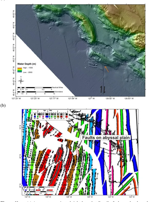
12 Figure 3 (a) Map showing northern portion of the data coverage (up to the Nootka Fault zone) with bathymetric data. Manually-digitized lineaments are represented with dashed-lines, where black lines are part of the accretionary prism of the Juan de Fuca Plate and white lines are part of the Explorer Plate. (b) Map showing the southern portion of the data coverage with bathymetric data. Manually-digitized lineaments are represented with dashed-lines and the orientation of compression from borehole breakouts at the sites from IODP Expedition 311 are represented in dark blue. The azimuth of the vector of subduction for Cascadia off Vancouver Island is indicated by the arrow (MORVEL=Mid-Ocean Ridge Velocity, DeMets et al., 2010).
13 Figure 4 Rose diagram of the azimuths of manually-digitized lineaments as seen in Figure 3. Orientations of compression are rotated to represent strike orientation (+90°) of the MORVEL vector of the main subduction orientation (black dashed line) and borehole breakouts (dotted blue lines) are shown (see Figure 6 for details on breakouts). A distinction between lineaments from frontal ridges with rectangular head-scarps and mostly blocky failures (red) versus those from failures with curved head-scarps and debris-flows (green) is made.
14 Figure 5 Distribution of (a) azimuths and (b) lengths of all lineaments in Figure 3 and (c) composite diagram of azimuths (°) vs. lengths (m) plotted as radius.
15 Figure 6 LWD data from IODP Expedition 311 at all five sites (location see Fig. 3), shown from west (U1326) to east (U1329). Vertical green dashed lines are the average position of breakouts. Data used in Figure 4 include the range of angles defined from the width of the breakouts seen in the RAB images. The black dashed line represents the base of gas hydrate stability zone. To the left of each RAB image, the lithostratigraphic units are shown (Riedel et al., 2006). Breakouts with no change in orientation are seen across all units as well as above and below the gas hydrate stability zone, indicating a prevailing stress orientation.
16 The analysis shows two categories of failure: (1) blocky-failures with sharp, rectangular head-scarps (A, C, D, F, H, I, J, and K) and (2) debris-flow style failures with circular head-scarps (B, E, and G). An exception is seen for slope failures associated with a large (L, M), 18 km long ridge at the Nootka Fault zone, where the ridge orientation is nearly N-S. At this location, large blocks have broken off the ridge semi- intact and are seen at the foot of the ridge, whereas the head-scarps are curved. The ridge belongs to the accretionary margin of the Explorer Plate. A point of rotation with an abrupt change in ridge-orientation is seen at 49°7.7′ N, 127°39.8′ W (Fig. 3a). This marks the transition between the accretionary complexes of the Juan de Fuca and Explorer plates.
All failures within Category 1 appear along ridges with an azimuth of ~114°
(Table 1, Fig. 4), whereas the failures in Category 2 are along ridges with an azimuth of
~167° (Table 1, Fig. 4).
There is no obvious correlation between failure category and failure volume (Table 1), width or length of the failure material. However, the ridges associated with debris flow style failures (Category 2) have steep slopes (17 - 25º) and high elevation (790 – 985 m) above the abyssal plain, whereas the failures of Category 1 occur at ridges of generally less elevation (370 – 540 m) and more gentle slopes (10 - 17º).
Several of the slope failures are associated with a debris-cone that is larger in lateral extent than what is revealed by the multibeam bathymetry data. The SEAMARK- II acoustic data show these debris-cones as high backscatter regions at failures A, C, D, E, and F. The absence of high backscatter material at the foot of the ridges for the other failures may be attributed to them being slightly older and where recent pelagic sedimentation may have covered the original debris with a sufficiently thick drape to suppress the backscatter signal. However, we lack sufficient 3.5 kHz sub-bottom data coverage to support this hypothesis.
17 Table 1 Geomorphologic details of the 13 major slope failures, (ND: not defined, rect.: rectangular, curv.: curved).
Failure style
Head- scarp
Ridge height
(m)
Ridge width (km)
Failure width
(km)
Failure length
(km)
Failure area (km2)
Azimuth of ridge
(°)
Volume loss (km3)
Volume gain (km3)
Net loss (km3)
Range in failure
angle (°)
Average failure
angle (°)
Intact ridge slope angle
(°)
A Blocky rect. 470 2.0 3.3 1.3 4.1 106.2 0.471 0.019 0.452 12.5 - 29.4 18.9 14.5
B Debris curv. 985 4.95 2.5 2.2 4.6 165.0 0.773 0.013 0.760 10.6 - 24.0 18.0 25.0
C Blocky rect. 550 1.9 2.4 0.7 1.5 126.0 0.049 0.007 0.042 12.7 - 16.4 14.4 12.8
D Blocky rect. 500 3.05 3.3 2.0 5.0 109.8 0.257 0.035 0.222 8.4 - 25.7 16.1 9.5
E Debris curv. 880 4.48 2.0 2.4 2.7 150.1 0.468 0.008 0.460 12.2 - 26.8 17.3 16.5
F Blocky rect. 370 3.65 2.0 1.2 2.3 100.6 0.128 0.004 0.128 5.7 - 16.0 11.5 11.8
G Debris curv. 790 3.9 1.8 1.4 2.0 146.7 0.151 0.007 0.151 12.5 - 24.0 20.0 21.5
H Blocky rect. 540 3.0 2.0 2.0 3.2 126.3 0.019 0.019 0.000 10.2 - 15.7 13.0 11.5
I ND rect. 370 2.9 0.8 1.8 1.2 117.6 0.044 0.003 0.041 10.0 - 35.0 18.0 9.0
J Blocky rect. 450 2.7 1.9 3.4 6.5 154.5 0.339 0.007 0.332 3.0 - 35.0 14.0 10.7
K Blocky rect. 495 1.8 0.8 1.5 1.0 138.4 0.076 0.001 0.075 2.0 - 35.0 15.0 12.8
L Blocky curv. 1075 6.0 1.7 2.5 3.9 8.0 0.210 0.006 0.204 15.0 - 38.0 25.0 16.0
M Blocky curv. 1340 6.2 1.9 3.7 6.4 177.6 0.352 0.037 0.315 15.0 - 38.0 30.0 16.0
In the following sections, the detailed features of each of the slope failures are described.
18 4.2 Failure A
Slope failure A shows rectangular head-scarps (Fig. 7a). It occurs in a region which is characterized by land-ward verging thrust faults (e.g. Yuan et al., 1994). The ridge rises ~470 m above the abyssal plain (Table 1). Failure A is ~3.3 km wide and 1.3 km long with an area of ~4.1 km2 (Table 1). Data from seafloor acoustic imaging (Davis et al., 1987) reveal two high-backscatter regions around the blocky failure mass (Fig.
7b).The headwall shows a fairly straight shape and the entire ridge has an azimuth of
~106° as defined from the aspect of the bathymetric data (Fig. 8, Table 1).Profiles drawn across the failure and ridge (Fig.A-1) show a minimum slope angle of 12° (Table 1), with the steepest part of failure A having an angle of 29° (Fig. 7c).Based on our calculations, the volume of sediment loss associated with failure A is 0.47 km3 (Table 1, Fig. A-2).The intact ridge shows an average slope angle of 13°.
The western of the two high backscatter regions extends ~3 km further to the south of the blocks. The second field of high backscatter emanating from failure A is bound by the ridge located further to the west. Portions of this western-most ridge are covered by high-backscatter material. Two additional slope-failure related high backscatter regions are seen to the SE of failure A, bound by the bathymetric features of the ridge-system. These two regions have a weaker backscatter signal than that of the field associated with failure A, suggesting a greater age of these failures assuming that the failure debris is covered with a post-failure drape reducing the backscatter signal. Just north of failure A is a semi-circular depression with moderately high backscatter which is the current depo-centre of Barkley Canyon. As seen in Figure 3b, further west off this depression a series of sediment waves have developed.
19 Figure 7 (a) Multibeam bathymetry and relief, (b)
with superimposed backscatter. High-amplitude debris fields are outlined by red dashed lines. Head-scarps are shown as thin black lines. Additional high backscatter regions (green dashed line) are linked to smaller failures (black arrows). The magenta-dashed line shows the current depo-centre of Barkley Canyon; grey arrows show sediment transport pathway. Location of profiles used to define ridge symmetry and failure statistics are indicated, see Fig. A-1. (c) Map of slope angle.
20 Figure 8 (a) Map of regional aspect derived from bathymetry and (b) distribution of azimuth values over selected polygonal region (black dashed line). The polygon was selected to avoid the slope failure. A best-fit 1-term Gaussian polynomial fit yields an average azimuth of 106.2° (Table 1). The azimuth values (calculated from aspect) were used for a higher degree of symmetry of the Gaussian function and thus optimized best-fit analysis.
21 4.3 Failure B
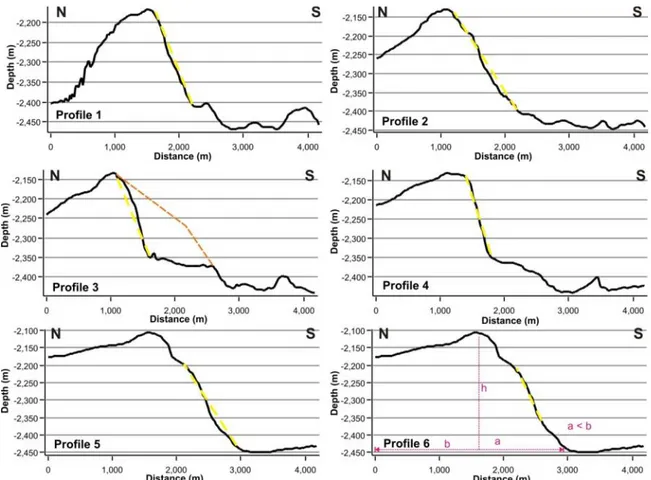
Failure B is a debris-flow style failure (Fig. 9a) with a curved head-scarp. The ridge rises ~985 m above the abyssal plain (Table 1). The headwall shows a curved shape and the entire ridge is slightly curved with an average azimuth of 165° (Fig. 10, Table 1).
The failed surface is roughly 2.5 km wide and 2.2 km long and covers an area of about 4.6 km2. Backscatter data from seafloor acoustic imaging (Davis et al., 1987) outline a field associated with the failure that shows slightly higher than background backscatter strength (Fig. 9b). Two smaller, but higher backscatter regions are seen ~2-3 km further to the SE, originating from the same ridge. Profiles drawn across the failure show a minimum slope angle of 10.6° (Fig. A-3). The sediment volume loss is determined to be 0.77 km3 (Table 1, Fig. A-4). The steepest part of the failure shows an angle of 24°with an average value of 18° (Fig. 9c, Table 1). The bathymetric data also show potential extensional faults (Fig. 9a, black arrows). The faults are similar to those described at failure E and discussed by Scherwath et al. (2006) and Lopez et al. (2010).
22 Figure 9 (a) Multibeam bathymetry and relief (black arrows indicate extensional faults), (b) superimposed backscatter at failure B showing a high-amplitude debris field (red dotted line) associated with the slump (partially imaged due to ship track).
Two small, but higher backscatter regions, are identified (green dotted lines) associated with more recent failure at the ridge ~2-3 km further to the SW. Location of six profiles used to describe ridge symmetry and failure statistics are indicated as black lines (Fig. A-3). (c) Map of slope angles derived from the bathymetry data. Head-scarp is shown as black dotted line.
23 Figure 10 (a) Map of regional aspect derived from topography and (b) histogram of azimuth values over the selected polygonal region (black dashed line) for ridge with failure B. The polygon was selected to avoid the slope failure. A best-fit 3-term Gaussian polynomial fit yields an average azimuth of 165° for the ridge (Table 1). The aspect values were used for higher degree of symmetry of the Gaussian function and thus optimized best-fit analysis.
24 4.4 Failure C
The slope failure C is a blocky-style failure with a rectangular head-scarp (Fig.
11). One large block of material slid down slope by ~3 km from the toe of the ridge. The ridge rises ~550 m above the abyssal plain (Table 1). The failure is ~2.4 km wide and 0.7 km long, with an area of ~1.5 km2 (Table 1). High seafloor backscatter (Davis et al., 1987) outlines a debris field extending ~1.5 km westward (Fig. 11b), beyond the blocky material. However, the high backscatter can be traced back to the ridge only for half the extent of the failure, possibly indicating two stages of failure. Further to the SW along the same ridge, several other failures can be seen. These failures are not accompanied by high backscatter, which likely indicates that these are older structures covered with sediment masking the high backscatter. Profiles drawn across the failure (Fig. A-5) define a minimum slope angle between 12.7° and 16.4° (Fig. 11c). Volume estimation yielded an average mass loss of approximately 0.05 km3 (Table 1, Fig. A-6). The headwall has a straight shape and follows the 126° azimuth of the ridge (Fig. 12, Table 1).
25
26 Figure 11 (a) Multibeam colour-shaded bathymetry
and relief, and (b) superimposed backscatter at failure C.
The debris cone seen in the backscatter data covers half of the extent of the head-scarp (black dashed line) of the failure. Other failures along the ridge are seen from their rectangular shape (arrows), but no high backscatter is seen. Location of six profiles across the ridge and failure region that are used to define slope-angles and ridge symmetry are shown by black lines (Fig. A-5). (c) Map of slope angle is derived from bathymetry.
27 Figure 12 (a) Map of regional aspect derived from topography and (b) histogram of azimuth values over the selected polygonal region (black dashed line) for ridge with failure C. The polygon was selected to avoid the slope failure. A best-fit 1-term Gaussian polynomial fit yields an average azimuth of 126° for the ridge (Table 1). The azimuth values (calculated from aspect) were used for higher degree of symmetry of the Gaussian function and thus optimized best-fit analysis.
28 4.5 Failure D (Slipstream)
Failure D is a blocky failure (Fig. 13a), which has been termed ‘Slipstream’ by Hamilton et al. (2015). The ridge rises ~500 m above the abyssal plain (Table 1). The entire ridge and the headwall show a straight (rectangular) shape with an azimuth of
~110° (Fig. 14, Table 1). Slipstream is roughly 3.3 km wide and 2 km long. It covers an area of ~5 km2 (Table 1). High seafloor backscatter from the early seafloor imaging (Davis et al., 1987) outlines a debris field extending ~4.0 km south- and westward, beyond the blocky material (Fig. 13b). The shape of the failure complex suggests that it may have occurred in at least two stages, but a detailed chronology of events is not possible from available data. The pre-failure plain was reconstructed from profiles across and along the failure and ridge (Fig. A-7). We therefore defined a single volume of sediment loss of ~0.22 km3 (Table 1, Fig. A-8). Longitudinal profiles drawn across the failure and ridge (Fig. A-7) define a minimum slope angle of 8.4°. The steepest part of Slipstream has an angle of 25.7°.
This ridge is the only one associated with a failure to the eastern flank (D’). As seen in Figure 13a, the failure D’ occurs between profiles 1 and 4, roughly half the length of the slide-scar of the failure D to the west. Block debris material, though not associated with high backscatter, is deposited at the foot of the ridge in the mini-basin to the east;
however, the data are compromised by the noise of the acquisition footprint and we did not estimate a slide volume for this failure.
29 Figure 13 (a) Multibeam colour-shaded bathymetry
and relief, and (b) superimposed backscatter at failure D (Slipstream), identifying a larger debris-field (red dashed line) than what is depicted by the intact blocks. Six profiles used to define ridge symmetry and slope failure statistics are indicated by black lines and shown in Figure A-7. (c) Map of slope-angle derived from bathymetry at failure D. The head-scarp of failure D is shown as black dashed line and a smaller failure D’ to the NE is outlined by the dashed cyan line (details see text).
30 Figure 14 (a) Map of regional aspect derived from topography and (b) histogram of azimuth values over the selected polygonal region (black dashed line) for ridge with failure D. The polygon was selected to avoid the slope failure. A best-fit 1-term Gaussian polynomial fit yields an average azimuth of 109.8° for the ridge (Table 1). The azimuth values (calculated from aspect) were used for higher degree of symmetry of the Gaussian function and thus optimized best-fit analysis.
4.6 Failure E
31 Slope failure E is a debris flow failure (Fig. 15a) and IODP Site U1326 was drilled into this ridge (Riedel et al., 2006), just north of the failure head-wall. The ridge rises ~880 m above the abyssal plain (Table 1). Failure E is roughly 2 km wide and 2.4 km long and covers an area of about 2.7 km2. High seafloor backscatter from the early seafloor imaging (Davis et al., 1987) outlines a debris field extending ~4.0 km west beyond the blocky debris (Fig. 15b). Longitudinal profiles drawn across the failure define a minimum slope angle of 12.2° (Figs. 16, A-9). Volume estimation shows a minimum loss of ~0.35 km3 and a maximum loss of 0.47 km3 (Table 1, Fig. A-10).The steepest part of the ridge shows an angle of 26.8° (Fig. 15c). This ridge is characterized by the occurrence of numerous extensional faults (Scherwath et al., 2006; Lopez et al., 2010), developed mostly from the top to the eastward-facing flank of the ridge (Fig. 17).
The slump-headwall shows a curved shape as does the entire ridge, with an average azimuth of ~150° (Fig. 17, Table 1).
32 Figure 15 (a) Multibeam colour-shaded bathymetry
and relief, and (b) superimposed backscatter at failure E outlining a debris field at the toe of the ridge (red dashed line). (c) Map of slope-angle derived from bathymetry at failure E. The head-scarp is outlined by a black dashed line.
33 Figure 16 (a) Map showing locations of profiles across the ridge and failure E region used to define slope-angles. Examples of extensional faults E1 to E10 are extracted along profile C1 (see Fig. 37). See Figure A-9 and Discussion for details.
34 Figure 17 (a) Map of regional aspect derived from topography and (b) histogram of aspect values over the selected polygonal region (black dashed line) for ridge with failure E. The polygon was selected to avoid the slope failure, as well as zone of prominent extensional faulting. A best-fit 2-term Gaussian polynomial fit yields an average aspect of 60.1°, equivalent to an azimuth of 150.1° for the ridge (Table 1). The aspect values were used for higher degree of symmetry of the Gaussian function and thus optimized best-fit analysis.
35 4.7 Failure F
Slope failure F is a blocky failure just west of IODP Site U1326 and failure E (Fig. 18a).
The ridge rises ~370 m above the abyssal plain (Table 1). The headwall shows a fairly straight shape as well as the entire ridge at an average azimuth of ~101° (Fig. 19, Table 1). The failure is roughly 2 km wide and 1.2 km long and covers an area of ~2.3 km2 (Table 1). High seafloor backscatter from the early seafloor imaging (Davis et al., 1987) outlines a debris field extending ~1.0 km south beyond the blocky material (Fig. 18b).
Profiles across the slump define a minimum slope angle of 5.7° (Fig. A-11). The steepest part of the failure shows an angle of 15.9° (Fig. 18c, Table 1). The volume estimation showed a sediment loss of ~0.13 km3 (Table 1, Fig. A-12).
36 Figure 18 (a) Multibeam colour-shaded bathymetry
and relief, and (b) superimposed backscatter outlining a small debris field (red dashed line) at failure F. Seven profiles used to define failure statistics and ridge symmetry are shown as solid lines and displayed in Figure A-11. (c) Map of slope-angles derived from bathymetry at failure F. The head-scarp is shown as black dashed line.
37 Figure 19 (a) Map of regional aspect derived from bathymetry and (b) histogram of aspect values over the selected polygonal region (black dashed line) for ridge with failure F. The polygon was selected to avoid the slope failure region, as well as zone of to the NW towards the next ridge (hosting failure G). A best-fit 3-term Gaussian polynomial fit yields an average azimuth of 100.6° for the ridge (Table 1). The azimuth values (calculated from aspect) were used for higher degree of symmetry of the Gaussian function and thus optimized best-fit analysis.
38 4.8 Failure G
Failure G is a debris flow style failure at the northern end of the study area (Fig.
20a). The ridge rises approximately 790 m above the abyssal plain (Table 1). The failure headwall and the entire ridge show a curved shape, with an average azimuth of 126.3°
(Fig. 21). The failure is roughly 1.8 km wide and 1.4 km long and covers an area of ~2 km2 (Table 1). Seafloor backscatter from the early seafloor imaging (Davis et al., 1987) shows no high-reflective zone of a current debris field (Fig. 20b). Profiles drawn across the slump define a minimum slope angle of 12.5° (Fig. A-13).Volume estimation yields a net loss of approximately 0.15 km3 (Table 1, Fig. A-14).The steepest part of the failure has an angle of 24° (Fig. 20c) and the map of slope angle, derived from bathymetry, shows a relatively uniform high slope angle for the entire slope failure region (Fig. 20c).
Extensional faults are also developed at this ridge (Fig. 22) and can be seen on both flanks of the ridge and the failure surface itself.
39 Figure 20 (a) Multibeam colour-shaded bathymetry
and (b) with superimposed backscatter data, and (c) map of slope-angles derived from bathymetry at failure G. The head-scarp is outlined by a black dashed line.
40 Figure 21 (a) Map of regional aspect derived from topography and (b) histogram of aspect values over the selected polygonal region (black dashed line) for ridge with failure G. The polygon was selected to avoid the slope failure region. A best-fit 2-term Gaussian polynomial fit yields an average aspect of 56.7°, equivalent to an azimuth of 146.7° for the ridge (Table 1).The aspect values were used for higher degree of symmetry of the Gaussian function and thus optimized best-fit analysis.
41 Figure 22 Map showing locations of profiles at failure G across the ridge and failure region used to define slope-angles (Fig. A-13). Cross-profiles C1 and C2 are used to show extensional faults E1 to E4 (Fig.37). See Discussion for details.
4.9 Failure H
42 Failure H is a blocky failure at the north end of the study area (Fig. 23a). The ridge rises approximately 540 m above the abyssal plain (Table 1). The headwall and ridge have a straight shape with an average azimuth of 116° (Fig. 24). The Failure is roughly 2.0 km wide and 2.0 km long and covers an area of ~3.2 km2 (Table 1). Seafloor backscatter from the early seafloor imaging (Davis et al., 1987) shows no obvious debris field extending west of the ridge (Fig. 23b). Profiles drawn across the ridge and failure (Fig. A-15) define a minimum slope angle of 10.2° (also see Fig. 23c). The steepest part of the failure shows an angle of 15.7° (Fig. A-15). Volume estimation shows an average net loss of 0.019 km3 (Table 1, Fig. A-16).
43 Figure 23 (a) Multibeam colour-shaded bathymetry
and relief, and (b) superimposed backscatter at failure H.
Six profiles to define slope-failure statistics and ridge symmetry are shown in Figure A-15. Note the development of a proto-thrust ~1.5 km west of the foot of the ridge. (c) Map of slope-angles derived from bathymetry failure H. Head-scarp of failure is outlined by dashed line.
44 Figure 24 (a) Map of regional aspect derived from topography and (b) histogram of aspect values over the selected polygonal region (black dashed line) for ridge with failure H. The polygon was selected to avoid the slope failure region. A best-fit 2-term Gaussian polynomial fit yields an average azimuth of 126.3° for the ridge (Table 1). The azimuth values (calculated from aspect) were used for higher degree of symmetry of the Gaussian function and thus optimized best-fit analysis.
45 4.10 Failure I
This slope failure occurs at the edge of the multibeam data coverage (Fig. 25a) and was mostly identified using the backscatter data (Fig. 25b). The intact ridge shows an average slope angle of 15° (Fig. 25c, Table 1), whereas the failed portion has slope angles between 3° and 35°, with an average of 18° (Fig. A-17). The failure is the second smallest slope failure in volume at 0.041 km3 (Table 1, Fig. A-18), with approximately the same volume as failure C. No visible slide-mass is seen on the abyssal plain, despite a small high backscatter lobe. The definition of this slope failure is made more complex due to features identified on top of the ridge, which rises ~370m above the abyssal plain (Fig. 25a, Table 1). Several linear-features are seen that could be faults, but the lack of seismic or 3.5 kHz sub-bottom profiler data makes it impossible to define the nature of these features. As the data are at the edge of the multibeam coverage, the noise level is rather high in the bathymetric data, resulting in a higher degree of uncertainty for the volume estimation. However, the orientation of the ridge at an azimuth of 113.5° (Fig.
26) and an overall sharp and rectangular slide-complex, results in this slope failure being classified as a Category 1.
46 Figure 25 (a) Multibeam colour- shaded bathymetry and relief, (b) with superimposed backscatter, and (c) slope failure map at failure I. Four profiles drawn to define slope angle and ridge symmetry are shown as solid black lines (Fig. A-17).
The head-scarp is shown by a black dashed line.
47 Figure 26 (a) Map of regional aspect derived from topography and (b) histogram of azimuth values calculated from the aspect values over the selected polygonal region (black dashed line) for ridge with failure I. We used this polygon mostly to avoid artifacts from portions of the data at the western edge of mapping and associated zone of scatter.
A best-fit Gaussian polynomial fit yields an average azimuth of 117.6° for the ridge (Table 1). The azimuth values (calculated from aspect) were used for higher degree of symmetry of the Gaussian function and thus optimized best-fit analysis.
4.11 Failure J
48 This failure shows sharp, rectangular head-scarps, but no blocky material at the foot of the ridge (Fig. 27a). The bathymetry suggest that it could have occurred in two stages (double-sharp edge at northern end of feature); however, the backscatter data show no highly reflective region (Fig. 27b) and therefore, this slope failure is likely older than those with prominent high backscatter debris fields. The failure occurs at the second ridge, one removed towards the east from the current deformation front. The ridge rises
~450 m above the slope basin located just to the west, but the ridge is taller along the southern half of the failure scarp than at the northern half, where the ridge height is only 285 m. Five profiles across the failure and the slope angle map, shown in Figure 27c, show relatively gentle slopes with an average of 22° across the failure plain (also see Fig.
A-19). The intact ridge shows an average slope angle of 11°. The volume estimation of sediment loss at failure J yields an average of 0.33 km3 (Fig. A-20) and therefore, this failure is the third largest of all mapped failures. As seen from the map of aspect and the Gaussian polynomial fit through the extracted values of the intact ridge area, the azimuth of the ridge is ~154°.
49 Figure 27 (a) Multibeam bathymetry and relief, (b) with superimposed backscatter, and (c) slope failure map at failure J. Four profiles drawn to define slope angle and ridge symmetry are shown as solid black lines (Fig. A-19). The head- scarp is shown as dashed black line.
50 Figure 28 (a) Map of regional aspect derived from topography and (b) histogram of azimuth values calculated from the aspect values over the selected polygonal region (black dashed line) for ridge with failure J. A best-fit 1-term Gaussian polynomial fit yields an average aspect of 64.5° and corresponding azimuth of 154.5° for the ridge (Table 1). The aspect values were used for higher degree of symmetry of the Gaussian function and thus optimized best-fit analysis.
51 4.12 Failure K
Failure K shows rectangular head-scarps and intact sediment blocks in the failed mass (Fig. 29a). The failure is located on the second ridge of the frontal thrust system, one further to the east, away from the actual current deformation front. The failed mass is quasi-trapped in the small basin developed to the west of the 2nd ridge but is not associated with a high backscatter signal (Fig. 29b). Failure K is the last mapped features along ridges clearly belonging to the accretionary prism of the Juan de Fuca plate. Just north of the failure the point of rotation and change is ridge orientation are seen (also see Fig. 3a). The ridge with failure K is ~495 m above the adjacent seafloor (Table 1) and shows relatively uniform slope angles of ~35°across the failure plain (Fig. 29c). The intact ridge shows slope angles around 12°, also seen from the four profiles drawn across the failure and ridge (Fig. A-21). The estimated volume of sediment loss is ~0.75km3, and this failure is the fourth smallest (Fig. A-22). The ridge orientation determined from the aspect of seafloor bathymetry is ~138° (Fig. 30).
52 Figure 29 (a) Multibeam bathymetry and relief, (b) with superimposed backscatter, and (c) slope failure map at failure K. Four profiles drawn to define slope angle and ridge symmetry are shown as solid black lines (Fig. A-21). The head- scarp is shown as black dashed line.
53 Figure 30 (a) Map of regional aspect derived from topography and (b) histogram of azimuth values calculated from the aspect values over the selected polygonal region (black dashed line) for ridge with failure K. A best-fit 1-term Gaussian polynomial fit yields an average aspect of 48° and thus an azimuth of ~138° for the ridge (Table 1). The aspect values were used for higher degree of symmetry of the Gaussian function and thus optimized best-fit analysis.
54 4.13 Failure L
Failure L shows a curved head-scarp and one large sediment block at the foot of the ridge (Fig. 31a). The block slid from the ~1075 m tall ridge but did not travel further west and no additional area of high backscatter can be seen (Fig. 31b), such as those seen at slope failures further south (failure D or F). Adjacent to failure L, additional curved head- scarps can be seen, but no sediment blocks are seen at the foot of the ridge and no high backscatter signal can be identified indicative of a failure debris field. Therefore, these failures are believed to be older than failure L. Four profiles are drawn across the ridge (Fig. A-12) and together with the slope-angle map (Fig. 31c) show a uniformly steep failure plain with angles around 38°. The entire ridge, oriented at an azimuth of ~8° (Fig.
32) is dominated by slope failures and no intact portion can be identified. The volume of sediment lost at failure L is estimated to be 0.2 km3 (Fig. A-24). However, the shapes of the four profiles identify a seaward vergent underlying thrust fault system (Fig. A-23).
Single channel seismic data collected in 2003 during expedition PGC0304 (Willoughby and Fyke, 2003) using a 40 in3 airgun did not penetrate deep enough into the sediment to image the fault geometry.
55 Figure 31 (a) Multibeam bathymetry and relief, (b) with superimposed backscatter, and (c) slope failure map at failure L (thick dashed line). Four profiles drawn to define slope angle and ridge symmetry are shown as solid black lines (Fig. A-23). Additional head-scarps of adjacent failures are indicated by thin dashed lines.
56 Figure 32 (a) Map of regional aspect derived from topography and (b) histogram of azimuth values calculated from the aspect values over the selected polygonal region (black dashed line) for ridge with failure L. A best-fit 2-term Gaussian polynomial fit yields an average azimuth of 7.6° for the ridge (Table 1). The azimuth values (calculated from aspect) were used for higher degree of symmetry of the Gaussian function and thus optimized best-fit analysis.
57 4.14 Failure M
This slope failure is the northern-most feature mapped from the available bathymetry data. It is located just south of the intersection of the Nootka Fault zone with the slope of the accretionary prism developed as part of the Explorer Plate system. The entire ridge shows slope failures with curved head-scarps, yet intact blocks of sediment are seen at the foot of the ridge (Fig. 33a). The ridge is the tallest (1075 – 1340 m), and longest intact feature (~21.5 km N-S extent) of all ridges identified in the study region.
Backscatter data show no large debris-field despite the accumulation of blocky material at the foot of the slope (Fig. 33b). Slope angles are uniformly high across the failure scarp (Fig. 33c). Four profiles (Fig. A-25) drawn across the failure show uniform steep slope values around 38°. The volume of failed sediment is estimated at ~0.32 km3 (Fig. A-26).
Although the ridge hosting failures L and M appears uniform, there is a slight bend at the northern limit and the composite azimuth for the region of failure M is 178°. At the northern edge of the failure two cold seeps were identified as part of the 2003/04 Keck Seismometer Project (e.g. Potter, 2004; Delaney and Kelley, 2005).
58 Figure 33 (a) Multibeambathymetry and relief with red squares indicating the location of cold vents, (b) with superimposed backscatter, and (c) slope failure map at failure M. Four profiles drawn to define slope angle and ridge symmetry are shown as solid black lines (Fig. A-25).
59 Figure 34 (a) Map of regional aspect derived from topography and (b) histogram of azimuth values calculated from the aspect values over the selected polygonal region (black dashed line) for ridge with failure J. A 3-term best-fit Gaussian polynomial fit yields an average azimuth of 178° for the ridge (Table 1). The aspect values were used for higher degree of symmetry of the Gaussian function and thus optimized best-fit analysis.
60 4.15 Field with out-runner blocks
A unique region, south of the mouth of Barkley Canyon, was found that has a field of out-runner blocks west of a ridge system that extends ~1000 m above the abyssal plain (Fig. 35a). This ridge system is the tallest in the southern study area, excluding the ridge near the Nootka fault zone (failures L and M). The out-runner blocks measure a few tens of meters long and are up to 500 m in length. Individual glide-tracks of the blocks can be traced back to the ridge. The field of blocks shows moderately high backscatter compared to a rim of higher backscatter, which possibly is linked to one of three (paleo-) sediment outlets from the canyon system further to the east (Fig. 35b). Current sediment transport down the canyon pathway is seen at the SE end of the image, with a series of sediment wave-like structures developed towards the abyssal plain.
The out-runner blocks slid down a slope of ~1.2° over distances up to 10 km (Fig.
A-14). In contrast to the failures described above, this field with out-runner blocks is not a typical submarine slope failure feature. The ridge is eroded by individual rigid blocks sliding down its western slope (with a slope angle up to 18°), rather than the typical observation of large sediment volumes failing in one or several events.
61 Figure 35 (a) Colour-shaded bathymetry and multibeam relief, and (b) superimposed backscatter outlining the field of abundant out-runner blocks and sediment depositional features associated with the main canyon.
62 5 Discussion
Data from the 2008 expedition (Haacke et al., 2008) and analysis and age-dating of sediments (Hamilton et al., 2015) have revealed that the slope-failures are all likely older than ~8,000 years. Sediment cores were taken at failures C, D, and E, as well as F during a subsequent expedition (Riedel and Conway, 2015). Modern sediments draping the original failure-mass include turbidites from more recent megathrust earthquakes (Hamilton et al., 2015) but sediment thicknesses were insufficient to drape the original structures. Therefore, the apparent “fresh” look from the multibeam data is misleading.
A prominent zigzag pattern and segmentation of the deformation front is identified from the bathymetry data and represented in the statistical distribution of those lineaments (Fig. 4). The frontal ridges are mostly along an azimuth of 120°, with a few ridges at 150°. Among this pattern, two different forms of slope failure were recognized, which occur on similar orientated segments along the deformation front (Fig. 36).
Figure 36 (a) Summary overview of zigzag pattern of the southern portion of the deformation front (black dotted line), and distribution of rectangular-shaped head-scarps with blocky failure mass (red) and curved head-scarps and debris-flows (yellow) along the margin.
63 Because visible blocks on the bottom of each failure are several kilometers away from the foot of the ridge, we assume that the failure mass is internally more coherent, than for those failures where sediment resembles a debris-flow with incoherent, apparently more mixed material at the foot of the failed ridge. Seismically, the blocks seen (e.g. at failure D) show intact, probably original, sediment layers, whereas the debris cone (e.g. at failure E) only shows a chaotic signature (Haacke et al., 2008).
This could be a result of different shear softening/hardening behaviour as a result of: (i) Minor variability in sediment composition that may occur due to the various orientations of the ridges relative to the dominant sediment source. Differences in sediment composition affect the shear-modulus which can result in sediments reacting differently to earthquake shaking and producing different failure patterns; (ii) Variable sediment stiffness due to the different distributions of gas hydrates between ridges as higher concentrations of gas hydrate result in higher sediment stiffness; (iii) Unequal amount of over-pressure within different segments of the ridges; (iv) Orientation of ridges relative to the shaking-pattern emanated from the main megathrust earthquake may lead to amplification of damping of motion within the ridges; (v) Physical constraints of ridge physiography (height, slope angle, width) as a result of differential uplift and thrust- forces between different segments; and (vi) Vergence of underlying thrust fault resulting in asymmetric shapes of ridges and slope angles. In the following section, these six potential causes for a change in failure style are discussed.
(i) Change in sediment composition
Sedimentation in this study region is generally uniform and deposits include predominantly pelagic/hemipelagic muds and coarser-grained turbidite layers several centimeters in thickness. The sedimentation pattern during glacial and interglacial periods is different and the interface between these two types of sediments can easily be seen in sediment cores (Hamilton et al., 2015). At the end of glaciation cycles, sedimentation was typically much higher and sediments from those deglacial deposits are often fine-grained (typically gray in color), silt or silty mud (Hamilton et al., 2015). However, as glaciation extended well south of this study region, no significant difference in sedimentation pattern can be expected for these short ridge segments. Rather, a north-to-south decrease in the amount of de-glacial silt/mud and a north-to-south decrease in the amount of sand
64 may be present across the entire Cascadia accretionary prism extending from off Vancouver Island (this study) to off Washington and Oregon (Riedel et al., 2006; 2010).
As seen on Figure 36, several incised canyons are present in the study region that developed over time as the accretionary prism was formed. Sediment that is transported down slope from these canyons is discharged on the abyssal plain in between individual ridges and forms characteristic depositional depressions at the toe of the accretionary prism (see Figs. 1, 7, 9a, or 13a) or sand-wave features extending up to 20 km across the abyssal plain (Fig. 3b). Although sediment transport down slope from canyons and subsequent deposition on the abyssal plain is likely associated with a gradual sorting of sediment, the deposition is always away from the actual ridges showing slope failure.
Thus, we can rule out changes in sediment composition as cause for the change in failure style correlated to a systematic change in ridge-azimuth and style of failure.
(ii) Different distribution of gas hydrate saturation
Gas hydrates within sediments affect overall stiffness of the sediments. Higher concentrations of gas hydrate may create a cementing effect, thus “gluing” together individual sediment grains. Across two ridges and failures (D, E) seismic data were used to delineate gas hydrate distributions. At the ridge hosting failure E, Lopez et al. (2010) showed a high-velocity layer at ~100–140 mbsf with velocity values as high as 2200 m/s, confirmed by IODP drilling and logging at Site U1326. A similar high velocity layer was defined at the ridge hosting failure D by Yelisetti et al. (2015) with identical seismic analyses techniques. Thus both ridges, which are very different in their characteristics and associated failure style, do not show a significant difference in gas hydrate concentration. Therefore, we can rule out this process as possible factor in contribution to the change in failure style.
(iii) Unequal amounts of over-pressure
Elevated pore pressure can diminish the slope stability of the ridges (e.g. Dugan and Flemings, 2002). Causes of higher than hydrostatic pressures include rapid sedimentation, fluid advection from below, gas hydrate dissociation, and the presence of an impermeable barrier (e.g. from diagenetic reactions such as carbonate cementation).
Advection of fluids from below may be a possible explanation for overpressure generation, as both sedimentation rates and gas hydrate saturations have been ruled as
65 being different between ridges. For all ridges along the study region, the underlying sediment thickness is quite uniform (1-1.5 km) and no seamount subduction has been noted to influence this pattern; thus the amount of generated pore-fluids are likely similar beneath the various ridges. Tectonic forcing at the ridge-segments may be different, leading to a variable compaction and dewatering rate. The bathymetric and seismic data across the ridges with failures B, E, and G reveal prominent extensional faults perpendicular to the ridge azimuth (Fig. 37) as shown by Scherwath et al. (2006) and Lopez et al., (2010) at the ridge of failure E. No extensional faults are seen at the straight ridges hosting blocky failures. The extensional faults at the ridge of failure E penetrate deeper than the current base of the gas hydrate stability zone (~260 mbsf). Thus, ridges with properties such as ridge of failure E likely no longer have conditions conducive to over-pressurization as abundant escape pathways for fluids exist. Timing of the build-up of any overpressure relative to failure and extensional faulting cannot be addressed in this report due to a lack of data.
In general, over-pressure results in a ridge being more prone to failure. Both types of ridge-segments show abundant failures, and as such, overpressure could have been present at both types of ridge-segments. It is not obvious how over-pressure could influence the style of the failing sediment-mass and yield either a debris-flow or a blocky-style failure. Over-pressure does weaken the sediment (e.g. Locat et al., 2014 and references therein), and if such a weakened sediment mass fails, the resulting deposit could be less coherent and resemble a debris flow. In the absence of overpressure, the sediment is more coherent, and the result may be seen in coherent blocks sliding downhill from the ridge. Yet, the ridge has still failed and therefore must have experienced some other form of preconditioning for the failure to have happened.
In summary, overpressure is a likely factor in preconditioning the ridges and promotes slope failure. However, the occurrence of different shapes of head-scarps seen along different ridge segments remains difficult to explain based on the presence or absence of over-pressure.
66 Figure 37 Topographic profiles drawn at all slumps with extensional faulting and faults identified. In case of failure G, faults can be seen across the failure surface (Front- Profile) and on the land-ward side of the ridge (Back-Profile).
67 (iv) Shaking pattern relative to azimuth
Large megathrust earthquakes are suspected to be a major trigger for the slope failures seen along this margin (Scholz, 2013). Megathrust earthquakes along the margin have typically involved the entire Cascadia margin (e.g. Satake et al., 2003) and shaking patterns for each thrust event are possibly quite similar. The orientation of the ridges relative to such shaking pattern may result in different resonance behaviour of the ridges (as known to occur for sedimentary basins, e.g. Rial et al., 1992; Semblat et al., 2005) and shown by Bouchon (1973). Segments orientated at one azimuth may experience amplification of shaking and in contrast, the other ridge-system at different azimuths may experience relative damping or less forcing. In this current study we do not undertake a soil response modeling, as required parameters are missing such as sediment shear- properties, or a ground-shaking model for seismic frequencies seen during a megathrust.
Overall, the distance of the frontal ridges to an epicentre of a megathrust earthquake would be relatively short (only few kilometers) and the radiation pattern of shaking induced by such a large earthquake likely will not drastically change over such short distances. As such, the quickly changing ridge-segments may all be within the same lobe of shaking pattern and therefore we cannot fully discount such different amplification pattern as cause for the different styles of slope-failure.
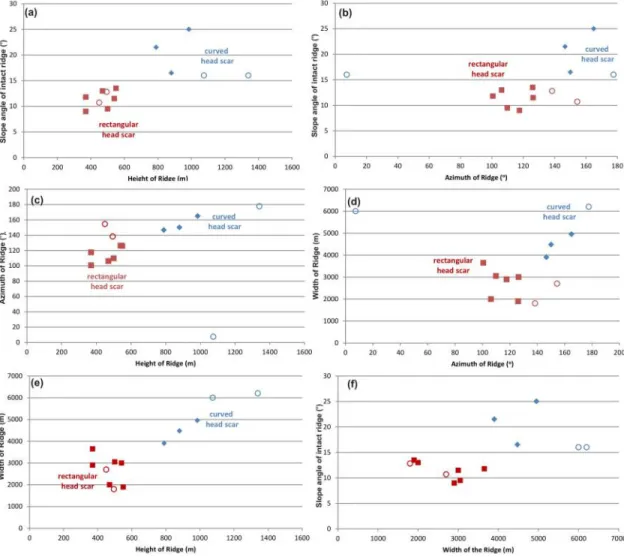
(v) Physiography of ridges
Using the various statistics derived from the bathymetric data (Tables 1 – 3, Figs.
3–5), six cross-plots were generated and summarized in Figure 38. From these distributions, it can be seen that the debris-flow style failures occur on ridges that are more elevated above the abyssal plain and that are steeper than ridges showing blocky failure. Therefore a very simple explanation could be developed to differentiate between the two types of failure systems. Failures initiated at steeper and taller ridges have more potential to generate kinetic forces that can produce the mixing of the sediment down- slope. In contrast, there is less potential kinetic force at ridges with a more gentle slope (less steep and less elevated), resulting in failures with intact sediment blocks. The reasons why the ridges are so different in height and steepness are likely related to the underlying thrust-fault strength and vergence. High elevation may be the result of stronger forces and/or longer time to accumulate uplift. Faster and/or longer times of
68 uplift then could create higher amounts of pore-fluid advection and higher amounts of overpressure. The ridges then have seen failure due to the elevated pore pressure and extensional faults may be created as the sediment pile no longer can withstand the thrust forces and uplift height due to too low internal cohesion.
Figure 38 Cross-plots of physiographic data from the intact ridge systems: (a) slope angle vs. height, (b) slope angle vs. azimuth, (c) azimuth vs. height, (d) width vs.
azimuth, (e) height vs. width, and (f) width vs. slope angle. Failures with rectangular head-scarps are identified by dark-red symbols, while failures with curved head-scars are identified by blue symbols. Open symbols represent failures along the Explorer Plate system of ridges while closed symbols represent failures along the Juan de Fuca.