Modeling the reliability of the Freiburg monosyllabic
speech test in quiet with the Poisson binomial distribution.
Does the Freiburg monosyllabic speech test contain 29 words per list?
Abstract
Every speech test can be modeled as a Bernoulli experiment; this also applies to the Freiburg monosyllabic speech test. The model enables a
Inga Holube
1,2Alexandra Winkler
1,2quantitative calculation of the reliability based on the binomial distribu-
Ralph Nolte-Holube
1tion. Generally, the same probability is assumed for the recognition of each test word. Since the recognition of words within test lists of the
Freiburg monosyllabic speech test differs, modeling with the Poisson 1 Institute of Hearing Technology and Audiology, binomial distribution is reasonable, and results in a narrower confidence
interval than the simple binomial distribution. The variance of the Jade University of Applied Poisson binomial distribution for test lists of the Freiburg monosyllabic Sciences, Oldenburg,
Germany speech test with 20 words can be approximated using the variance of
the simple binomial distribution based on test lists with 29 equally-re-
cognizable words. 2 Cluster of Excellence
“Hearing4All”, Oldenburg, Germany
Keywords:Freiburg monosyllabic test, speech intelligibility, binomial distribution, reliability, confidence
Introduction
The Freiburg monosyllabic speech test (FBE) by Hahlbrock [1] is widely used in speech audiometry and hearing-aid fitting. The result of the speech test (score of correctly repeated words, in %) after performing a test list at a given level by a given person is often regarded as the actual or true value of the person’s speech recognition at this level. However, every speech test is subject to a certain degree of uncertainty, so that the true value (mathematically: the expected value) of a speech-recog- nition score cannot be exactly determined by measuring it once with a test list [2]. Hagerman [3] suggested mod- eling speech tests as Bernoulli processes. In doing so, it is assumed that there is a certain probabilitypjifor each wordifrom the listjthat it will be correctly repeated by the listener. If the same probabilitypj in % can be as- sumed for all words of the test listjat a given level, then the score for speech recognition in percent for this test list (ignoring learning effects and always assuming the same level of attention by the listeners) is subject to the standard deviation:
Equation 1
Winkler and Holube [4] used this standard deviation to estimate the 95% confidence interval for the speech-re-
cognition score of a single test list of the FBE. This is the interval around the true value at which 95% of the measurement results are expected. For the test lists of the FBE with 20 words,n=20. The width of the 95% con- fidence interval can be calculated directly using the bino- mial distribution. Alternatively, and more simply, the nor- mal distribution can be used as an approximation. The width of the 95% confidence interval thus obtained is the standard deviation multiplied by z=1,96. The measure- ment result for a single test list would have to be outside this 95% confidence interval in order to be considered as significantly different.
In the context of an expert interview for the revised ver- sion of the guidelines for assistive devices including hearing aids in Germany, the question was raised as to how many test lists of the FBE are necessary in order to establish a distinguishable hearing ability with a probabil- ity of 95% [5]. One of the interviewed experts commented:
“The approach of a binomial distribution for the Freiburg test is not easy to follow: the probability of correctly recog- nizing a single word depends on the degree of difficulty of each individual word and therefore cannot be set at 0.5. In the Freiburg test, 20 words with different degrees of difficulty are tested in a list.” This statement is based on the everyday experience of working with the FBE, that some words are almost always – and others almost never – understood. Differences in word recognition within the test lists were also described by Hey et al. [6]
for CI patients.
The assumption that all words within a list j have the probabilitypj for correct recognition is thus apparently not true in the FBE. However, the number of correctly re- peated words can be interpreted as a random variable subject to a Poisson binomial distribution. Hagerman [3]
already used the Poisson binomial distribution to account for the variability in word recognition and to estimate its effect on reliability. He was able to show that a test list with 25 words of different recognition has the same reli- ability as a test list with 33 words with equal recognition.
The reason for this effect is that the reliability is worst at a speech-recognition score of 50% and best at 0% and 100%. Hence, the 95% confidence interval is minimal at a speech-recognition score of 0 and 100% and maximal at 50% [4]. Thus if, for example, a word is recognized with a probability of 100%, then it is recognized again and again when it is repeated. However, if the probability is only 50%, then the word is sometimes recognized and sometimes not recognized when it is repeatedly presen- ted. If a test list has a mean speech-recognition score of 50% and all words have the same probability of 50% of being recognized, then the 95% confidence interval for this test list is larger than if some words are well and others are not well recognized. This narrowing of the probability distribution of the number of correctly recog- nized words due to the word recognition variability can also be understood directly as a consequence of Equation 23 in the Appendix (Attachment 1).
In the current analysis, the single word recognition of all 400 words of FBE, which are grouped in 20 test lists, was used in two groups of participants (normal hearing: NH and hearing impaired: HI) to estimate the reliability of the test, taking into account the Poisson binomial distribution.
As a measure of reliability, both the 95% confidence in- terval for the deviation of a measurement from the true value and the 95% confidence interval for the deviation of the true value from a given (measured) value were used.
Methods
Participants
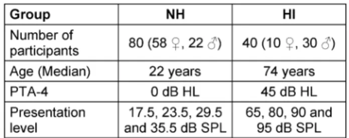
In total, 120 individuals took part in the study. Table 1 gives an overview of the two groups of participants, who were all remunerated for their participation. The pure- tone audiograms according to DIN EN ISO 8253-1 [7]
were measured with an audiometer (Siemens Unity 2) and headphones (Sennheiser HDA 200) in the frequency range from 125 Hz to 8 kHz with all octave and interme- diate (average between octave) frequencies in both ears.
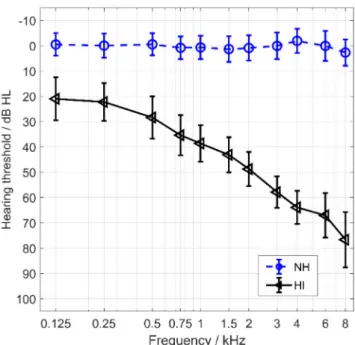
The group NH met the criterion of normal hearing accord- ing to DIN EN ISO 8253-3 [8], i.e. the hearing threshold was at most two frequencies maximally 15 dB HL, and at all other frequencies maximally 10 dB HL. The mean hearing loss (pure tone average, PTA-4) for the frequen- cies 0.5, 1, 2, and 4 kHz is also included as a median for both groups of participants in Table 1. Figure 1 shows
the hearing losses (mean and standard deviation) for both groups. Data from the NH group was already in- cluded in Baljic et al. [9].
Table 1: Overview of groups of participants
Another requirement of DIN EN ISO 8253-3 [8] for the group NH is otological normality. For this purpose, the participants were questioned orally about noise exposure in the 24 hours preceding the test, about taking ototoxic drugs, about hereditary hearing loss, and about their health status. All participants answered these questions with “no” and there were no health restrictions.
The participants of the NH group had had no exposure to the FBE. Since 23 participants of the group HI were fitted with hearing aids, it can be assumed that these participants had performed the FBE several times as part of their hearing-aid fitting process. A training effect can therefore not be excluded for the HI group.
Speech material
The Freiburg monosyllables according to DIN 45621-1 [10] and DIN 45626-1 [11] were presented monaurally via headphones (Sennheiser HAD 200). The ear with the better PTA-4 was used as the measurement ear. For the same PTA-4 for right and left, the measurements were made with the ear typically used for telephoning. The re- cording of 1969 [12] as a digitalization on the Siemens CD (Item No. 7970155 HH 922) was used as speech material. The presentation order of the test words corres- ponded to the word lists specified in DIN 45621-1 [10].
The headphone was calibrated according to DIN EN ISO 60318-1 [13], taking into account the free-field equaliz- ation for the HDA 200 [14] with the calibration signal according toComité Consultatif International Télégraph- ique et Téléphonique (CCITT noise according to ITU-T G.227, [15]). The test words were presented by the Oldenburg Measurement Application (OMA) research version 1.5.5.0 (Hörtech gGmbH). The levels and test lists were randomized.
Word recognition
All participants heard each test list, and thus each word, only once. The test lists were presented at four different levels (see Table 1). Each participant thus listened to five test lists at each level. The assignment of the lists to the levels was different for each participant, so that per level and word, the results of 20 participants of the group NH and 10 participants of the group SH were available. Due
Figure 1: Pure tone thresholds (mean and standard deviation) for both groups of participants NH (blue circles) and HI (black triangles)
to data storage issues, all the test-list results were recor- ded, but the word-specific results were not stored for all measurements. The following data sets were used for the word-specific analysis:
• Group NH:
Test list 9: 77 data sets
•
Test lists 7, 11, 13, 18: 78 data sets
•
All other test lists: 79 data sets
•
• Group HI:
Test lists 3, 9, 13, 15: 39 data sets
•
All other test lists: 40 data sets
•
From the data sets, the word-recognition score in percent was calculated for each word and for each presentation level. Table 2 gives an example for the words “Aas” (car- rion) and “Dorf” (village) of the group HI.
Table 2: Exemplary calculation of word recognition for the words “Aas” and “Dorf”
Results
List-specific word recognition
Figure 2 shows the participant-averaged speech-recogni- tion results for each test list at each level for both groups of participants. The variability of the test lists for the group NH was already reported in detail in [9].
In the current contribution, the differences in word recog- nition within the test lists are of interest. When modeling with the Poisson binomial distribution, every wordiin the test list j is assigned a recognition probabilitypji. Word recognition in percent can be taken as an approximation to the probabilitypji.
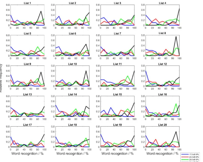
In Figure 3, for each of the 20 test lists for the group NH, the relative frequencies for percent word recognition at the four levels are shown as frequency polygons. For this purpose, the percentage word recognition was divided into classes with a width of 10% each. As a measure of the differences in word recognition, Table 3 shows the root mean square (RMS) of word recognition in percent for each of then=20 test lists at each of the four levels according to:
Equation 2
From Table 3 it can be seen that the percentage of word recognition varied within the test lists to varying degrees.
The largest deviations on average over all four levels were shown in test list 16 with 29 percentage points, the smallest in test lists, 4, 9, 15, and 20 with 20 percentage points. On average across all test lists the RMS value was 23.5 percentage points. For the group HI (not in Table 3), the mean RMS value was 17.4 percentage points (14 percentage points for test lists 14 and 19, and up to 22 percentage points for test list 1). It should be noted, however, that for the group HI the presentation levels were chosen so that the speech recognition, and therefore also the word recognition, was often close to 100% (see Figure 2). In this range, the variance of the measurement results decreases according to Equation 1. Hence, it
Figure 2: The symbols denote speech recognition per list, averaged across the listeners. The dashed lines link speech recognition averaged across all lists at the four presentation levels. Group NH (left) and group HI (right)
Figure 3: Frequency polygons for word recognitionpjifor all listsj (j=1...20) and for all presentation levels for group NH
Table 3: RMS-values of the measured word recognitionpjiin percentages, according to Equation 2; Group NH
cannot be concluded that a hearing impairment leads to a reduction of the variance.
In the Poisson binomial distribution, the expected value of the proportion of correctly recognized words in a test list in percent is given by the mean of the percentage probabilities of the individual words:
Equation 3
The standard deviation in percent of the measurement result for a test listjwith n words of different probability is:
Equation 4
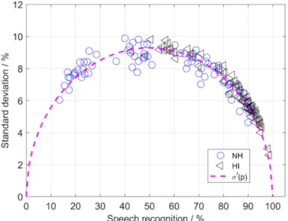
This replaces Equation 1. If the percentage word recogni- tion shown in Figure 3 is used as an approximation for the actually unknown probabilitiespji, then the standard deviationjcan be calculated. The results are plotted for all 20 test lists at all four levels and for both groups of participants in Figure 4, depending on the speech recog- nitionpjof the test lists in %. The observed relative fre- quency (Figure 2) was used for the probabilitypj. It was calculated according to Equation 3 from the average speech recognition of the individual words of test listj.
Approximation with a simple binomial distribution
As in Hagerman [3], the standard deviations jcalculated from the Poisson binomial distribution were approximated by the standard deviation of a simple binomial distribution with a different value n'jinstead of the numbern. This number of wordsn'jis chosen such that a fictitious test list withn'jequally understood words of the probabilitypj has the same standard deviation as the test listj with n=20 words that vary in recognition. This means with Equation 1 and Equation 4:
Equation 5
and therefore Equation 6
This calculation was carried out for each individual test listjwith a distribution in word recognitionpjiand its mean valuepj. Since 20 test lists at four levels were measured for two groups of participants, 160 different values for n'jwere available. These values forn'jwere in the range
Figure 4: Standard deviation calculated using Equation 4 as a function of achieved speech recognitionpjin % for both groups (NH: blue circles, HI: black triangles). The dashed line gives the fitted functionσ'(p) according to Equation 7 obtained from
Equation 1 withn'=29 words (see Equation 9).
of 22–42 with an average of 28 (30 for NH and 27 for HI).
To obtain a common estimate of all conditions, instead of estimating the standard deviation from individual test lists and individual levels, a curve
Equation 7
was fitted to the standard deviationsjplotted in Figure 4.
The value n' is determined by the method of least squares:
Equation 8
The calculation results indΔ/dn'=0 for Equation 9
Here kis the number of test-list measurement results used to calculaten'. If the results of both groups, NH and HI, are included,k=160 (20 test lists at four levels and two groups) and the result is n'=28.7. When fitted for each participant group separately,k=80. For NH alone, n'=29.5 results, and for HI alonen'=27.7. The standard deviation for test lists with 20 words in the FBE can therefore be modeled by the standard deviationσ'of test lists with approximately 29 words having the same word recognition. Using two test lists in the FBE (a total of 40
words) doubles not onlyn, but alson'. The standard devi- ation is inversely proportional to . The relationn'>nis to be expected, because, according to Equation 23 in the Appendix (Attachment 1), the variance of the test-list score becomes smaller due to differences in word-recog- nition probability.
In Equation 7 this is achieved by increasingn'relative to n.
Confidence interval for test-list results
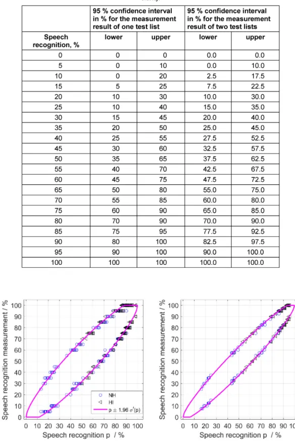
Table 4 gives the bounds of the 95% confidence interval for the result of individual test lists around the true value of speech recognition for n'=29 (one test list with 20 words) andn'=58 (two test lists with, together, 40 words).
The bounds were calculated by multiplyingσ'byz=1.96.
In addition, the 95% confidence interval was determined directly from the Poisson binomial distribution. The distri- bution is explicitly known for each condition (each test listjat all four levels and for both groups of participants), see Equation 20 in the Appendix (Attachment 1). Thus, the confidence interval can be determined symmetrically for each score, starting from the two boundary values (0 words recognized,nwords recognized). Figure 5 shows a good agreement between the two methods. A compar- ison of the bounds in Table 4 with Winkler and Holube [4] shows a shift of the bounds by a maximum of 5 per- centage points when using one test list and by a maximum of 2.5 percentage points when using two test lists. Table 4 shows that for a speech recognition of 50%, doubling the word count from 20 to 40 causes the bounds to shift by 2.5 percentage points each. The 95% con- fidence interval is thus narrowed by 5 percentage points when the number of words is doubled. Thus, for a true speech recognition of 50%, the result of one test list must deviate by at least 20 percentage points to be significantly different, i.e. maximum 30% or at least 70%. In terms of
Table 4: 95% confidence interval for deviations from true values when using one or two test lists. The data was based on the standard deviationσ'(p) according to Equation 7; all values in %; intermediate values for two test lists were omitted for better
clarity.
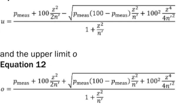
Figure 5: 95% confidence intervals for measured speech recognition with single test lists as a function of the true recognition score. The bounds forp±1.96 · σ'(p) with n'=29 (left) and n'=58 (right) are given as magenta lines. The symbols give the bounds directly obtained from the empirical Poisson binomial distribution for the groups (NH: blue circles, HI: black triangles) when
using one test list (left) and two test lists (right).
statistics, it can then be concluded that the test-list result comes from a different population (with its own true value in speech recognition). Using two test lists, speech-recog- nition scores of 35% or 65%, i.e. a deviation of 15 per- centage points, are significantly different from the as- sumed true value.
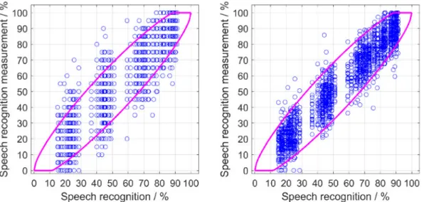
In order to verify the estimate of the 95% confidence in- terval from the binomial distribution, Figure 6 (left) shows the measurement results of group NH for single test lists in addition to the curvesp±1.96·σ'(p)from Figure 5 (left).
The symbols indicate the measurement result for each participant, each test list and each level. These values are given as a function of speech recognition for the test list averaged for all participants at the respective level.
These average values represent an approximation of the true value of speech recognition of the respective test list at the given level. If all participants of the group NH had the same characteristics and abilities, the measure- ment results would be scattered according to the binomial distribution, and 95% of the results would be within the confidence interval (including bounds). However, of the 1,600 test-list results, 261, or 16.31%, are outside the confidence interval. In order to eliminate the variance due to the diversity of the participants, the average over all 20 test lists was used as a simple approach for each participants. The difference between the participant- specific average and the total mean of all measurement result was subtracted from results of the respective par- ticipant. This participant-specific difference is a measure of the characteristics and abilities of each participant relative to the other participants. Corrected measurement results below 0% were limited to 0% and above 100%
were limited to 100% (necessary for a total of 7 measure- ment results). The corrected measurement results are shown in Figure 6 (right). After correction, there are 101 values, i.e. 6.3%, outside the 95% confidence interval.
Confidence interval for the true value
So far, in this contribution, the 95% confidence interval for measured values was calculated around the true value pof a test list using an assumed probability distribution.
However, this true value is unknown. Another question is, in which range would this true valueplie with a prob- ability of 95%, if only the measurement resultpmeasfor a single test list were available. Frequently, Equation 1 is also used to calculate this 95% confidence interval.
Wilson [16] used the following approach for the limits of the 95% confidence interval for the true value with z=1.96:
Equation 10
Instead ofn, the valuen'was used in the present investi- gation (n'=29 forn=20,n'=58 forn=40). This takes into account the smaller width of the Poisson binomial distri-
bution compared to the simple binomial distribution.
Solving forpyields the lower limitu Equation 11
and the upper limito Equation 12
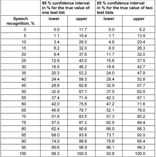
The method for calculating the 95% confidence intervals for the true value around the measurements according to Equation 11 and Equation 12 was recommended by Altman et al. [17] and Brown et al. [18]. The results are shown in Figure 7 forn'=29 andn'=58.
Table 5 indicates the bounds thus obtained as numerical values. Since the true value in speech recognition is not limited by any measurement resolution, i.e. 5% steps when using 20 words and 2.5% steps when using 40 words, a corresponding rounding was omitted here. The largest differences compared to Table 4 are found at speech-recognition scores of 0% and 100%. The width of the confidence interval for the true value is larger than zero at these positions. For a test-list score of 80% using a 20-word test list, the true value of speech recognition lies in the range from 62.4% to 90.6% is with a probability of 95%. In addition, with a test list score of 90%, the true speech-recognition value can also be less than 80% with considerable probability. Even with the use of two test lists, the lower 95% confidence limit for the true value is still just under 80% for a measured speech recognition of 90%.
Discussion
In the current contribution, the FBE was modeled with a Poisson binomial distribution to account for the varying word recognition within the test lists. The modeling al- lowed the Poisson binomial distribution of the 20-word FBE test lists to be approximated by a simple 29-word binomial distribution. Thus, the results of Hagerman [3]
were qualitatively confirmed. He derived a similar increase in the number of test items fromn=25 ton‘=33. When applied to the underlying measurement data, after elim- ination of participant’s variability by a global, participant- specific correction value, 6.3% of the measurement res- ults were outside the 95% confidence interval. This pro- portion is surprisingly close to the 5% expected theoretically to be outside the confidence interval. In do- ing so, other sources of variance, such as the fluctuating attention of the participants and of the examiner from test list to test list were not considered.
Equation 23 (see Attachment 1), which describes the re- lationship between the variances of a simple and a Pois-
Figure 6: The circle symbols show the speech-recognition score for single test lists versus the average of the test list for all participants of group NH at a given level. The variance due to the differences between the participants was eliminated in the
right side of the figure. As a comparison, the magenta lines give the 95%-confidence interval according to Figure 5(left).
Figure 7: 95% confidence intervals for the true score as a function of a measured score, based on Wilson [16], Equation 11 and Equation 12 in comparison to the 95% confidence interval for measured scores relative to the true speech recognition
according top±1.96 · σ'(p), as shown in Figure 5.
son binomial distribution with the same expectation value, leads to the conclusion that the reliability of a speech test improves with increasing inequality of test items in speech recognition. In an extreme case, a test list could consist only of words that are understood either always (i.e. with a probability of 100%) or never (i.e. with a probability of 0%). This measurement result could be re- produced with certainty. Here it becomes clear that nar- row confidence intervals or a high reliability alone are not sufficient for evaluating a speech test. The aim of a speech test is to establish speech recognition as a func- tion of the presentation level, to determine the success of a rehabilitation approach, or to compare different provisions with technical hearing devices. This requires the measurement of the course of the discrimination function, or specific points on the discrimination function, as accurately as possible. These goals cannot be achieved with test items that are either not recognized at all or are always recognized. A good speech test is not only charac- terized by high reliability or narrow 95% confidence inter-
vals. It should also have a high sensitivity to level changes, for disability due to hearing loss, and for the effects of rehabilitation or care. These criteria were not quantitatively investigated in the present study. It should be noted, however, that a higher variation in word recog- nition within a test list leads to a flatter slope of the dis- crimination function for this list [19]. In [9] the test list- specific discrimination functions for the data of the NH group were given. The slope was only 4.5 percentage points per dB. In this sense, the variability of word recog- nition within a test list makes it possible to increase reli- ability and to decrease sensitivity. In order to increase the measurement accuracy of the FBE, the modified guidelines for assistive devices describe the use of two test lists. Doubling the number of words reduces the 95%
confidence intervals. However, even with the Poisson bi- nomial distribution, the reduction is not linear with the number of wordsn, but linear with and thus does not change as much as would be desirable for a doubling of the measurement effort.
Table 5: 95% confidence interval for deviations of the true value from the measurement result when using one or two test lists.
Given are confidence intervals based on Wilson [16]; Equation 11 and Equation 12. All values in %. Intermediate values for two test lists were omitted for better clarity.
Regarding the application of the analysis with regard to the guidelines for assistive devices, it has to be taken into account that the 95% confidence intervals calculated with the Poisson binomial distribution apply only to the FBE in quiet. The distribution of word recognition within the test lists for the FBE in noise is not yet known and may lead to a different reliability. If the distribution is wider, it will result in a reduction of the 95% confidence interval; if narrower, the 95% confidence interval will be increased. Furthermore, it should be noted that the ana- lyses only show the 95% confidence intervals for the de- viations of measured values from the true value, and for the deviations of the true value from a measured value.
However, 95% confidence intervals of the difference of two measured scores are different variables that are needed to obtain the test-retest reliability. Here, the variances of the two individual measurements add up [20]. The test-retest reliability is relevant for the assess- ment of the comparison of the conditions with and without hearing aids, or of two hearing aids, or their settings.
Therefore, the confidence intervals reported in this article cannot be used to compare with the requirements in the guideline (improvement by 20% in quiet and 10% in noise). This will be covered in a future contribution.
Notes
Publication note
This contribution was previously published in German as:
Holube I, Winkler A, Nolte-Holube R. Modellierung der Reliabilität des Freiburger Einsilbertests in Ruhe mit der verallgemeinerten Binomialverteilung. Z Audiol.
2018;57(1):6-17.
Acknowledgement
This study was funded by the Ph.D. program Jade2Pro of Jade University of Applied Sciences. The authors thank Daniel Berg (HörTech gGmbH) for technical support as well as Sascha Bilert, Lena Haverkamp, Miriam Kropp, and Florian Wiese for their support in data acquisition.
English language services were provided by stels-ol.de.
Competing interests
The authors declare that they have no competing in- terests.
Attachments
Available from
https://www.egms.de/en/journals/zaud/2020-2/zaud000005.shtml 1. Attachment1_zaud000005.pdf (169 KB)
Attachment1: Poisson binomial distribution
References
1. Hahlbrock K. Über Sprachaudiometrie und neue Wörterteste.
Archiv f. Ohren-, Nasen- u. Kehlkopfheilkunde.
1953;162:394–431. DOI: 10.1007/BF02105664 2. Egan JP. Articulation testing methods. Laryngoscope. 1948
Sep;58(9):955-91. DOI: 10.1288/00005537-194809000-00002 3. Hagerman B. Reliability in the determination of speech
discrimination. Scand Audiol. 1976;5:219-28. DOI:
10.3109/01050397609044991
4. Winkler A, Holube I. Test-Retest-Reliabilität des Freiburger Einsilbertests [Test-retest reliability of the Freiburg monosyllabic speech test]. HNO. 2016 Aug;64(8):564-71. DOI:
10.1007/s00106-016-0166-2
5. Gemeinsamer Bundesausschuss. Tragende Gründe zum Beschluss des Gemeinsamen Bundesausschusses über eine Änderung der Hilfsmittel-Richtlinie: Freiburger Einsilbertest im Störschall. 24. November 2016. [accessed 05.06.2017].
Verfügbar unter: https://www.g-ba.de/informationen/
beschluesse/2758/
6. Hey M, Brademann G, Ambrosch P. Der Freiburger Einsilbertest in der postoperativen CI-Diagnostik [The Freiburg monosyllable word test in postoperative cochlear implant diagnostics]. HNO.
2016 Aug;64(8):601-7. DOI: 10.1007/s00106-016-0194-y 7. DIN EN ISO 8253-1. Akustik – Audiometrische Prüfverfahren –
Teil 1: Grundlegende Verfahren der Luft- und Knochenleitungs- Schwellenaudiometrie mit reinen Tönen. Berlin: Beuth Verlag;
2011.
8. DIN EN ISO 8253-3. Akustik – Audiometrische Prüfverfahren – Teil 3: Sprachaudiometrie. Berlin: Beuth Verlag; 2012.
9. Baljić I, Winkler A, Schmidt T, Holube I. Untersuchungen zur perzeptiven Äquivalenz der Testlisten im Freiburger Einsilbertest [Evaluation of the perceptual equivalence of test lists in the Freiburg monosyllabic speech test]. HNO. 2016 Aug;64(8):572- 83. DOI: 10.1007/s00106-016-0192-0
10. DIN 45621-1. Sprache für Gehörprüfung. Teil 1: Ein- und mehrsilbige Wörter. Berlin: Beuth Verlag; 1995.
11. DIN 45626-1. Tonträger mit Sprache für Gehörprüfung, Teil 1:
Tonträger mit Wörtern nach DIN 45621-1. Berlin: Beuth Verlag;
1995.
12. Brinkmann K. Die Neuaufnahme der „Wörter für Gehörprüfung mit Sprache“. Z Hörgeräteakustik. 1974;13:12-40.
13. DIN EN 60318-1. Akustik – Simulatoren des menschlichen Kopfes und Ohres – Teil 1: Ohrsimulator zur Kalibrierung von supra-auralen und circumauralen Kopfhörern. Berlin: Beuth Verlag; 1999.
14. DIN EN ISO 389-8. Akustik – Standard-Bezugsschwellenpegel für die Kalibrierung audiometrischer Geräte – Teil 8: Äquivalente BezugsSchwellenschalldruckpegel für reine Töne und circumaurale Kopfhörer. Berlin: Beuth Verlag; 2004.
15. ITU. ITU-T Recommendation G.227. Conventional telephone signal. Genf: ITU; 1993.
16. Wilson EB. Probable inference, the law of succession, and statistical interference. Journal of the American Statistical Association. 1927;22(158):209-212. DOI:
10.1080/01621459.1927.10502953
17. Altman DG, Machin D, Bryant TN, Gardner MJ. Statistics with confidence. BMJ Books. 2nd ed. 2000.
18. Brown LD, Cai TT, DasGupta A. Interval estimation for a binomial proportion. Statistical Science. 2001;16(2):101-117. DOI:
10.1214/ss/1009213286
19. Kollmeier B, Warzybok A, Hochmuth S, Zokoll MA, Uslar V, Brand T, Wagener KC. The multilingual matrix test: Principles, applications, and comparison across languages: A review. Int J Audiol. 2015;54 Suppl 2:3-16. DOI:
10.3109/14992027.2015.1020971
20. Thornton AR, Raffin MJ. Speech-discrimination scores modeled as a binomial variable. J Speech Hear Res. 1978 Sep;21(3):507- 18. DOI: 10.1044/jshr.2103.507
21. Wang YH. On the number of successes in independent trials.
Statistica Sinica. 1993;3:295-312.
22. Hong Y. On computing the distribution function for the Poisson binomial distribution. Computational Statistics & Data Analysis.
2013;59:41-51. DOI: 10.1016/j.csda.2012.10.006
Corresponding author:
Prof. Dr. Inga Holube
Jade Hochschule, Institut für Hörtechnik und Audiologie, Ofener Str. 16/19, D-26121 Oldenburg
Inga.Holube@jade-hs.de
Please cite as
Holube I, Winkler A, Nolte-Holube R. Modeling the reliability of the Freiburg monosyllabic speech test in quiet with the Poisson binomial distribution. Does the Freiburg monosyllabic speech test contain 29 words per list? GMS Z Audiol (Audiol Acoust). 2020;2:Doc01.
DOI: 10.3205/zaud000005, URN: urn:nbn:de:0183-zaud0000059
This article is freely available from
https://www.egms.de/en/journals/zaud/2020-2/zaud000005.shtml Published:2020-03-23
Copyright
©2020 Holube et al. This is an Open Access article distributed under the terms of the Creative Commons Attribution 4.0 License. See license information at http://creativecommons.org/licenses/by/4.0/.