Algorithmic Model Theory SS 2010

(1)

Algorithmic Model Theory SS 2010

Prof. Dr. Erich Grädel

(2)

cbnd

This work is licensed under:

http://creativecommons.org/licenses/by-nc-nd/3.0/de/

Dieses Werk ist lizenziert unter:

http://creativecommons.org/licenses/by-nc-nd/3.0/de/

http://www.logic.rwth-aachen.de

(3)

1 The classical decision problem for FO

The classical decision problem for first-order logic was considered the main problem of mathematical logic by Hilbert and Ackermann and its undecidability was shown by Church and Turing.

The Entscheidungsproblem is solved when we know a procedure that allows for any given logical expression to decide by finitely many operations its validity or satisfiability. [. . . ] The Entscheidungsproblem must be considered the main problem of mathematical logic.

(D. Hilbert and W. Ackermann, 1928) We introduce the classical decision problem for first-order logic, for which we present three equivalent formulations. The importance of the decision problem for first-order logic results from the fact that first-order logic provides a framework to express almost all aspects of mathematics.

Satisfiability: Construct an algorithm that decides for any given formula of FO whether it has a model.

Validity: Construct an algorithm that decides for any given formula of FO whether it is valid, i.e. whether it holds in all models where it is defined.

Provability: Construct an algorithm that decides for any given formula ψof FO whether ⊢ψ, meaningψis provable from the empty set of axioms in some formal system, e.g. sequential calculus.

Sinceψis satisfiable if and only if¬ψis not valid, satisfiability and validity are equivalent problems with respect to computability. The equivalence with provability is a much more intricate result and in fact a consequence of the following

(6)

1 The classical decision problem forFO

Theorem 1.1(Completeness Theorem (Gödel)). For any given set of sentencesΦ⊆FO(τ)and any sentenceψ∈FO(τ)it holds that

Φ|=ψ ⇐⇒ _Φ⊢ψ; in particular∅|=ψ⇔_∅⊢ψ.

As a direct consequence we get the following

Theorem 1.2. The set of valid first-order formulae is recursively enumerable.

1.1 Basic notions on decidability

In our formulation of the decision problem it was not precisely specified what an algorithm is. It was not until the 1930s that Church and Kleene , Gödel and Turing provided a precise definition of an abstract algorithm.

Their approaches are today known to be equivalent. We introduce the concept of a Turing machine.

Definition 1.3. ATuring machine(TM)Mis a 6-tuple M= (Q,Σ,Γ,q₀,F,δ), where

• Qdenotes a finite set of states,

• Σ,Γdenote finite alphabets, whereΣis the working alphabet with a special blank symbol∈_Σ,

• Γ⊆Σ\ {}is the input alphabet,

• q₀∈Qdenotes the initial state,

• F⊆Qis the set of final states and

• δ:(Q\F)×Σ→Q×Σ× {−1, 0, 1}is the transition function.

Aconfigurationis an elementC= (q,p,w=w₀w₁. . .w_k)∈Q×_N×_Σ^∗. The transition function δinduces a partial function on the set of all configurations

C7→Next(C),

where for δ(q,wp) = (q^′,a,m), the successor configuration of C is defined as Next(C) = (q^′,p+m,w₀. . .wp−1aw_p+1· · ·w_k). Acom- putation of the TM M on an input word x ∈ Γ^∗ is a configuration

2

(7)

sequence C₀,C₁, . . .

whereC₀ =C₀(x)_:= (q₀, 0,x)is the input configuration andC_i+1 = Next(C_i)for alli.

M haltsonxif the computation ofMonxis finite, i.e. ends in a final configurationC_f = (q,p,w)withq∈F.

The language accepted byMis L(M):={x∈_Γ^∗:Mhalts onx}.

Mcomputes a partial function f_M:Γ^∗ →Σ^∗with domainL(M) such that f_M(x) =yif and only if the computation ofMonxends in (q,p,y)for someq∈F,y∈_Σ^∗andp∈_N.

Definition 1.4. ATuring acceptor is a Turing machine M with F = F⁺∪·F⁻whereM accepts xif the computation ofMonxends in a state inF⁺. M rejects xif the computation ofMonxends in a state inF⁻. Definition 1.5.

• L⊆_Γ^∗ isrecursively enumerable (r.e.) if there exists a TMMwith L(M) =L.

• L⊆_Γ^∗isco-recursively enumerable (co-r.e.)ifL:=_Γ^∗\Lis r.e..

• A (partial) function f :Γ^∗→Σ^∗is(Turing) computableif there is a TMMwith f_M= f.

• L⊆_Γ^∗isdecidableif there is a Turing acceptorMsuch that for all x∈Γ^∗

x∈L⇒Macceptsx x∈/L⇒Mrejectsx

or, equivalently,Lis decidable if its characteristic function χL:Γ^∗→ {0, 1}is Turing computable.

Theorem 1.6. A language L ⊆ Γ^∗ is decidable if and only ifL is r.e.

and co-r.e.

(8)

Definition 1.7. Let A ⊆ Γ^∗,B ⊆ Σ^∗. We say that Ais(many-to-one) reducibletoB,A≤B, if there is a total computable functionf :Γ^∗→_Σ^∗ such that for allx∈_Γ^∗ we havex∈A⇔ f(x)∈B.

Lemma 1.8.

• A≤B,Bdecidable⇒Adecidable

• A≤B,Br.e. ⇒Ar.e.

• A≤B, Aundecidable⇒Bundecidable.

There surely are undecidable languages since there are only count- ably many Turing machines but uncountably many languages. Un- fortunately, among these languages there are quite relevant classes of languages. For example we cannot even decide whether a TM halts on a given input.

Definition 1.9(Halting Problems). Thegeneral halting problemis defined as

H:={ρ(M)#ρ(x):MTuring machine,x∈L(M)}

whereρ(_M)_and_ρ(_x)are encodings of the TMMand the inputxover a fixed alphabet{0, 1}such that the computation of Mon xcan be reconstructed from the encodingsρ(M)andρ(x)in an effective way.

There is a universal TMUwhich, givenρ(M)andρ(x), simulates the computation ofMonxand halts if and only ifMhalts onx. Thus, L(U) =Hfrom which we conclude thatHis r.e..

We introduce two special variants of the halting problem

• Self-application problem

H₀:={ρ(M):ρ(M)∈L(M)}

• Halting on the empty word H_ε:={ρ(M):ε∈L(M)}

Theorem 1.10. H,H₀,Hεare undecidable.

4

(9)

Proof.

• H₀is not co-r.e. and thus undecidable. OtherwiseH₀=L(M₀)for some TMM₀. Then

ρ(M₀)∈H₀⇔M₀halts onρ(M₀)⇔ρ(M₀)∈H₀.

• H₀is a special case ofH,H₀≤H, and thusHis undecidable.

• We can reduceHtoH_ε, thusH_εis undecidable. q.e.d. As a consequence of the next theorem we cannot algorithmically prove whether a program computes a given function, i.e. we cannot algorithmically prove the correctness of a program. Note that this does not mean that we cannot prove the correctness of a single given program. Instead the statement is that we cannot do so algorithmically for all programs.

Theorem 1.11(Rice). LetRbe the set of all computable functions and letS⊆ Rbe a set of computable functions such thatS̸=_∅andS̸=R. Then code(S):={ρ(M): fM∈S}is undecidable.

Proof. Let⇑be the everywhere undefined function, i.e. Def(⇑) =_∅.

Obviously,⇑is computable. Assume that⇑̸∈S (otherwise consider R \S instead of S. Clearly if code(R \S) is undecidable then so is code(S).)

As S ̸=∅, there exists a function f ∈ S . LetM_f be a TM that computes f, i.e. f_M_f = f. We define a reduction H_ε ≤ code(S)by describing a total computable functionρ(M)7→ρ(M^′)such that

Mhalts onε⇔ fM^′ ∈S.

Specifically, givenρ(M), we construct the encoding of a TMM^′which, given an inputx, proceeds as follows:

• first simulateMonε(i.e. apply the universal TMUtoρ(M)#ε);

• then simulate M_f on x (i.e. apply the universal TM U to ρ(M_f)_#ρ(x)_).

(10)

It is clear that the reduction function is computable. Furthermore, ifMhalts onεthen f_M^′(x) = f(x) for all inputsx, i.e. f_M^′ = f, so f_M^′ ∈S. IfMdoes not halt onεthenM^′does not halt onxfor anyx,

i.e. f_M^′ =⇑, so f_M^′ ̸∈S. q.e.d.

Definition 1.12(Recursive inseparability). LetA,B⊆Γ^∗be two disjoint sets. We say thatAandBarerecursively inseparableif there exists no recursive setC⊆_Γ^∗such thatA⊆CandB∩C=_∅.

Example. (_A,_A)are recursively inseparable if and only ifAis undecidable.

Lemma 1.13. LetA,B⊆_Γ^∗,A∩B=_∅be recursively inseparable. Let X,Y⊆Σ^∗,X∩Y =_{∅, and let} f be a total computable function such thatf(A)⊆Xand f(B)⊆Y. ThenXandYare recursively inseparable.

Proof. Assume there exists a decidable setZ ⊆_Σ^∗ such thatX ⊆ Z andY∩Z=∅. ConsiderC={x∈ _Γ^∗ : f(x) ∈ Z}. Cis decidable, A⊆C,B∩C=_{∅, thus}CseparatesA,B. q.e.d. Notation:We write(A,B)≤(X,Y)if such a function f exists.

Example. (A,A)≤(B,B)⇔A≤B.

As a preparation to prove Trakhtenbrot’s theorem, we consider a refinement ofH_ε

H⁺_ε :={ρ(M):Macceptsε} H⁻_ε :={ρ(M):Mrejectsε}

H_ε^∞:={ρ(M): the computation ofMonεis infinite and does not cycle.}

H₀⁺, H₀⁻, H₀^∞ are defined analogously, with respect to self- application.

Theorem 1.14. H⁺_ε ,H⁻_ε andH_ε^∞are pairwise recursively inseparable.

Proof.

6

(11)

• (H_ε⁺,H^∞_ε ): We show that every setCwithH_ε⁺⊆Cand H_ε^∞∩C=

∅is undecidable by reducing the halting problemH_εtoC. Define the functionρ(M)7→ρ(M^′)as follows. From a given codeρ(M) construct the code of a TMM^′that simulatesMand simultaneously counts the number of computation steps since the start. IfMhalts (accepting or rejecting),M^′accepts.

It is clear that the reduction function is computable. IfMhalts onε thenM^′halts onεas well and accepts, soρ(M^′)∈H⁺_ε ⊆C. IfM does not halt onεthenM^′does not halt either, soρ(M^′) ∈ H_ε^∞ and asH_ε^∞∩C=_{∅, we have}ρ(M^′)̸∈C.

• The statement forH⁻_ε andH_ε^∞is proven analogously.

• (H_ε⁻,H⁺_ε ): Show that(H₀⁻,H₀⁺) ≤(H_ε⁻,H_ε⁺)and that (H₀⁻,H₀⁺) are recursively inseparable.

– (H₀⁻,H₀⁺)≤(H⁻_ε ,H_ε⁺):

For a given input TMMconstruct a TMM^′that ignores its own input and simulatesMonρ(M). Obviously,M^′ can be constructed effectively, say by a computable functionh. Now h(M) acceptsεiff Macceptsρ(M)andh(M)rejectsεiffM rejectsρ(M)_.

– (H₀⁻,H₀⁺)recursively inseparable:

Assume there exists a decidableCwithH₀⁻⊆CandH⁺₀ ⊆C.

Consider a machineM₀that decidesC. There are two cases:

(1) M0acceptsρ(M0). Thenρ(M0)∈Cby definition ofM0. Thenρ(M₀)̸∈H₀⁺by definition ofC. On the other hand, ifM₀ acceptsρ(M₀)thenρ(M₀)∈H₀⁺ (by definition of H₀⁺), a contradiction.

(2) M₀rejectsρ(M₀). Thenρ(M₀) ̸∈Cby definition ofM₀. Thenρ(M₀)̸∈H₀⁻by definition ofC. On the other hand, ifM0 rejectsρ(M0)thenρ(M0) ∈ H₀⁻ (by definition of H₀⁻), a contradiction.

q.e.d.

(12)

1.2 Trakhtenbrot’s Theorem

In the following, we consider FO, more precisely first-order logic with equality. We restrict ourselves to a countable signature

τ_∞:={Rⁱ_j:i,j∈_N} ∪ {f_jⁱ:i,j∈_N}

whereRⁱ_j stands for a relation symbol of arity iand f_jⁱ stands for a function symbol of arityi.

We encode formulae over a fixed alphabet Γ:={R,f,x, 0, 1,[_,]} ∪ {=,¬,∧,∨,→,↔,∃,∀.(_,)}, and uniquely encode the relational and functional symbols

relation symbols: Rⁱ_j 7−→ R[_bini][_binj] functional symbols: f_jⁱ 7−→ f[bini][binj]

variables: x_j 7−→ x[binj].

Thus, every formulaϕ∈FO is a word inΓ^∗.

Let X ⊆ FO be a class of formulae. We analyse the following decision problems:

Sat(X):={ψ∈X:ψhas a model} Fin-sat(X):={ψ∈X:ψhas a finite model}

Val(X):={ψ∈X:ψis valid} Non-sat(X):=X\Sat(X)

Inf-axioms(X):=Sat(X)\Fin-sat(X)

={ψ∈X: ψis an infinity axiom, i.e.ψhas a model but no finite model}. Theorem 1.15. LetX⊆FO be decidable. Then

(1)Val(X)is r.e.

(2)Non-sat(X)is r.e.

(3)Sat(X)_{is co-r.e.}

8

(13)

(4) Fin-sat(X)_{is r.e.}

(5) Inf-axioms(X)is co-r.e.

Proof. (1) ϕis valid⇔ ⊢ ϕ(Completeness Theorem). Thus we can systematically enumerate all proofs and halt if a proof for ϕis listed.

(2) ϕvalid⇔ ¬ϕis not satisfiable.

(3) Follows from Item (2).

(4) Systematically generate all finite models and halt if a model ofϕis found.

(5) FO\Inf-axioms(X) =Non-sat(X)∪Fin-sat(X)is r.e. q.e.d. Definition 1.16. A classX⊆FO has thefinite model property(FMP) if every satisfiableϕ∈Xhas a finite model, i.e. ifSat(X) =Fin-sat(X)_. Theorem 1.17. Suppose thatX⊆FO is decidable and thatXhas the FMP. ThenSat(X)is decidable.

Proof. Sat(X)is co-r.e. and sinceSat(X) =Fin-sat(X)andFin-sat(X)is r.e. alsoSat(X)is r.e. ThusSat(X)is decidable. q.e.d. In this case alsoFin-sat(X),Non-sat(X),Val(X)are decidable and of courseInf-axioms(X) =_∅is decidable.

Theorem 1.18 (Trakhtenbrot). There is a finite vocabulary τ ⊆ τ_∞ such that Fin-sat(FO(τ)),Non-sat(FO(τ)) and Inf-axioms(FO(τ)) are pairwise recursively inseparable and therefore undecidable.

The proof of Trakhtenbrot’s theorem introduces a proof strategy that can be applied in many other undecidability proofs. (Do not focus on the technicalities but on the general idea to construct the reduction formulae.)

Proof. LetMbe a deterministic Turing acceptor. We show that there is an effective reductionρ(M)7→ψ_Msuch that

(1) Macceptsε =⇒ ψ_Mhas a finite model.

(2) Mrejectsε =⇒ ψMis unsatisfiable.

(14)

(3) The computation ofMonεis infinite and non-periodic =⇒ ψM

is an infinity axiom.

Then the theorem follows by Lemma 1.13.

LetMbe a Turing acceptor with statesQ={q₀, . . . ,qr}, initial state q0, alphabetΣ={a0, . . . ,as}(wherea0=), final statesF=F⁺∪F⁻ and transition functionδ.

ψMis defined over the vocabularyτ={0,f,q,p,w}where 0 is a constant,f,q,pare unary functions andwis a binary function. Define the termkas f^k0.

By constructing a formula we intend to have a model A_M = (A, 0,f,q,p,w)describing a run ofMon the inputεwhere

• universeA={0, 1, 2, . . . ,n}orA=_N;

• f(t) =t+1 ift+1∈Aandf(t) =t, iftis the last element ofA;

• q(t) =iiffMis at timetin stateq_i;

• p(t)is the head position ofMat timet;

• w(s,t) =iiff symbola_iis at timeton tape-cells.

Note that we cannot enforce this model, but ifψ_Mis satisfiable this one will be among its models.

ψM:= _START ∧ COMPUTE ∧ END START := (q0=0∧p0=0∧ ∀x w(x, 0) =0).

[Enforces input configuration onεat time 0]

COMPUTE :=NOCHANGE∧ CHANGE

NOCHANGE :=∀x∀y(py̸=x→w(x,f y) =w(x,y))

[content of currently not visited tape cells does not change]

CHANGE := ^{^}

δ:(qi,aj)7→(q_k,aℓ,m)

∀y(α_i,j→β_k,ℓ,m) where

αij:= (qy=i∧w(py,y) =j)

[Mis at timeyin stateqiand reads the symbolaj] β_k,ℓ,m:= (q f y=k∧w(py,f y) =ℓ∧MOVEm)

10

(15)

and

MOVEm:=











p f y=py ifm=0 p f y=f py ifm=1

∃z(f z=py∧p f y=z) ifm=−1.

END := ^{^}

δ(qi,aj)undef.

qi̸∈F⁺

∀y¬α_ij

[The only way the computation ends is in an accepting state]

Remark1.19.

• ρ(M)7→ψMis an effective construction.

• IfMacceptsε, the intended model is finite and is indeed a model A_M|=ψ_M, thusψ_M∈Fin-sat(FO(τ)).

• If the computation ofM on εis infinite, the intended model is infinite andA_M|=ψM.

It remains to show that ifMrejectsε, thenψMis unsatisfiable, and if the computation of Monεis infinite and aperiodic, thenψ_Mis an infinity axiom.

SupposeB= (B, 0,f,q,p,w)|=ψ_M.

Definition 1.20. Benforces at timet the configuration (q_i,j,w) with w=a_i₀. . .a_i_m∈_Σ^∗if

(1) B|=qt=i, (2) B|=pt=j,

(3) for allk≤m,B|=w(k,t) =i_kand for allk>m,B|=w(k,t) =0.

SinceB|=ψ_M, the following holds:

• BenforcesC₀= (q₀, 0,ε)at time 0 (sinceB|= START.)

• IfBenforces at timeta non-final configurationCt, thenBenforces the configurationC_t+1=Next(Ct)at timet+1.

• Especially, the computation ofMcannot reach a rejecting configuration. It follows that ifMrejectsε, thenψMis unsatisfiable.

(16)

Consider an infinite and aperiodic computation ofM, and assume B|=ψ_Mis finite. SinceBis finite, it enforces a periodic computation in contradiction to the assumption that the computation ofM is aperiodic.

C₀⊢. . .⊢ Cr ⊢. . .⊢ Ct−1

We have shown:

• IfMacceptsε, thenψMhas a finite model.

• IfMrejectsε, thenψMis unsatisfiable.

• If the computation of Mis infinite and aperiodic, thenψ_Mis an

infinity axiom. q.e.d.

We now know that the sets of all finitely satisfiable, all unsatisfiable and all only infinitely satisfiable formulae are undecidable for FO(_τ) whereτconsists of only three unary functions and one binary function.

This raises a number of questions.

(1) For which other vocabulariesσdo we have similar undecidability results for FO(σ)?

(2) For whichσis satisfiability of FO(σ)decidable?

(3) Is there a complete classification? In this case, we want to find min- imal vocabulariesσsuch that the above problems are undecidable, i.e. vocabularies such that any further restriction yields a class of formulae for which satisfiability is decidable.

We first define what it means that a fragment of FO is as hard for satisfiability as the whole FO.

Definition 1.21. X⊆FO is areduction classif there exists a computable functionf : FO→Xsuch thatψ∈Sat(_FO)⇔ f(_ψ)∈Sat(X)_.

LetX,Y⊆FO. Aconservative reduction of X to Yis a computable functionf :X→Ywith

• ψ∈Sat(X)⇔ f(ψ)∈Sat(Y), and

• ψ∈Fin-sat(X)⇔ f(_ψ)∈Fin-sat(Y)_.

12

(17)

Xis aconservative reduction classif there exists a conservative reduction of FO toX.

Corollary 1.22. Let X be a conservative reduction class. Then Fin-sat(X),Inf-axioms(X)andNon-sat(X)are pairwise recursively inseparable, and thus Fin-sat(X), Sat(X),Val(X),Non-sat(X),Inf-axioms(X) are undecidable.

Proof. A conservative reduction from FO toXyields a uniform reduction fromFin-sat(FO), Inf-axioms(FO) andNon-sat(FO) toFin-sat(X), Inf-axioms(X)andNon-sat(X), respectively. q.e.d. We now observe that we can indeed give a complete classification of signaturesσsuch that FO(_σ)is decidable.

Theorem 1.23. If σ ⊆ {P₀,P₁, . . .} ∪ {f} consists of at most one unary function f and an arbitrary number of monadic relations P₀,P₁, . . ., thenSat(_FO(_σ))is decidable. In all other cases,Sat(_FO(_σ))_, Inf-axioms(FO(σ))andNon-sat(FO(σ))are pairwise recursively inseparable, and FO(σ)is a conservative reduction class.

A full proof of this classification theorem is rather difficult. In particular, the decidability of the monadic theory of one unary function, which implies the decidability part, is a difficult theorem due to Rabin.

On the other side, one has to show that Trakhtenbrot’s theorem applies to the vocabularies

τ1={E}whereEis a binary relation, τ₂={f,g}where f,gare unary functions, τ3={F}whereFis a binary function, and hence to all extensions ofτ₁,τ₂,τ₃.

Of course, we may also look at other syntactic restrictions besides restricting the vocabulary. One possibility is to restrict the number of variables. This is only interesting for relational formulae. If we have functions, satisfiability is undecidable even for formulae with only one variable as we shall see.

Define FO^kas first-order logic with relational symbols only and a fixed amount ofkvariables, sayx₁, . . . ,x_k.

(18)

Theorem 1.24.

• FO²has the finite model property and is decidable (see Chapter 2).

• FO³is a conservative reduction class.

Another possibility is to restrict the structure of quantifier prefixes.

Definition 1.25(Prefix-Vocabulary Classes). A string in{∀,∃}^∗is called prefix, and anarity sequenceis a sequence assigning all positive integers values inN∪ {ω}.

For any set of prefixesΠand any arity sequencespand f,[_Π,p,f] and[_Π,p,f]₌denote the collection of all formulae ϕ∈FO in prenex normal form without equality and with equality, respectively, such that

• the prefix ofϕbelongs toΠ,

• the number ofn-ary predicate symbols inϕis at mostp(n)_and

• the number ofn-ary function symbols inϕis at most f(n).

• Except for the logical constants trueand false, ϕ has no nullary predicate symbols, no nullary function symbols and no free variables.

The prefix set containing all prefixes and the arity sequence that assigns ωto eachnwill be denotedall.

We write arity sequences as tuples, e.g.,(2, 1,ω),(0)to express that two predicate symbols of arity 1, one of arity 2, unboundedly many of arity 3 and no other predicate or function symbols are allowed.

Theorem 1.26 (Gurevich). Let Xbe a prefix class, p,q two arity sequences andX= [_Π,p,q]₌.

• Xis a conservative reduction class if it contains any of (1) [∀,(0),(2)]₌

(2) [∀,(0),(0, 1)]₌ (3) [∀²∃,(ω, 1),(0)]₌ (4) [∃^∗∀²∃,(_{0, 1})_,(₀)]₌ (5) [∀²∃^∗,(0, 1),(0)]₌.

• IfXis contained in one of the following classes, thenSat(X)and Inf-axioms(X)are decidable

14

(19)

1.3 Domino problems

(6) [∃^∗∀^∗,all,(₀)]₌ (7) [∃^∗,all,all]₌ (8) [all,(_ω)_,(₁)]₌ (9) [∃^∗∀∃^∗,all,(₁)]₌_.

This gives a complete classification.

1.3 Domino problems

Domino problems are a simple and yet general tool for proving undecidability without talking about Turing machines.

The informal idea is the following: a domino (type) is an oriented square with unit length and coloured edges. We consider the following decision problem.

Given:a finite set of domino types (infinite supply of each).

Question: does there exist a tiling of N×_N such that adjacent edges have the same colour?

The undecidability of the stated problem is established by encoding computations of Turing machines in an appropriate way. A row of the tiling represents a configuration of a Turing machine.

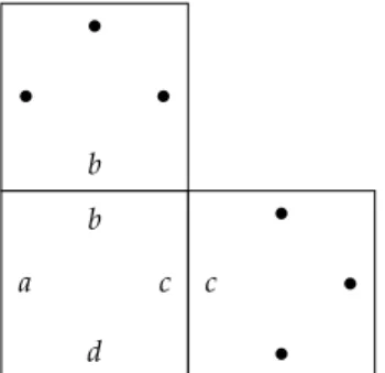
Definition 1.27. Adomino systemis a structureD= (D,H,V)with

• a finite setD,

• horizontal and vertical compatibility relationsH,V⊆D×D.

The meaning ofHandVis that

• (d,d^′)∈Hif the right colour ofdis equal to the left colour ofd^′,

• (d,d^′)∈Vif the top colour ofdis equal to the bottom colour ofd^′ (see Figure 1.1).

A tiling ofN×NbyDis a functionσ:N×N→Dsuch that for all x,y∈_N

• (_σ(x,y)_,_σ(x+_1,y))∈Hand

• (_σ(x,y)_,_σ(x,y+₁))∈V.

(20)

A periodic tiling ofN×NbyDis a tilingσfor which two integers h,v∈_Nexist such that for allx,y∈_Nit holdsσ(x,y) =σ(x+h,y) = σ(x,y+v). The decision problem DOMINO is described as

DOMINO :={D: there exists a tiling ofN×_NbyD}

a b

c d

c

•

• b

Figure 1.1.Domino adjacency condition

An important variant is the origin constrained tiling.

Definition 1.28. Anorigin constrained domino systemis a system(D,D₀) withD₀⊆D. A tiling with origin constraintD₀is a tilingσsuch that σ(0, 0)∈D0. The corresponding decision problem is

CORNER-DOMINO :={(D,D0): there exists a tiling ofN×_N with origin constraintD₀}. Theorem 1.29(Wang, Büchi). CORNER-DOMINO is undecidable.

Proof. We reduceH^ω_ε ={ρ(M): the computation ofMonεis infinite}, which is co-r.e., to CORNER-DOMINO.

Consider a 1-tape TMM= (Q,Σ,q₀,δ,F), and construct(D,D₀) such that the computation ofMonεis infinite if and only if there exists a tiling ofN×_NbyDwith origin constraintD₀.

Assume w.l.o.g. that Mnever moves off-tape to the left, i.e. in configurations(q, 0,w)it is never the case thatδ(q,w₀) = (q^′,a,−1)_.

16

(21)

1.3 Domino problems

Dconsists of the following domino types.

For eacha∈_Σ ↔

a

↔ a

For each(q,a)∈Q×_Σwith

δ(q,a) = (q^′,a^′, 0) ↔

(q^′,a^′)

↔ (q,a)

For each(q,a)∈Q×_Σwith δ(q,a) = (q^′,a^′, 1), for each b∈_Σ

↔ a^′

(q,a) (q,a)

(q,a) (q^′,b)

↔ b

For each(q,a)∈Q×_Σwith δ(q,a) = (q^′,a^′,−1)for each b∈_Σ

↔ (q^′,b)

(q,a) b

(q,a) a^′

↔ (q,a)

Additionally there exist

dominoes ⊢

(q₀,)

↔₀

⊥

↔₀

⊥

The origin constraintD₀con-

sists of ⊢

(q₀,)

↔₀

⊥ Note that(D,D₀)can be constructed effectively fromM.

There is precisely one way of tiling the first row:

(22)

⊢ (q₀,)

↔₀

⊥ σ(_{0, 0})

↔₀

⊥

σ(_0,i) _{for all}i>₀

· · ·

Assume the firstjrows have been tiled correctly. Then the top edge of rowjreads

w₀. . .wi−1(q,w_i)w_i+1. . .

forC_j= (q,i,w₀,w₁, . . .), thejth configuration ofMonε.

This tiling can be extended to a tiling of rowj+1 if and only if there existsC_j+1=Next(C_j).

Conclusion: The computation ofMonεis infinite if and only if there exists a tiling ofN×_Nby(D,D₀). q.e.d.

Stronger forms of this result are the following

Theorem 1.30(Berger, Robinson). DOMINO (without origin constraint) is co-r.e. and undecidable.

Theorem 1.31. The problem of tilingZ×_Zis reducible to the problem of tilingN×N. (Proof via König’s Lemma).

Theorem 1.32. The set of domino systems admitting a periodic tiling ofN×N, those that admit no tiling ofN×Nand those that admit a tiling but not a periodic one are pairwise recursively inseparable.

Definition 1.33. A computable function f is a reduction from domino systemstoXif, for all domino systemsD, f(D) =ϕD is inXand the following holds:

• Dadmits a periodic tiling ofN×_N⇒ψDhas a finite model

• Dadmits no tiling ofN×N⇒ψD is unsatisfiable

• Dadmits a tiling ofN×Nbut no periodic one⇒ψDis an infinity axiom.

18

(23)

1.4 Applications of the domino method

Remark 1.34. Let X ∈ FO. If there exists a reduction from domino systems toXthenXis a conservative reduction class.

Proof. SinceFin-sat(FO)andNon-sat(FO)are recursively enumerable andInf-axioms(_FO)is co-recursively enumerable, we can associate with every first-order formulaψa Turing machineMsuch that

• ψ∈Fin-sat(_FO)⇒ρ(M)∈H_ε⁺,

• ψ∈Non-sat(_FO)⇒ρ(_M)∈H_ε⁻,

• ψ∈Inf-axioms(FO)⇒ρ(M)∈H_ε^∞.

The proof of 1.32 reduces the halting problemsH_ε⁺,H_ε⁻,H^∞_ε , to the domino problems. There exists a recursive function that associates with every TMMa domino systemDsatisfying

• IfM∈H_ε⁺thenDadmits a periodic tiling ofN×_N.

• IfM∈H_ε⁻thenDadmits no tiling ofN×_N.

• IfM∈H_ε^∞thenDadmits a tiling ofN×_Nbut no periodic one.

Finally, according to to the assumption, there is a reduction D 7→

ϕ_D from domino systems to X Thus, the domino method yields a conservative reduction from FO toX.

q.e.d. 1.4 Applications of the domino method

We now apply the domino method to obtain several reduction classes.

Theorem 1.35. [∀∃∀,(0,ω),(0)]is a conservative reduction class.

Proof. Due to Remark 1.34 it suffices to give a reduction from domino systems toX, i.e. find a mappingD 7→ψD over a vocabulary consisting of binary relation symbols(P_d)_d∈D_{such that}

(1) Dadmits a periodic tiling ofN×_N⇒ψDhas a finite model (2) Dadmits no tiling ofN×_N⇒ψDis unsatisfiable

(3) Dadmits a tiling ofN×_Nbut no periodic one⇒ψDis an infinity axiom

(24)

The intended model isN with intended interpretation ofP_d = {(i,j)∈_N×_N:τ(i,j) =d}for alld∈D. We defineψDby

ψ_D :=∀x∃y∀z _^

d̸=d^′

P_dxz→ ¬P_d^′xz

∧ ^_

(d,d^′)∈H

(P_dxz∧P_d^′yz)∧ ^_

(d,d^′)∈V

(P_dzx∧P_d^′zy). ObviouslyψDis of the desired format, i.e.ψD∈[∀∃∀,(0,ω),(0)].

(1) IfDadmits a periodic tiling ofN×_{N, then}ψ_D has a finite model.

Letτ:N×_N→Dbe a periodic tiling such that for someh,v∈_N τ(x,y) =τ(x+h,y) =τ(x,y+v)for allx,y. Lett:=lcm(h,v)be the least common multiple ofhandv. Thenτinduces a tiling

τ:Z/tZ×_Z/tZ→D

withτ^′(x,y) =τ(x( modt),y( mod t)).

Thus,A= (_Z/tZ,(P_d)_d∈D)with P_d ={(i,j) : τ^′(i,j) = d}is a finite model (forxinψDchoosey:=x+1 (modt)inψD.) (2) IfψDhas a model, thenDadmits a tiling.

(3) We want to show: ifψDhas a finite model, thenDadmits a periodic tiling. (In the case thatψD is unsatisfiable, we show with the same arguments as in(1)that ifDadmits a tiling ofN×_{N, then}ψD

has a modelA= (_N,(P_d)_d∈D).)

Let nowψD have a finite model. To show that ifψDhas a (finite) model, thenDadmits a (periodic) tiling we consider the Skolem normal formϕDofψD:

ϕD :=∀x∀z(^{^}

d̸=d^′

P_dxz→ ¬P_d^′xz

∧ ^_

(d,d^′)∈H

(P_dxz∧P_d^′f xz)∧ ^_

(d,d^′)∈V

(P_dzx∧P_d^′z f x).

• SupposeB= (B,f,(P_d)_d∈D)|=ϕD. Define a tilingτ:N×_N→ D as follows: chooseb ∈ B, and setτ(i,j) _:= dfor the unique

20

(25)

d∈Dsuch thatB|=P_d(fⁱb,f^jb)_{for all}i,j∈N. SinceB|=_ϕ_D_,_τ is a correct tiling.

• Suppose thatB|=ϕD is finite:

• •

f b

f · · · •

f

Chooseb∈Bsuch that, for somet≥1, f^tb=b. Then the defined tilingτis periodic.

q.e.d. Corollary 1.36. FO³is a conservative reduction class.

Later we show thatFO²has the FMP.

Consider sets of formulaeX⊆FO over functional vocabularies.

FO(τ)is a conservative reduction class ifτcontains

• two unary functions or

• one binary function.

This is even true for sentences of the form∀xϕwhereϕis quantifier- free.

Theorem 1.37. [∀,(0),(2)]₌and[∀,(0),(0, 1)]₌are conservative reduction classes.

Proof. We apply the domino method for formulae ∀xϕ where ϕ is quantifier-free with any number of unary functions, and then apply a reduction/interpretation to reduce this to two unary/one binary function/s.

Define a mappingD = (D,H,V) 7→ ψD whereψD is a formula over the vocabulary {f,g,(h_d)_d∈D} where all function symbols are unary. The intended model isN×_Nwith successor functions f andg.

The subformula∀x(f gx=g f x)ensures that the models ofψD contain a two-dimensional grid. The fact that a positionxis tiled byd∈Dis

(26)

expressed by requiring thath_dx=x, i.e. thatxis a fixed point ofh_d. Now define

ψD:=∀x f gx=g f x∧ ^{^}

d̸=d^′

(h_dx=x→h_d^′x̸=x)

∧ ^_

(d,d^′)∈H

(h_dx=x∧h_d^′f x= f x)

∧ ^_

(d,d^′)∈V

(h_dx=x∧h_d^′gx=gx).

We claim that there exists a tilingσ:N×N→ Dif and only if ψD is satisfiable.

”⇒” Assumeσis a correct tiling. Construct the (intended) model A= (_N×_N,f,g,(h_d)_d∈D)with

– f(i,j) = (i+1,j), – g(i,j) = (i,j+1), – h_d(i,j)







= (i,j) ifσ(i,j) =d

̸= (i,j) otherwise.

ClearlyA|=ψD.

”⇐” ConsiderB= (B,f,g,(h_d)_d∈D)|=ψD. Choose an arbitraryb∈Band define

σ:N×_N→ D:σ(i,j):=diffB|=h_dfⁱg^jb= fⁱg^jb.

Note that every position is in exactly one of the h_d. Thenσis a correct tiling. If Bis finite, then σis periodic, and thus the reduction is conservative.

We now show that we can sharpen the results, i.e. show that two unary function symbols are sufficient

Consider∀xϕ∈[∀,(0),(ω)]₌ with monadic function symbols f₁, . . . ,fm. Transform ϕinto ˜ϕ:=ϕ[x/hx,f_i/hgⁱ]whereh,gare fresh unary function symbols. This procedure transforms formulae over the vocabulary{f₁, . . . ,fm}into formulae over the vocabulary{h,g}. The idea is to replace an application off_ibyiapplications ofg. The second functionhtakes care of unwanted equalities.

22

(27)

1.4 Applications of the domino method x

• • · · · •

f₁ f₂ fm

x

hx

• • · · · • •

g^m(hx) h

g

g g

Claim:∀xϕis (finitely) satisfiable⇔ ∀xϕ˜ is (finitely) satisfiable.

”⇐” LetB= (B,h,g)|=∀xϕ. Construct˜ A= (A,f₁, . . . ,fm)with – A={hb:b∈B}

– f_i(a) = (hgⁱ)(a) ThenA|=∀xϕ.

”⇒” LetA= (A,f₁, . . . ,fm)|=∀xϕ. ConstructB= (B,g,h)with – B=A× _Z/(m+1)_Z,

– g(a,i) = (a,i+1), – h(a, 0) = (a, 0), – h(a,i) = (fia, 0).

This transformation preserves the meaning of terms: Lett(x) = f_i₁. . .f_i_kxbe a term inϕ. Then ˜t(x) =hgⁱ¹. . .hgⁱ^khx, and it holds that ˜t^B[a, 0] = (t^A[a], 0). Now the claim follows via induction over the structure ofϕ.

We now show that we need at most one binary function. The idea is to find an interpretation of g,h: A→Ain a structureA= (A,F) withF:A×A→Avia

• g(a) =F(a,F(a,a)),

• h(a) =F(F(a,a)_,a)

(28)

whereF(a,a)̸=a.

Formally, consider a formula∀xϕwith unary function symbols f,g. Introduce a new binary function symbolFand translate

ϕ7→ϕg∧ϕ_h where

ϕg:=ϕ[x/g^∗x,g/g^∗,h/h^∗], ϕ_h:=ϕ[x/h^∗x,g/g^∗,h/h^∗] with

g^∗t=F(t,Ftt), h^∗t=F(Ftt,t).

Claim: ∀xϕ(finitely) satisfiable ⇔ ∀x(ϕg∧ϕ_h) (finitely) satisfiable.

”⇒” LetA= (A,g,h)|=∀xϕbe a model. SetB= (B,F)with – B:=A×_Z/3Z

– F((a,i),(a,i)):= (a,i+1) – F((a,i),(a,i+1)):= (ga, 0) – F((a,i+1),(a,i)):= (ha, 0). Now, for all(a,i)∈B

g^∗(a,i) =F (a,i),F(a,i)(a,i)=F (a,i),(a,i+1)= (ga, 0) and

h^∗(_a,_i) = (_{ha, 0})_.

ThusAis isomorphic to a copy ofAdefined inB.

A∼=A^∗:= ({(a, 0)_:a∈A},g^∗,h^∗)_. Therefore, for all(a,i)

B|=_ϕ_g(a,i)⇔A^∗|=_ϕ(ga, 0)

24

(29)

⇔A |=ϕ(ga) and B|=ϕ_h(a,i)⇔A^∗|=ϕ(ha, 0)

⇔A |=ϕ(ha).

Thus,A|=∀xϕimpliesB|=∀x(ϕg∧ϕ_k).

”⇐” ForB= (B,F)|=∀x(ϕg∧ϕ_h)letA= (A,g,h)with – A:=g^∗(B)∪h^∗(B)

– g:=g^∗ – h:=_h^∗

ThenA|=∀xϕ. q.e.d.

(30)

(31)

2 Finite Model Property

We study the finite model property for fragments of FO as a mean to show that these fragments are decidable, and also to better understand their expressive power and algorithmic complexity.

Recall that a classX⊆FO has thefinite model propertyifSat(X) = Fin-sat(X). Since for any decidable classX,Fin-sat(X)is r.e. andSat(X) is co-r.e., it follows thatSat(X)is decidable ifXhas the FMP. In many cases, the proof that a class has the finite model property provides a bound on the model’s cardinality, and thus a complexity bound for the satisfiability problem. To prove completeness for complexity classes we make use of a bounded variant of the domino problem.

2.1 Ehrenfeucht-Fraïssé Games

2.1.1 Atomic Types

Definition 2.1. Theatomic k-typeofa₁, . . . ,a_kinAis defined as atp_A(a₁, . . . ,a_k):={γ(x₁. . . ,x_k):γatomic formula or negated

atomic formula such thatA|=γ(a₁, . . . ,a_k)}. We assume that all structures contain unary or binary relations only.

Hence, to describe a structure it suffices to define its universe and to specify the atomic 1-types and 2-types for all of its elements.

Example2.2. Let Abe the structure(A,E₁, . . . ,Em) where the E_i are binary relations. Then fora∈A:

atp_A(a) ={E_ixx:A|=E_iaa} ∪ {¬E_ixx:A|=¬E_iaa}.

Definition 2.3. LetAandBbe structures over the same signature and

(32)

2 Finite Model Property

a⊆ Aandb⊆ B. We say thatA,ais locally isomorphic toB,band writeA,a≡₀B,bifahas the same atomic type inAasbinB.

2.1.2 The Game EFm(A,B)

The Ehrenfeucht-Fraïssé game EFm(A,B) is played by two players according to the following rules.

The arenaconsists of the structuresA andB. We assume that A∩B=∅. The players are calledSpoilerandDuplicator, and a play of EFm(A,B)consists ofmmoves.

In the i-th move, Spoiler chooses either an element a_i ∈ Aor an elementb_i∈B. Duplicator answers by choosing an element in the other structure.

Afterm moves, elements a₁, . . . ,a_m fromAand b₁, . . . ,b_m from B are chosen. Duplicator wins the play if A,(a₁,a₂, . . . ,am) ≡₀ B,(b₁,b2, . . . ,bm). Otherwise Spoiler wins.

Afterimoves inEFm(A,B)are made, a position(a₁, . . . ,a_i,b₁, . . . ,b_i) is reached. We denote the remaining subgame in whichm−imoves are left byEFm−i(A,a₁, . . . ,a_i,B,b₁, . . . ,b_i).

A winning strategyof Spoiler for such a subgame is a function which, for every reachable position, determines a move such that Spoiler wins each play which is consistent with this strategy, no matter how Duplicator plays. Winning strategies for Duplicator are defined analogously.

We say thatSpoiler (respectively, Duplicator) wins the game EFm(A,B) if this player has a winning strategy forEFm(A,B). By induction on the number of moves it is easy to show that for every (sub)game exactly one of the two players has a winning strategy.

Example2.4.

• LetA= (Z,<),B= (R,<). Then Duplicator winsEF2(A,B), but Spoiler winsEF₃(A,B).

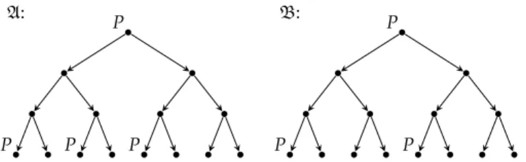
• For a relational signatureτ={E,P}(wherePhas arity one and Ehas arity two), consider the structuresAand Bin Figure 2.1.

Spoiler wins the gameEF₃(A,B), but Duplicator winsEF₂(A,B).

28

(33)

2.1 Ehrenfeucht-Fraïssé Games A:

P P P

P B:

P P

P

Figure 2.1. Two structuresAandBwithA≡₂BandA̸≡₃B

2.1.3 The Game EF(A,B)

An important variant is the Ehrenfeucht-Fraïssé game EF(A,B) in which plays of arbitrary length are possible. In each play, Spoiler first chooses anm∈N, and then the players play the gameEFm(A,B).

Spoiler wins the gameEF(A,B)if and only if there exists anm∈_N such that he wins the game EF_m(_A,B). In other words: Duplicator winsEF(A,B)if and only if she has a winning strategy for each of the gamesEFm(A,B).

Recall that two structuresAandBare said to beelementarily m- equivalent, writtenA≡_mB, if no first-order formula of quantifier rank at mostmcan separate both structures. IfA≡_mBfor allm∈_Nwe write A≡Band say thatAandBareelementarily equivalent. The following theorem shows that elementary equivalence and Ehrenfeucht-Fraïssé games are in some sense equivalent concepts.

Theorem 2.5(Ehrenfeucht, Fraïssé). Letτbe finite and relational, and letA,Bbeτ-structures.

(1) The following statements are equivalent:

(i) A≡B.

(ii) Duplicator wins the Ehrenfeucht-Fraïssé gameEF(A,B). (2) For allm∈Nthe following statements are equivalent:

(i) A≡_mB.

(ii) Duplicator winsEFm(A,B).

In fact, even the following, somewhat stronger proposition holds (for a proof see the lecture notes of mathematical logic).

(34)

Theorem 2.6. Let A,B be τ-structures, ¯a = a₁, . . . ,a_r ∈ A, ¯b = b₁, . . . ,br ∈ B. If there exists a formulaψ(x¯) with qr(ψ) = m such thatA |= ψ(a¯) and B |= ¬ψ(b^¯) holds, then Spoiler has a winning strategy for the gameG_m(A, ¯a,B, ¯b).

We use the above to prove finite model property of the following fragment of FO.

Theorem 2.7. Ifτcontains only unary predicates then FO[τ]has FMP.

Proof. LetA= (A,P1, . . . ,Pn)and let qr(ϕ) =m. For each sequence of bitsα=α₁. . .αnwe defineP_α=Q₁∩Q₂∩. . .∩Qn, whereQ_i=P_iif α_i=1 andQ_iis the complement ofP_ielse.

Note that {α | x ∈ P_α} determines all atomic types of x. We constructBby taking min(|P_α|,m)elements into each P_α^B. Observe thatBis defined in this way (takeP_i^B=^S_α|α_i₌₁P_α^B). We show that A≡_mBusing the Ehrenfeucht-Fraïssé Theorem.

The following is a winning strategy for Duplicator in EF(A,B): Answer each Spoiler’s choice of an element with an element of the same atomic type in the other structure. Due to the construction it is possible to do that formmoves. It also follows from the construction that≡₀is never violated and Duplicator wins the game. q.e.d.

You can see from the proof that the constructed finite modelBis a sub-model ofA. It is not always the case, sometimes it is not possible to find a finite sub-model, even for fragments with FMP.

2.2 FMP of Modal Logic

We proceed with proving that propositional modal logic (ML), which is an important fragment of FO², has the finite model property. In fact we establish an even stronger result showing that every satisfiable ML-formula has a finite model that is a tree. Hence, we prove that ML has thefinite tree model property.

30

(35)

2.2.1 Modal Logic

Let us first briefly review the syntax and semantics of propositional modal logic (ML).

Definition 2.8. For a given set of actions Aand atomic properties {P_i:i∈I}, the syntax of ML is inductively defined as:

• All propositional logic formulae with propositional variablesP_iare in ML.

• Ifψ,ϕ∈ML, then also¬ψ,(ψ∧ϕ)and(ψ∨ϕ)∈ML.

• Ifψ∈ML anda∈A, then⟨a⟩ψand[a]ψ∈ML.

Remark2.9. If there is only one actiona ∈ A, we write ♦ψand ψ instead of⟨a⟩ψand[a]ψ, respectively.

Definition 2.10. Atransition systemorKripke structurewith actions from a setAand atomic properties{P_i:i∈I}is a structure

K= (V,(Ea)_a∈A,(P_i)_i∈I)

with a universeV of states, binary relationsEa ⊆V×Vdescribing transitions between the states, and unary relationsP_i ⊆Vdescribing the atomic properties of states.

A transition system can be seen as a labelled graph where the nodes are the states ofK, the unary relations are labels of the states, and the binary transition relations are the labelled edges.

Definition 2.11. Let K= (V,(Ea)_a∈A,(P_i)_i∈I)be a transition system, ψ∈ML a formula andva state ofK. Themodel relationshipK,v|=ψ, i.e.ψholds at statevofK, is inductively defined:

• K,v|=P_iif and only ifv∈P_i.

• K,v|=¬ψif and only ifK,v̸|=_ψ.

• K,v|=ψ∨ϕif and only ifK,v|=ψorK,v|=ϕ.

• K,v|=ψ∧ϕif and only ifK,v|=ψandK,v|=ϕ.

• K,v|=⟨a⟩ψif and only if there existswsuch that(v,w)∈E_aand K,w|=ψ.

• K,v|= [a]ψif and only ifK,w|=ψholds for allwwith(v,w)∈Ea.

(36)

Definition 2.12. For a transition systemKand a formulaψwe define theextension

JψK

K:={v:K,v|=ψ}

as the set of states ofKwhereψholds.

2.2.2 Bisimulation

One of the most important notions in the analysis of modal logics is bisimulation. In fact bisimulation is closely related to logical equivalence of Kripke structures with respect to formulae from ML.

Definition 2.13. LetK= (V,(Ea)_a∈A,(P_i)_i∈I)andK^′= (V^′,(E_a^′)_a∈A,(P_i^′)_i∈I) be transition systems. AbisimulationbetweenKandK^′is a relation Z⊆V×V^′such that for all(v,v^′)∈Z

(Pred) v∈P_iif and only ifv^′∈P_i^′for alli∈I,

(Forth)for alla∈ A, w∈Vwithv−→^a wthere exists aw^′ ∈V^′with v^′−→^a w^′and it is(w,w^′)∈Z,

(Back)for alla∈A, w^′∈V^′withv^′−→^a w^′there exists aw∈Vwith v−→^a wand it is(w,w^′)∈Z.

Example2.14.

r r

✠ r

❅

w₁ ❘ w₂

v

Q Q

P

r ✲r ✲r

u^′ v^′ w^′

P Q

Z={(v,v^′),(w₁,w^′),(w₂,w^′)}is a bisimulation.

Definition 2.15. LetK,K^′be Kripke structures and letu∈V, u^′∈V^′. (K,u)and(K^′,u^′)arebisimilar(for short,K,u∼ K^′,u^′), if there exists a bisimulationZbetweenKandK^′such that(u,u^′)∈Z.

2.2.3 Bisimulation Invariance of Formulae of Modal Logic

The fundamental importance of bisimulation origins in the fact that formulae of modal logic are not able to distinguish between bisimilar

32

(37)

states. A more refined analysis considers the modal depth of formulae, i.e. the maximal depth of nesting of modal operators in a formula.

Definition 2.16. Themodal depthof a formulaψ∈ML is defined inductively by

(1) md(ψ) =0 for propositional formulaeψ, (2) md(¬_ψ) =md(_ψ),

(3) md(ψ◦ϕ) =max(md(ψ), md(ϕ))for◦ ∈ {∧,∨,→}, (4) md(⟨a⟩ψ) =md([a]ψ) =md(ψ) +1.

Definition 2.17. LetKand K^′ be two Kripke structures and letv∈ K, v^′∈ K^′.

(1) K,v≡_ML K^′,v^′if for allψ∈ML we haveK,v|=ψif and only if K^′,v^′|=ψ.

(2) K,v≡ⁿ_MLK^′,v^′if for allψ∈ML with md(_ψ)≤nwe haveK,v|= ψif and only ifK^′,v^′|=ψ.

One can refine the definition of the bisimilarity relation between transition systems as well. We say that(K,u)and(K^′,u^′)aren-bisimilar (for short,K,u∼_nK^′,u^′), if there exists a relationZbetweenKandK^′ such that(u,u^′)∈ZandZhas the property ’Pred’ and the ’Forth’ and

’Back’ property for all pairs of nodes(v,v^′)∈Zwith distance at mostn from(u,u^′). For a formal (game theoretical) definition, see the lectures notes of mathematical logic.

Theorem 2.18. For Kripke structuresK, K^′ andu ∈ K, u^′ ∈ K^′ the following holds:

(1) K,u∼ K^′,u^′ ⇒ K,u≡_MLK^′,u^′. (2) K,u∼_nK^′,u^′⇒ K,u≡ⁿ_MLK^′,u^′.

Statement (1) is called thebisimulation invariance of modal logic:

IfK,v|=ψandK,v∼ K^′,v^′, thenK^′,v^′|=ψ.

The reverse only holds for finitely branching systems. A transition system is finitely branchingif for all statesvand all actions athe set vEa:={w:(v,w) ∈Ea}ofa-successors ofvis finite. (for proofs see the lecture notes of mathematical logic).

Algorithmic Model Theory SS 2010