Policy Research Working Paper 7221
The Misallocation of Land and Other Factors of Production in India
Gilles Duranton Ejaz Ghani Arti Grover Goswami
William Kerr
Macroeconomics and Fiscal Management Global Practice Group March 2015
WPS7221
Public Disclosure AuthorizedPublic Disclosure AuthorizedPublic Disclosure AuthorizedPublic Disclosure Authorized
Produced by the Research Support Team
Abstract
The Policy Research Working Paper Series disseminates the findings of work in progress to encourage the exchange of ideas about development issues. An objective of the series is to get the findings out quickly, even if the presentations are less than fully polished. The papers carry the names of the authors and should be cited accordingly. The findings, interpretations, and conclusions expressed in this paper are entirely those of the authors. They do not necessarily represent the views of the International Bank for Reconstruction and Development/World Bank and its affiliated organizations, or those of the Executive Directors of the World Bank or the governments they represent.
Policy Research Working Paper 7221
This paper is a product of the Macroeconomics and Fiscal Management Global Practice Group. It is part of a larger effort by the World Bank to provide open access to its research and make a contribution to development policy discussions around the world. Policy Research Working Papers are also posted on the Web at http://econ.worldbank.org. The authors may be contacted at Eghani@worldbank.org, duranton@wharton.upenn.edu, artigrover@gmail.com, and wkerr@hbs.edu.
This paper quantifies the misallocation of manufacturing output and factors of production between establishments across Indian districts during 1989–2010. It first distills a number of stylized facts about misallocation in India, and demonstrates the validity of misallocation metrics by connecting them to regulatory changes in India that affected real property. With this background, the study
next quantifies the implications and determinants of factor and output misallocation. Although more-produc- tive establishments in India tend to produce more output, factors of production are grossly misallocated. A better allocation of output and factors of production is associ- ated with greater output per worker. Misallocation of land plays a particularly important role in these challenges.
The Misallocation of Land and Other Factors of Production in India
Gilles Duranton
Wharton School, University of Pennsylvania Ejaz Ghani
World Bank Arti Grover Goswami
World Bank William Kerr Harvard Business School
Acknowledgements: Financial support from the World Bank and CEPR Private Enterprise Development in Low-Income Countries programme is gratefully acknowledged. We appreciate the comments and guidance from Ed Glaeser, Vijay Jagannathan, Somik Lall, Jevgenijs Steinbuks, and conference and seminar participants. We are also grateful to Yoichiro Kimura for helping us to understand the repeal of ULCRA and sharing his data with us. The views expressed here are those of the authors and not of any institution they may be associated with.
2 1. Introduction
We study the misallocation of land and buildings inputs and other factors of production for the Indian manufacturing sector. Our paper makes four contributions. We first document that factor misallocation among establishments is substantially worse than that of output, and that districts vary substantially in the efficiency with which factors are allocated to the most productive establishments. Second, we validate these indices for studying land and building misallocation by showing their close connection to local policy and tax reforms in property markets. Building from these baselines, our third contribution is to demonstrate how land and building misallocation fosters the misallocation of output in local areas, in both the current context and also looking forward. We also show a strong connection of land and building misallocation to reduced labor productivity for districts.
The economic magnitudes of our results are substantial and provide an important lens for considering how to best foster economic development. Economists and policy makers have traditionally sought to encourage development and growth through increasing factor productivity and fostering factor accumulation. We show that a better factor allocation across establishments would also generate very large economic gains. We quantify that a one standard deviation decrease in the misallocation of land and buildings is associated with about a 25% increase in output per worker. This is equivalent to a six-fold increase in the land supply for manufacturing establishments in these districts. We also observe that the misallocation of other inputs to firms hampers performance, but land and building access appears especially important in India. This parallels accounts in the press of the exceptional and stifling nature of Indian land markets.
These insights provide an important input to the achievement of economic growth and the World Bank’s twin goals of reducing extreme poverty and promoting shared prosperity.
Our paper provides three distinct contributions to the academic literature. First, as we discuss below, there have been many studies arguing the importance of misallocation. The consequences of misallocation are usually inferred indirectly by asking a model what would be the aggregate consequences of reduced misallocation. That is, extant claims about the importance of misallocation rely on measures of aggregate misallocation and computations of counterfactuals
3
from particular models. In contrast, we provide direct evidence about the importance of misallocation by investigating empirically the link between factor misallocation across establishments and output per worker, using subnational regions in cross-section and in panel.
Second, increasing the productivity of factors of production, fostering their accumulation, and reducing their misallocation can only be viewed as proximate causes of economic growth and development. Importantly, as part of our metric validation, we begin to make connections between policies and factor misallocation. Our findings suggest that factor misallocation is not exogenously determined but is instead affected by policies. More generally, we think of our results as emphasizing the importance of “frictions” as key determinant of the efficiency of factor allocation and, in turn, prosperity. Policies can be a source of friction. Better policies can also reduce frictions and improve allocation. Our emphasis on frictions differs from many models in the literature that rely on idiosyncratic distortions as the root cause of misallocation.
Third, we highlight the uniquely important role played by land and buildings in misallocation.
We attribute this to the fact that choosing a location is a decision that conditions many others and cannot easily be changed, especially in an environment with poorly functioning land markets.
More productive establishments will have a tough time buying more machines or employing more workers if they have no room to accommodate them. Land may also be a uniquely important asset for establishments that seek to expand since it can be used as collateral for external financing. While we do not take a stance regarding the exact mechanism through which land and buildings affect factor misallocation, our results highlight that land used for non- agricultural production may play a more important role than hitherto thought. Better land policies can make land more broadly available and reduce the frictions associated with land transactions.
We are nonetheless aware that the elimination of frictions on the land market would require more than better land use regulations and a more efficient taxation of properties. Better-functioning land markets also require clearly defined property rights, a reliable land registry, and a number of other institutional improvements. This is a considerable challenge in a country like India where property rights for land and buildings are poorly defined and often conflict with tenancy rights.
4
To conduct our study, two main challenges need to be overcome. The first is to develop a methodology that allows us to explore the effects of misallocation and its determinants in a cross-section of districts. To do this, we develop indices of misallocation in the spirit of the decomposition originally proposed by Olley and Pakes (1996). In essence, misallocation can be measured by the difference between un-weighted mean establishment productivity and mean establishment productivity weighted, typically, by output. This difference is proportional to the covariance between establishment productivity and output. A higher covariance indicates a more efficient allocation as more productive establishments produce more output.
Our analysis starts with two simple observations. First, Olley-Pakes misallocation indices can be computed not only for output but also for each factor of production separately. Second, these misallocation indices need not be computed exclusively at the country level. They can also be produced for subnational units such as districts. Interestingly, there is a lot of variation in misallocation across the different misallocation indices and for each index across districts. We then think about misallocation as an intermediate outcome which we can relate to final outcomes of interests such as output per worker (or establishment productivity). We can also relate these intermediate misallocation outcomes to deeper causes such as policies or the local characteristics of districts.
More specifically, our analysis proceeds in five steps. The first is to estimate the productivity of all establishments in the data and factor shares for all industries. Establishment productivity is a necessary input to measure misallocation, and we consider several approaches to estimating productivity. Our second step is to compute misallocation indices for output and for each factor of production at the district level. The main difficulty here is that misallocation is most meaningfully computed at the industry level since industries differ in their factor intensity.
Measures of misallocation at the district-industry level must thus be aggregated across industries to obtain a district-level measure. After distilling some stylized facts about misallocation across districts, our third step validates these metrics for studying land and building access by showing a connection of them to unanticipated local policy reforms that affect property markets.
5
In the fourth step, we quantify the relationship between various forms of misallocation. This step allows us to tease out the unique role played by the misallocation of land and buildings among Indian establishments. This misallocation of land and buildings is at the root of much of the misallocation of output. The last step examines the effects of factor misallocation on establishment productivity and output per worker. This analysis affords statements about which forms of misallocation matters more in Indian districts. Again, land and buildings appear especially important given their relatively small cost share.
The second main challenge is one of data. To compute measures of misallocation at the district level, establishment/plant data are needed as large firms may be present in many districts.
Although it is always possible to apportion consolidated firm-level accounts across their various establishments, it is easier and more accurate to exploit establishment-level information. Our analysis is also best conducted using detailed information about the balance sheets of establishments to distinguish between different types of fixed factors. Although our approach can be applied to more aggregated factors (e.g., all fixed inputs), some of our more interesting findings come from our ability to distinguish more finely across different forms of capital, such as land and building vs. other fixed assets. Our analysis also requires a large country with enough subnational units to exploit sufficient cross-sectional information. Each subnational unit also need to be large enough for our measures of misallocation to carry some information and not be driven only by sample variation. Sampling issues are all the more important since our indices of misallocation must be first calculated at the level of each sector and district and then aggregated across sectors within each district. Finally, our country of study should be heterogeneous enough for there to be sufficient variation in misallocation.
India is well suited for our purpose. The government conducts regular censuses of production at the establishment level and requires establishments to report their assets with an unusual level of detail. India is also an extremely large country composed of several hundred districts, most of which contain enough establishments for us to compute informative measures of misallocation.
Although we discuss our methodology and findings in relation to the literature in greater detail below, we note that our work mainly contributes to the misallocation literature recently pushed
6
forward by the seminal contributions of Restuccia and Rogerson (2008) and Hsieh and Klenow (2009). As already mentioned we explicitly measure how factor misallocation affects output per worker using a cross-section of subnational units rather than infer it indirectly from a model. We also show how factor misallocation affects output misallocation. Finally, we provide evidence regarding the effects of some economic policies on factor allocation.
2. Background and data
Our analysis considers five surveys from two major sources of data: the Annual Survey of Industries (ASI) and National Sample Survey Organization (NSSO). These data have been used extensively in prior research on the Indian economy, including Ghani et al. (2014) from which the first part of this data description builds on. ASI is a survey of the organized sector undertaken annually by the Central Statistical Organization, a department in the Ministry of Statistics and Program Implementation of the Government of India. Under the Indian Factory Act of 1948, all establishments employing more than 20 workers without using power or 10 employees using power are required to be registered with the Chief Inspector of Factories in each state. This register is used as the sampling frame for the ASI. The ASI extends to the entire country, except the states of Arunachal Pradesh, Mizoram, and Sikkim and Union Territory (UT) of Lakshadweep.
The ASI is the principal source of industrial statistics for the organized manufacturing sector in India. It provides statistical information to assess changes in the growth, composition, and structure of organized manufacturing sector comprising activities related to manufacturing processes, repair services, gas and water supply, and cold storage. As noted in Ghani et al.
(2012b), organized manufacturing contributes a substantial majority of India’s manufacturing output, while the unorganized sector accounts for a large majority of employment for Indian manufacturing workers. Manufacturing activity undertaken in the unorganized sector, such as households (own-account manufacturing enterprise) and unregistered workshops, is covered by the NSSO. The distinction between the organized and unorganized sectors broadly captures the difference between formal and informal sectors.
7
Our study considers data taken from 1989-90, 1994-95, 2000-01, 2005-06, and 2010-11. In the first four instances, we use contemporaneous ASI and NSSO surveys. In the last period, we use 2009-10 ASI data and 2010-11 NSSO data. For simplicity, we normally refer to a sample survey by its starting year—for example, the sample survey in the year 2005-06 is referred to as the 2005 survey. We use 2010 in the tables and text to refer to the years 2009-10 for ASI data and years 2010-11 for NSSO data.
Establishments in both the organized and unorganized sectors provide information on the value of the land and buildings that they own. Although both sectors provide this information, only the organized sector surveys offer the distinction across land and buildings consistently for all the survey years under consideration.1 For the unorganized sector, this separation between land and buildings stops in 2000. Thus, in this sector, we always consider land and buildings together.
Some businesses rent the land that they operate on. The questionnaires for both sectors ask renting establishments to provide information on the rent paid for land and buildings. The NSSO goes a step further and requires establishments report the value of the land and buildings that they rent. The organized sector survey also provides information on the rent paid and/or received for land and buildings for the years 2000, 2005, and 2010. To impute the value of land and buildings rented by establishments, we use the reported values for the land and buildings when available. Otherwise, our imputations use rents and estimated local capitalization rates as described in appendix box 1. Appendix tables 1a and 1b provide details and exact wording of the questions pertaining to land and building values that appear in the respective survey questionnaires. In robustness checks, we duplicate our main regressions for the samples of only owners and only renters and find similar results.
The raw data from the five survey years contain 262,911 observations in the organized sector and 955,234 observations in the unorganized sector. In the organized sector, we retain establishments whose status is declared to be open, thereby dropping establishments that were closed during the
1 The survey provides data on opening value, closing value, gross value, depreciation and so on for land and buildings. Closing net value of land and buildings is taken as the value of land and buildings owned. To obtain the value of the total land and buildings owned by establishments in the organised sector, we simply sum the separate values of land and buildings.
8
reference year, non-operational, deleted due to deregistration, or out of coverage (that is belonging to defense, oil storage, etc.). This step leaves 216,898 observations in the organized sector. Next, we drop establishments that do not belong to the manufacturing sector. Such industries may relate to mining and quarrying, fishing and aquaculture, or services sectors (e.g., electricity; water supply; transportation; wholesale/retail trade). This pruning yields a sample count of 203,031 for the organized sector and 655,571 for the unorganized sector. Finally, we delete observations with missing, null, negative, or extremely large values of output (being greater than 1 billion rupees), output per worker (being null or greater than 1 million rupees), or employment (being over 500,000). At this stage, we also delete from the NSSO surveys the states that are not surveyed by ASI. We also delete observations that have blank state codes.
These exclusions result in a sample of 169,814 observations for the organized sector and 651,808 for the unorganized sector.
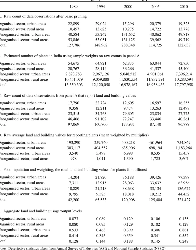
Table 1 reports a number of descriptive statistics about the data we use and its coverage. Panel A provides a raw count of observations after basic pruning for each type of establishment and year of data. Panel B reports the corresponding number of establishments in Indian manufacturing.
Panel C contains the number of establishments that report the value of land and buildings owned, while panel D reports average values of land and buildings owned by establishments in Indian manufacturing after winsorization at the 1% level. Panel E contains some information about post imputation values and the transformation of rental values into asset values.
Finally, panel F reports the revenue shares of land and building for various subsets of Indian manufacturing establishments and years of data. As these trends are of interest in their own right, Ghani et al. (2014) provides additional tabulations and notes on how these trends compare to that of energy usage, the primary subject of Ghani et al. (2014). Two key results are worth noting here. First, the early stability of land and building usage per output unit and its rise in 2010 are consistently observed when preparing the data with alternative procedures. Second, a decomposition exercise finds that almost all of the increase in land and building intensity is occurring within districts, rather than being due to reallocation of activity over districts (e.g., establishments moving toward high-priced areas). This within-district feature motivates the emphasis in this paper on district-level analyses.
9
To estimate productivity and misallocation, we need to further clean up the data by dropping establishments with negative value added, missing raw materials value, unknown district names, and/or locations in small and conflict states. These include Andaman and Nicobar Islands, Dadra
& Nagar Haveli, Daman & Diu, Jammu & Kashmir, Tripura, Manipur, Meghalaya, Mizoram, Nagaland and Assam. The final sample that we work with for productivity and misallocation metrics consists of 145,829 observations from the organized sector and 575,989 observations from the unorganized sector. This leaves us with over 320 districts each year for the two sectors, and appendix table 2 provides exact counts for each sector and year. These numbers roughly correspond to the number of districts for which land and building values are available. Although we end up considering only about half of the 630 Indian districts in our study, the included districts represent over 95% of establishments, employment, and output in the manufacturing sector throughout the study period.2
3. Measuring misallocation
3.1 Output and factor misallocation
Firms differ enormously in what they produce and how they produce it. Even within narrowly defined market segments, firms are very heterogeneous in how productive they are (Fox and Smeets, 2011; Syverson, 2011). For example, a firm at the top decile of productivity is twice as productive as a firm in the bottom decile for a typical manufacturing industry in the United States (Syverson, 2011). For India and China, a firm at the top productivity decile may be five times as productive as a firm at the bottom decile (Hsieh and Klenow, 2009).
A distribution of firm productivity within a given industry, however narrowly defined, is not necessarily a sign of inefficiency. Managers of the most productive firms may not be able to supervise all the workers in the industry (Lucas, 1978). Some poorly productive firms may also produce some highly specific varieties that some consumers value (Melitz, 2003). High transport
2 Our analyses also use a number of social, economic and geographic characteristics of districts as well as information about specific policies. We describe these data as they are introduced.
10
costs may also lead to less productive firms serving customers in remote areas. At the same time, a number of features may prevent firms from operating efficiently. So far the literature has focused mainly on idiosyncratic taxes on inputs and outputs faced by firms (Restuccia and Rogerson, 2008; Hsieh and Klenow, 2009) experiencing financial market frictions (Banerjee and Moll, 2010; Midrigan and Xu, 2014) and poor management (Bloom et al., 2013).
This said, most models of heterogeneous firms predict that more productive firms should be producing more output and using more factors of production. More specifically, these models imply that the most productive firms should be the ones with the highest revenue and should also be using the largest amounts of factors of production. It is easy to understand that if a more productive firm uses a smaller amount of land, less capital, and fewer workers than a less productive firm, total output would increase by reallocating some amount of these factors of production from the less to the more productive firm. Then, from this, it follows that the ranking of firms by productivity should be the same as the ranking of firms by factor usage. Productivity and factor usage should be perfectly (rank-)correlated under a perfectly efficient allocation of factors across firms.
Thus, a less than perfect correlation between productivity and factor usage indicates a misallocation of factors across firms. The worse the correlation between productivity and factor usage, the more misallocated are factors of production and the less output is produced relative to an efficient allocation. Using this insight, Olley and Pakes (1996) propose to measure misallocation using the covariance between firm productivity and output. Box 1 provides some technical details. This measure of allocation is also equal to the difference between un-weighted and weighted productivity, where the weights are the firm shares of output. The Olley-Pakes (OP) measure of misallocation—sometimes referred to as the OP decomposition—has been widely used to explore issues such as changes in factor allocation in the telecom industry after deregulation (Olley and Pakes, 1996), the effects of structural reforms in developing countries (Eslava et al., 2006), productivity differences across countries (Bartelsman et al., 2013), and the role financial institutions in factor allocation (Midrigan and Xu, 2014).
11
12
Relative to extant literature, we expand the OP approach in two directions. First, as already noted, while the literature computes misallocation indices using output or value added, analogue misallocation indices can be computed through weighting establishments by their use of any given factor of production instead of output. More formally, depending on what is used to measure establishment share, we can build measures of allocation efficiency for output, value added, employment, land, land and buildings, etc. This variety of measures allows us to explore
13
how various measures of allocation efficiency are related to each other and which ones matter to determine aggregate outcomes.
Second, we compute misallocation indices for subnational units. At this point it is important to clarify what a measure of misallocation within a district captures. Computing the misallocation of, say, employment in each district separately yields a measure of the misallocation of workers within each district, taking as given the distribution of employment across districts. Hence, the misallocation of employment within districts is only one component of the misallocation of employment in the entire country. For instance, it is possible to imagine situations where more productive establishments employ more workers within each district, but that districts that host more productive establishments on average have access to substantially fewer workers than less productive districts. This would be a case of a low level of misallocation within districts but a high level of misallocation across districts. While we leave the analysis of misallocation across districts for ongoing work as described in the conclusions, we note that our focus on within- district misallocation is warranted by the fact that within- and between-district misallocations probably have very different root causes and most likely call for different policies.
3.2 Issues with measuring misallocation at the district level
Our primary metrics of misallocation focus on the combined organized and unorganized manufacturing sectors, and we also directly compute the misallocation within each sector. We compute indices of misallocation for output, value added, and factors of production taken individually, such as employment, or in subsets, such as land and buildings or all fixed assets.
We then use these measures of misallocation across Indian districts in various regressions that seek to validate their usefulness and describe the implications of factor misallocation.
Leaving aside for now the issues associated with the specifics of our regressions, our approach raises two broad concerns. The first is that the measures of misallocation that we use, while intuitive and informative, are not structural. Below, we compare the estimates obtained from our regressions to counterfactuals from the models used in the literature so far, typically finding quite consistent results.
14
The second main issue is that our approach requires measures of misallocation at the district level, while the OP approach generates measures of misallocation within industries. To reconcile this requirement of a district-level misallocation measure with industry-level measures, the most obvious solution is to compute misallocation at the industry level within each district and then aggregate across industries within each district.
Aggregating industry-level indices of misallocation within each district to obtain a district index of misallocation can be performed in several ways. Our baseline computation sums industry misallocation across all industries and weights each industry by its corresponding local share of manufacturing activity. For instance, to compute the misallocation of employment within a district, employment misallocation is summed across industries using the employment share of industries in the district as weights.
While this is a natural and straightforward way to aggregate across industries, other aggregations are possible. In their cross-country comparison, Bartelsman et al. (2013) use constant sector shares. Indices with constant sector shares provide a partial measure of district misallocation that does not account for the possibility of more misallocated sectors having a tendency to predominantly locate in more misallocated districts. Another drawback of constant-share aggregation is that misallocation is less accurately measured in smaller industries with fewer establishments. From a measurement perspective, it is better to give a small weight to an industry that is locally small even though this industry might be much larger nationally. Another alternative is to sum misallocation across industries weighting each by its local share, as in our main design, but also subtract the average tendency of each sector to be misallocated in the country. This type of index measures excess misallocation relative to what would be expected given the local composition of industrial activity. Although we focus on our preferred measure of misallocation described in box 1, we compare our results to those obtained with constant-share aggregations and with aggregations that isolate excess misallocation.
Among possible alternative measures of misallocation, we also compute simpler indices based on the covariance between output or a given factor of production and productivity across all
15
establishments regardless of their industry. The main advantage of measuring misallocation in this manner is that the covariance is measured over a much larger sample (all manufacturing establishments instead of all establishments in an industry). The main problem with this alternative is the following. When, say, capital intensity differs between two industries, it is not immediately obvious that the lower productivity establishment in the more capital-intensive industry should be using less capital than the more productive establishment in the less capital- intensive industry. If the differences in productivity are small enough, the establishment in the more capital-intensive industry should be using more capital even though its productivity is lower. Because we find factor coefficients to be relatively constant across industries in our productivity estimations, this problem may not be as important as it first appears. It remains nonetheless that this simpler metric will overstate the true level of misallocation.
A possible refinement is to correct for the use of factors by each establishment by the intensity with which the industry of this establishment uses factors. Then we can use these corrected factor measures to compute equation (3) across all establishments irrespective of their industry. For instance, in an industry that uses twice as much capital as the average industry, we can multiply the amount of capital used by establishments in this industry by 0.5 to normalize its capital use and then compute misallocation directly across all establishments.
The OP measure of misallocation described by equations (3) and (4) in box 1 is not the only available measure of the efficiency of factor allocation across establishments. In a celebrated article, Hsieh and Klenow (2009) propose a model of heterogeneous firms facing idiosyncratic distortions. They show that under some conditions, the efficiency of factor allocation across firms can be measured by the dispersion of observed firm productivity.3 This alternative measure of misallocation has been widely used, and Restuccia and Rogerson (2013) provide a discussion.
We note in particular the work of Adamopoulos and Restuccia (2014) and Restuccia and Santaeulalia-Llopis (2014). They focus on land as well, but they are concerned with agricultural
3 Following Foster et al (2008), they call this measure of productivity revenue productivity (TFPR). This is the concept of productivity usually estimated by economists and it embeds the price at which output is sold. TFPR is thus a measure of the ability of firms to generate revenue. It stands in contrast with physical productivity (TFPQ), which measures the ability of firms to produce output. We return to this distinction below.
16
land in rural areas whereas we deal with land used by manufacturing establishments, which are often found in urban settings in developing countries.
The OP misallocation measure for output/value added, the OP misallocation measure for factors, and the Hsieh-Klenow misallocation measure have interesting and subtle differences. Our measure of output misallocation essentially captures the covariance between output and productivity. Recall that output is given by: 𝑌 = 𝑇𝐹𝑃. 𝐿𝑎. (𝑇&𝐵)𝑏. (𝑂𝐴)𝑐 where TFP is an estimated productivity residual, L is employment, T&B is land and buildings and OA is other fixed assets. In situations where more productive establishments use less of factors relative to less productive establishments, the covariance between productivity and output decreases and our measure of output misallocation increases. However, the misallocation of factors will also allow poorly productive establishments to remain in business. Then, a worse misallocation of factors will perhaps increase the variance of productivity for active establishments. In turn, this increases the covariance between output and productivity. Hence, our measure of output misallocation will embed both the “negative” direct effect of factor misallocation and a “positive” indirect effect of market selection. Our measures of misallocation for individual factors are not directly affected by this second effect. They only consider whether more productive firms utilize more of a given factor. This is why looking at factor misallocation may be more informative in some contexts than looking at output misallocation. Finally, HK misallocation only considers the dispersion of productivity. That is, relative to the OP measure of output misallocation, it only accounts for the indirect market selection effect and does so in the opposite direction relative to the OP metric for output or value added.
Given these differences, we also follow Hsieh and Klenow (2009) and use the dispersion of establishment productivity to measure misallocation and check the robustness of some of our key results. Unfortunately, the HK approach offers only one general measure of misallocation.
Unlike our extension of the OP approach, it does not allow us to distinguish between output and factor misallocation or identify differences in misallocation among factors.
As made clear by this discussion, there is no perfect measure of misallocation at the district level.
As described below, the productivity measure that we use in equation (3) of box 1 is estimated as
17
a residual from a regression using imperfect data. Then, computing industry misallocation in each district raises some sampling issues as the number of surveyed establishments is numerically large—larger, for example, than the survey size of the Annual Survey of Manufacturers in the United States—but not a universal census for each district. Finally, aggregating across industries raises further challenges, as just highlighted. Systematic measurement error is a worry only to the extent that it is correlated with misallocation. That we may over- or understate misallocation in all districts is not an issue, as our main sources of variation are either differences across districts or changes over time within districts. It is nonetheless possible to imagine that measurement error varies systematically with misallocation.
For instance, establishment productivity in industries subject to greater misallocation may be measured more accurately as the frictions that drive misallocation make the use of factors of production less responsive to demand shocks, or vice versa. This would lead us to understate misallocation in more misallocated industries and perhaps in more misallocated districts. Adding to this, classical measurement error will lead us to underestimate the true effect of factor misallocation when used as an explanatory variable in a regression. Although we estimate large economic effects of factor misallocation, our results may understate the true impact.
3.3 Estimating total factor productivity
To compute the indices of misallocation defined above, we need a measure of establishment productivity. Since productivity is not directly observed, it is usually estimated as a residual measuring the ability of an establishment to produce conditional on the inputs that it uses. There are two main issues associated with this standard approach. First, as already noted, in a large majority of cases, we measure the revenue that an establishment receives, not the physical quantity of output it produces. Even when the number of units produced is observed, it is unclear what this measure means in most industries since product quality is highly heterogeneous. So while we are able to observe the ability of firms to generate revenue, we are not able to observe their ability to produce a quantity and quality of output.
The second important estimation issue with production functions relates to the endogeneity of inputs. Any firm-specific demand or productivity shock will affect both the residual of the
18
production function estimation and the demand for factors of production. This endogeneity of input choices has received much attention since Olley and Pakes’ (1996) seminal work. In our work below, we follow the approach subsequently developed by Levinsohn and Petrin (2003) (LP) which relies on the use of intermediate inputs, in particular energy consumption, to detect demand and productivity shocks. The key idea that underlies this approach is that demand and productivity shocks will affect energy consumption but not capital stocks, which are decided before those shocks are known.
The LP approach for productivity estimation requires a panel of firms, which is unfortunately not available to us from the ASI and NSSO surveys that contain district identifiers. Using information for establishments in the same location and industry, we can nonetheless implement an approach in the same spirit as LP that only requires information from the panel of districts.
The main idea is to use energy consumption at the district level to detect temporal local demand shocks in a manner parallel to that done at the plant level with the LP methodology. This approach was initially developed by Sivadasan (2009). We appropriately tailored it to our needs as explained formally in appendix box A1.
We show below that we obtain similar results when using OLS to estimate productivity levels.
That OLS and our LP-Sivadasan measures of productivity should deliver very similar results is consistent with our findings that extremely large frictions generate significant misallocation. It is then only natural to expect very little factor adjustments for firms following demand shocks. A more subtle worry is whether capital is actually the long-run factor for Indian firms. We find very similar outcomes in estimations that treat labor as the long-run factor.
In summary, to alleviate concerns focused on specific approaches to estimating productivity, we replicate our main regressions for measures of misallocation computed from a variety of productivity estimators. To alleviate concerns coming from sampling issues in small industries, we replicate our results imposing a higher selection threshold for local industries and with various weighting strategies. Finally, to alleviate concerns regarding our aggregation of industry misallocation indices at the district level, we replicate our results for a variety of aggregation approaches.
19
3.4 Some descriptive facts about output per worker and productivity in India
Figures 1a and 1b (figures are not included here, but available upon request) show output per worker in the organized and unorganized sector, respectively. Both figures are consistent with well-known aggregate statistics. Districts with high output per worker are found in the north western part of the country (e.g., Gujarat, Rajasthan, Haryana, Punjab, Maharashtra). These are also states with a high GDP per capita relative to the rest of the country. On the other hand, low output per worker is more prevalent in the eastern part (e.g., Uttar Pradesh, Bihar, Orissa). High output per worker is also evident around major population centers, including Bangalore and Chennai as examples outside of the states already mentioned. Finally, output per worker is typically higher in coastal areas relative to the interior.
Comparing the scales of figures 1a and 1b, it is immediate that output per worker is nearly everywhere much higher in the organized sector. There is also an apparent correlation between output per worker in the organized and unorganized sectors across districts, but it is modest at 0.09. Output per worker is high in the unorganized sector relative to the organized sector in Kerala, while the opposite holds true in West Bengal.
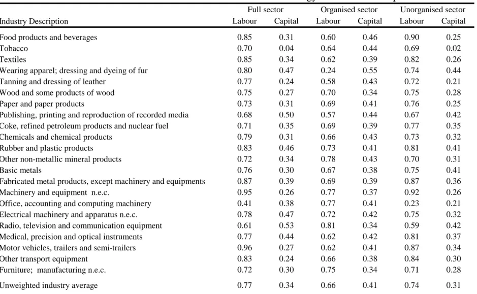
Turning to productivity estimates, table 2 reports the estimated coefficients for 22 two-digit manufacturing industries. We start with the combined estimations for the organized and unorganized sectors and then treat each sector separately. A number of important features emerge from this table.
First, the organized and unorganized sectors differ in their capital and employment intensity. The mean share of capital (i.e., total fixed assets) across industries is 0.41 in the organized sector versus 0.31 in the unorganized sector. These differences may reflect differences in access to capital or other conditions that determine the operation of establishments in both sectors. They may also capture specialization in different segments of these industries. Regardless of their origin, these differences are large enough that we want to estimate productivity allowing for factor coefficients to differ across sectors for the same industry.
20
A large majority of industries appear in Table 2 to operate under increasing returns, since the sum of the employment and capital coefficients often exceeds one. This is not an artefact of our estimation technique. Similar results are obtained when productivity is estimated with OLS techniques and modeling these two factors of production or separating the main components of capital: land, buildings, and other fixed assets. Measuring increasing returns in the ability of establishments to generate revenue is puzzling as we expect most establishments to face only imperfectly elastic demand. We believe two phenomena are at work. First, they could partly reflect true increasing returns faced by all establishments that are constrained by frictions and cannot reach their optimal size. Measured increasing returns could also reflect frictions that systematically affect larger and more productive establishments. For instance, strict labor regulations may affect large establishments more than small ones (e.g., Banerjee and Moll, 2010), so that large and more productive plants employ relatively fewer workers. This type of phenomena could then lead to coefficients on factors of production that are biased upwards in productivity estimations. That is, while plants operate under constant or decreasing returns in reality, it may look like they operate under increasing returns as more productive establishments use relatively fewer factors. Regressions could attribute differences across establishments to differences in factor usage, making factors look more productive than they really are.
We thus face the empirical challenge that we need to know establishment productivity in order to measure frictions in factor allocation across establishments. At the same time, these same frictions can distort measures of establishment productivity. To address with this problem, we duplicate our results using productivity estimates that impose constant returns to scale.
More generally, our main need here is to obtain the best possible estimate for productivity at the establishment level. For this, we focus on the LP-Sivadasan approach. We also experiment satisfactorily with OLS approaches to ensure robustness and to model more flexible functional forms that can consider more factors of production (e.g., break down total fixed assets into land, buildings, and other fixed assets). When we estimate OLS TFP with three factors of production (land and buildings, capital, and employment), the average coefficient on land and building is 0.13 and the average coefficient on other fixed assets is 0.28 in the organized sector. These two
21
coefficients sum to 0.41 which is the same as the average coefficient on TFP with our main LP estimation. When we distinguish between land and buildings, the average coefficients are 0.04 on land, 0.11 on buildings, and 0.27 on other fixed assets. These coefficients sum to just above 0.41. These elasticities of establishment value added with respect to land and buildings are used below to assess the effects of increased factor availability.
Figures 2a and 2b represent our TFP estimates averaged by district for the organized sector and unorganized sector, respectively. Like the earlier maps of output per worker, these two maps reveal a strong contrast between the more productive western parts of the country and the less productive eastern areas. These two maps also again show areas of higher productivity around India’s largest metropolitan areas, most notably Kolkata, Chennai, Bangalore and Delhi.
Although a full development or growth accounting exercise is beyond the scope of our study, a comparison of these figures is suggestive that India’s spatial disparities in output per worker are to some extent productivity disparities. There is no correlation between the organized and unorganized sectors with respect to district-level TFP.
3.5 Some descriptive facts about misallocation in India
Figures 3a and 3b provide maps of our preferred misallocation index for land and buildings in the organized and unorganized sector, respectively. Darker colors indicate greater misallocation.
Both sectors display a negative correlation between output per worker and misallocation. The more misallocated districts in the northeast, south, and interior are all districts with low output per worker. The next section documents and quantifies these relationships more precisely.
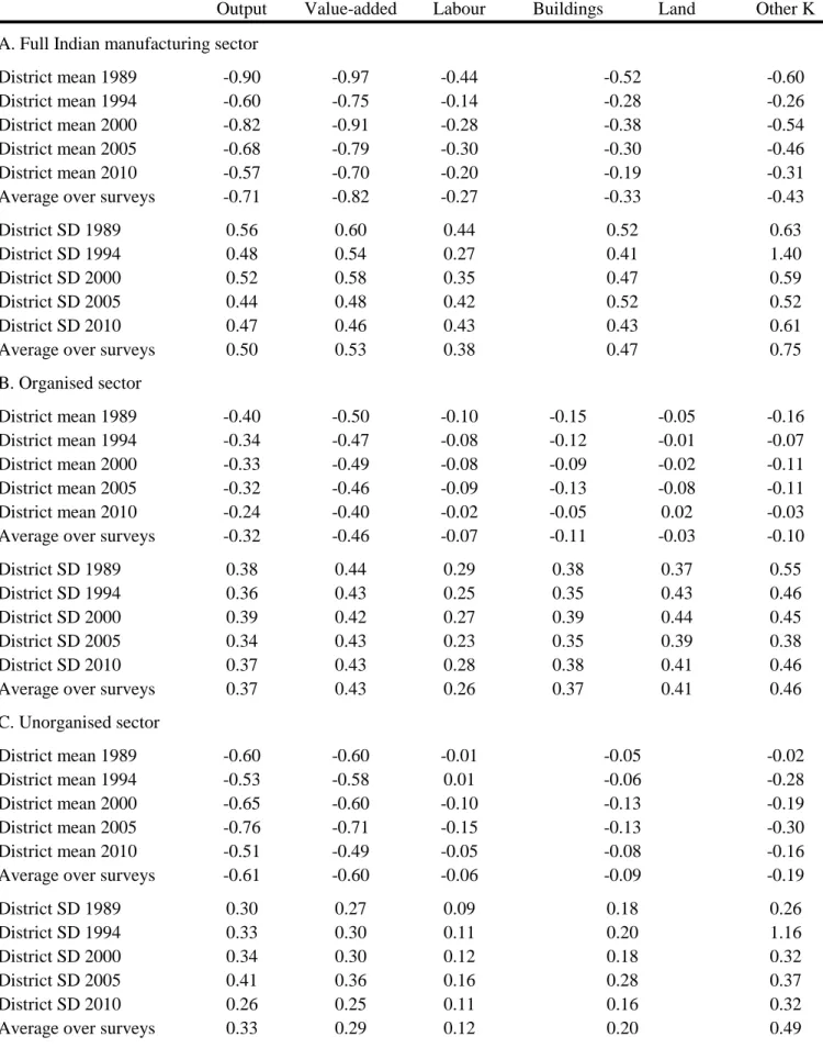
Table 3 reports descriptive statistics for indices of misallocation for Indian districts. We report statistics for the full manufacturing sector, followed by breakouts of the organized and unorganized sectors. A number of features are worth highlighting. Recalling that higher index values indicate greater misallocation, we estimate less value-added misallocation in panel A when considering the full manufacturing sector than when considering each sector independently. This is not surprising given the high concentration of output in the organized
22
sector and its more productive establishments. Combining the organized and unorganized distributions increases the correlation of these output shares and productivity.
These district-level indices for misallocation of output and value added are reasonable compared to prior literature. Bartelsman et al. (2009) compute overall input misallocation indices for 18 countries at different levels of economic development. For the sake of comparison we compute an average input factor misallocation index for the full manufacturing sector, weighting indices of factor input misallocation by their average share in production. Despite some computational differences with Bartelsman et al. (2009), these indices are roughly comparable. The mean over 1989-2010for Indian districts is about -0.33. This is marginally worse than the United States (as a whole) calculated by Bartelsman et al. (2009). More generally, Indian districts are less misallocated than the majority of the 18 countries considered by Bartelsman et al. (2009).
The second key feature of table 3 is the considerable variation of misallocation across districts.
The standard deviations for the indices of misallocation for output and value added are two- thirds of their levels for the full manufacturing sector in panel A. For the organized sector, the mean and standard deviation are comparable. This suggests considerable differences in misallocation within India, a fact not previously documented by the literature. The differences in misallocation within India are even larger than the differences across countries estimated by Bartelsman et al. (2009). The difference between the country with the lowest misallocation and that with the highest in their data is about 0.7. This corresponds to about 1.3 standard deviations for misallocation of value added in the full manufacturing sector of India, and 1.6 standard deviations in the organized sector.
A third key feature in table 3 is the extreme misallocation of individual factors of production, which contrasts with the lower levels of misallocation of output and value added. While the average 1989-2010 misallocation of output is -0.71 for the organized sector, it is only -0.27 for employment and -0.33 for buildings and land. The levels are even lower for each sector individually at approximately -0.1 for land and building factors.
23
Recall that zero values correspond to a situation where factor allocation is orthogonal to productivity. Hence, while more productive establishments manage to produce more than less productive establishments, allocations of some factors of production are barely better than random. Given the large variation in factor misallocation across districts, this actually indicates that there are many districts in India where factor allocation is worse than random. This troubling feature is vividly illustrated by figures 3a and 3b, where land and building misallocation indices are positive in about 40% of the districts.
Three candidate explanations exist for this gap between the indices of misallocation for output and value added and similar indices for individual factors of production. The first is that the data measure output much better than factors. While it is perhaps relatively easy for an establishment to know what its revenue is, it may be much harder to know what its capital is. This argument, however, could work in the opposite direction as it is not immediately obvious whether it is output or labor that is better measured. There is also an incentive for firms to hide output more than factors of production.
The second explanation is that even if factors are allocated equally across establishments (or at random), we still expect more productive establishments to produce more output. As argued above, vast differences in establishment productivity (e.g., due to managerial skill) may then explain why a reasonably low level of misallocation of output can co-exist with extreme factor misallocation. The important counterpart to this statement is that improvements in factor allocation may yield large output gains. We return to this issue below. Finally, we also need to keep in mind that a highly productive establishment with little land may be able to offset this by being particularly intensive in employment or in other forms of capital. For now, we only consider the covariance between factors and productivity but not how factors co-vary.
Finally, two more subtle patterns also emerge from table 3. First, the misallocation of employment and land is worse than the misallocation of buildings (when it can be separated from land) and other fixed assets. Second, there appears to be a mild trend towards a worsening output and factor misallocation over time.
24
As we turn to our regression analyses, our focus will be on the total misallocation in the manufacturing sector. At times, we will describe results that consider variation just within the organized or unorganized sectors. Similar to Table 3, it is important to highlight that the results for the combined sample will not be an average of these sector-level results. This is because the full sample also accounts for the fact that the frictions at the root of factor misallocation will affect whether an establishment belongs to the organized or the unorganized sector. It further captures the size of productivity differences between the sectors and their relationship to establishment scale.4
4. Validation of misallocation metrics
While a number of studies calculate and compare metrics of misallocation, there has been limited scope to validate them. An advantage of our focus on factor misallocation—and in particular land misallocation—is that we can demonstrate their general validity/usefulness by studying changes in district-level misallocation around two important policy reforms in India: the repeal of the Urban Land (Ceiling and Regulation) Act and changes in state-level stamp duties (taxes on land sales). This section shows that reforms that reduced frictions in the functioning of land markets are associated with a reduction in the misallocation of land (and also output).
Our empirical strategies are differences-in-differences estimations around policy changes. While our emphasis is mostly on the validation of our metrics, the empirical connection of land misallocation to policy determinants is interesting in its own right and worthy of close study. The ULCRA reform has the advantage of being unanticipated, and in our analyses we control for trends in many other local traits that could be correlated with policy adoption. We are cautious to note that other factors or policies might be adjusting alongside those that we study, and these unobserved factors could impact our results in terms of the likely impact of a policy reform. For
4 The following extreme example helps form intuition. Consider a situation where more productive establishments are either unaffected by frictions or completely crippled by them (i.e., frictions prevent them from hiring more than 10 workers). Whether a more productive establishment is affected is random. In this extreme case, there is no misallocation in the upper part of the employment distribution (i.e., in the organised sector) since only productive establishments unaffected by frictions are represented. On the other hand, establishments with low employment (i.e., in the unorganised sector) will either be constrained productive establishments and unconstrained poorly productive establishments. Measured misallocation will be extremely low in the organised sector and high in the unorganised sector. Combining the two sectors together will also yield a misallocation worse than any sector individually.
25
our core focus, observing these strong linkages of our misallocation indices to frictions thought to reduce allocative efficiency provides greater confidence in our measurement design and their useful for quantifying the role of factor misallocation.
4.1. The repeal of Urban Land (Ceiling and Regulation) Act
In 1976, the parliament of India enacted the Urban Land (Ceiling and Regulation) Act (ULCRA) with the main objective of limiting the concentration of urban land. ULCRA imposed ceiling limits for holdings of vacant land, prohibited transfers of land and buildings, and restricted building construction in 64 of the largest urban agglomerations (central cities and their suburbs).
More specifically, this regulation distinguished between four groups of cities. It applied to all of the largest cities and other cities with population larger than 200,000 in 1971 in 17 states and three UTs. Because the regulation applied to both ownership and ‘possession’ of land, it constrained both owners and renters (lessees). ULCRA further imposed potentially draconian penalties to offenders, including the destruction of newly built properties or the forced purchase of properties by the government at a symbolic price. Kimura (2013) describes how these regulations severely constrained the operations of the land and property markets in areas where ULCRA applied.
Despite the intentions of parliament, there is little empirical evidence that the equity objectives of ULCRA were fulfilled (Sridhar, 2010). In fact, the law artificially restricted the supply of urban land (e.g., by freezing large areas of land in legal dispute), bid up land prices, and encouraged corruption (Joshi and Little, 1991; Bertaud, 2002). Importantly, ULCRA also prevented private developers from assembling land for subsequent development. For almost a quarter century, ULCRA practically halted legal development of land by the private sector in urban areas unless exemptions were obtained (Srinivas, 1991). The regulation and market constraints reduced the incentives of landholders to invest in building construction. Thus, a large proportion of firms were both land and building constrained by way of ULCRA.
In 1999, the Repeal Act gave rights to state governments of India to repeal ULCRA. The ULCRA reform was mostly anticipated. A number of states and UTs repealed ULCRA by 2003,
26
including Delhi, Gujarat, Haryana, Karnataka, Madhya Pradesh, Orissa, Punjab, Rajasthan, and Uttar Pradesh. By contrast, Andhra Pradesh, Assam, Bihar, Maharashtra, and West Bengal kept ULCRA effective until 2008.5
To assess the effects of the repeal of ULCRA on misallocation, we estimate a series of regressions where we consider the district-level change in misallocation from 2000 to 2010 as the dependent variable. Our key explanatory variable is an indicator variable for states that repealed ULCRA early, as listed above. We consider the set of late adopters to be the control group as repeals in 2008 are unlikely to have substantial consequences by 2010, especially for ASI establishments surveyed in 2009-10. Estimations are unweighted cross-sectional regressions that include 252 Indian districts. We cluster standard errors by state to represent the state-level choices being made to repeal ULCRA.
𝑀𝑖,2010𝐿 − 𝑀𝑖,2000𝐿 = 𝑎0+ 𝑎1𝐸𝑎𝑟𝑙𝑦𝑅𝑒𝑝𝑒𝑎𝑙𝑖𝑈𝐿𝐶𝑅𝐴+ 𝑏1𝑋𝑖+ 𝜖𝑖
Two main estimation worries are that the repeal of ULCRA may have coincided with other district features that affected misallocation and that the initial sample of ULCRA districts may have been highly selected in a way that affects the results. To minimize these worries, we include a number of control variables X. The most essential is the initial level of misallocation. This is important because districts where ULCRA applied may have experienced greater misallocation in 2000. We also have a battery of additional controls for the initial traits of districts (e.g., population density, local demographics, local infrastructure traits) as listed in the notes to table 4.
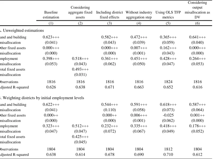
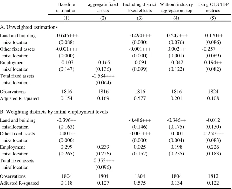
Table 4 reports our main results for the effect of the repeal of ULCRA. Panel A considers misallocation of land and buildings as the outcome variable. We focus on estimations that consider the full manufacturing sector, combining the organized and unorganized sectors together. The negative coefficient indicates that the early state-level repeal of ULCRA is associated with a stronger decline in land and building misallocation during 2000 to 2010
5 The negative effect of ULCRA is still evident in the land use patterns of Mumbai, many years after ULCRA was abrogated by the State of Maharashtra in 2007 (Bertaud, 2011). Siddiqi (2013) provides an in-depth analysis of the political economy of ULCRA adoption and its repeal in Mumbai (Maharashtra). With the repeal of ULCRA in 1999, about 25,000 acres of land have been freed. However, only 10,000 of these are in developable zones, while the remaining 15,000 fall in areas with restrictions—such as coastal zones and forest lands (Sridhar, 2010).
27
compared to late adopters. The 0.057 coefficient is quite substantial and represents about one- tenth of a standard deviation of land and building misallocation. Using results later reported in Table 7, the 0.057 decrease in misallocation for land and buildings of associated with the repeal of ULCRA corresponds to an increase in output per worker of about 3.7%.
Panel b considers the change in misallocation for value added for districts. ULCRA is associated with reduced misallocation on this dimension as well. In fact, it appears the declines may have been greater here than on land and buildings in economic terms. In terms of standard deviations, the ULCRA repeal is associated with a decline of about one-fifth of a standard deviation in value added. This larger impact may seem puzzling to start, but it is quite possible under the scenarios highlighted above where improved factor allocation is magnified by inherent differences in establishment productivity (e.g., better land access is amplified by a capable manager). Current research is also considering whether the improved functioning of land and property markets aids in other factor acquisition through improved property rights and borrowing conditions. As suggestive evidence, unreported analyses find the allocation of other fixed assets also improved with ULCRA’s repeal.
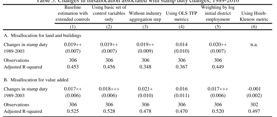
Column 2 shows this result is robust to adjustments in the covariates modeled, although the basic controls are important for the statistical precision with which we can measure ULCRA’s effect due to many other changes underway in India during this period. Columns 3-6 show that these results are quite robust to variations in methodology. We show similar findings when misallocation is computed without aggregating first by industry, when using OLS estimates of productivity, when weighting districts by initial employment, and when following the HK approach. The results are actually stronger statistically than our primary metrics in column 1.
The point estimates of the coefficients are not directly comparable due to the different scales and variances of the metrics. The results are also robust to different approaches towards extreme values like winsorization.
Unreported estimations consider misallocation in distributions specific to the organized and unorganized sectors. The repeal of ULCRA is more closely associated with reduced misallocation for factors in the unorganized sector than the organized sector: the unorganized
28
sector coefficient is -0.035 (se=0.021), which represents again a tenth of a standard deviation for the sector. Yet, it is quite clear overall that the major impact of ULCRA came less from changes in misallocation within each sector vs. changes in the relative sizes of sectors and their joint distribution for misallocation. As one example, the log change in the value of land and buildings in the organized sector with ULCRA’s repeal is 0.722 (se=0.261) for the organized sector, compared to 0.420 (se=0.197) for the unorganized sector. These relative changes in factor allocations across sectors appear to have been more central for the reductions in misallocation compared to changes within sectors.
4.2 Stamp duty
High stamp duties are another trait of Indian property markets.6 These taxes are collected whenever a real property is transacted. While these taxes are between zero and 5% in most North American jurisdictions, they tend to be much higher in India. There is also a lot of variation across states and time. For instance, the lowest rate is found in Tripura at 5%, while the highest rate of 21.2% was in West Bengal early in our period of study. West Bengal dramatically lowered its stamp duty, reaching 5% in 2003. These taxes represent an important friction and have received some academic attention outside of India, affecting for example the Canadian housing market by lowering prices and the number of transactions (e.g., Dachis et al., 2012).
High stamp duties impose high compliance costs on taxpayers and lead to widespread avoidance through under-reporting (Alm et al, 2004; Morris and Pandey, 2009). This in turn adversely affects the possibility of using land as collateral for construction financing. High stamp duties also discourage land transactions, and as a consequence reduce the supply of land on the market.
High stamp duties are thought to be at the root of a $3.4 billion scam on the use of fraudulent stamp papers by Abdul Karim Telgi that was reported in India in 2002.
6 Stamp duties in India are imposed under the Indian Stamp Act, 1899, as amended several times over the years at the central government level. Under these central acts, each state has the authority to enact its own stamp duties, so that the specific features of the stamp duties, while broadly similar across the states, also take on state-specific characteristics. Within the broad definition of stamp duties imposed on sale and purchase of business transactions, including property, there are two sub-classifications: (i) Judicial stamp duty is usually a small fee collected by the court for litigation purposes, and (ii) Non-judicial stamp duty is a onetime charge on the transfer of immovable property based on the value of the transaction.