Dynamic Mechanisms without Money

IHS Economics Series Working Paper 310

March 2015

Dynamic Mechanisms without Money

Yingni Guo

Johannes Hörner

Impressum Author(s):

Yingni Guo, Johannes Hörner Title:

Dynamic Mechanisms without Money ISSN: Unspecified

2015 Institut für Höhere Studien - Institute for Advanced Studies (IHS) Josefstädter Straße 39, A-1080 Wien

E-Mail: o ce@ihs.ac.at ffi Web: ww w .ihs.ac. a t

All IHS Working Papers are available online: http://irihs. ihs. ac.at/view/ihs_series/

This paper is available for download without charge at:

https://irihs.ihs.ac.at/id/eprint/3129/

Dynamic Mechanisms without Money

Yingni Guo

and Johannes Hörner

1

Northwestern University

2

Yale University

March 2015

All IHS Working Papers in Economics are available online:

https://www.ihs.ac.at/library/publications/ihs-series/

Economics Series

Working Paper No. 310

Dynamic Mechanisms without Money ^∗

Yingni Guo ^† , Johannes Hörner ^‡ March 2015

Abstract

We analyze the optimal design of dynamic mechanisms in the absence of transfers.

The designer uses future allocation decisions to elicit private information. Values evolve according to a two-state Markov chain. We solve for the optimal allocation rule, which permits a simple implementation. Unlike with transfers, efficiency decreases over time, and both immiseration and its polar opposite are possible long-run outcomes. Con- sidering the limiting environment in which time is continuous, we demonstrate that persistence hurts.

Keywords: Mechanism design. Principal-Agent. Token mechanisms.

JEL numbers: C73, D82.

1 Introduction

This paper is concerned with the dynamic allocation of resources when transfers are not allowed and information regarding their optimal use is private information to an individual.

The informed agent is strategic rather than truthful.

We are searching for the social choice mechanism that would bring us closest to efficiency.

Here, efficiency and implementability are understood to be Bayesian: both the individual and society understand the probabilistic nature of uncertainty and update based on it.

∗

We thank Alex Frankel, Drew Fudenberg, Juuso Toikka and Alex Wolitzky for very useful conversations.

†

Department of Economics, Northwestern University, 2001 Sheridan Rd., Evanston, IL 60201, USA, yingni.guo@northwestern.edu.

‡

Yale University, 30 Hillhouse Ave., New Haven, CT 06520, USA, johannes.horner@yale.edu.

Both the societal decision not to allow money –for economic, physical, legal or ethical reasons– and the sequential nature of the problem are assumed. Temporal constraints apply to the allocation of goods, such as jobs, houses or attention, and it is often difficult to ascertain future demands.

Throughout, we assume that the good to be allocated is perishable.

Absent private information, the allocation problem is trivial: the good should be provided if and only if its value exceeds its cost.

However, in the presence of private information, and in the absence of transfers, linking future allocation decisions to current decisions is the only instrument available to society to elicit truthful information. Our goal is to understand this link.

Our main results are a characterization of the optimal mechanism and an intuitive in- direct implementation for it. In essence, the agent should be granted an inside option, corresponding to a certain number of units of the good that he is entitled to receive “no questions asked.” This inside option is updated according to his choice: whenever the agent desires the unit, his inside option is reduced by one unit; whenever he forgoes it, his inside option is also revised, although not necessarily upward. Furthermore, we demonstrate that this results in very simple dynamics: an initial phase of random length in which the efficient choice is made during each round, followed by an irreversible shift to one of the two possible outcomes in the game with no communication, namely, the unit is either always supplied or never supplied again. These results contrast with those from static design with multiple units (e.g., Jackson and Sonnenschein, 2007) and from dynamic mechanism design with transfers (e.g., Battaglini, 2005).

Formally, our good can take one of two values during each round. Values are serially correlated over time. The binary assumption is certainly restrictive, but it is known that, even with transfers, the problem becomes intractable beyond binary types (see Battaglini and Lamba, 2014).

We begin with the i.i.d. case, which suffices to illustrate many of the insights of our analysis, before proving the results in full generality. The cost of providing the good is fixed and known. Hence, it is optimal to assign the good during a given round if and only if the value is high. We cast our problem of solving for the efficient mechanism (given the values, cost and agent’s discount factor) as one faced by a disinterested principal with

1

Many allocation decisions involve goods or services that are perishable, such as how a nurse or a worker should divide time; which patients should receive scarce medical resources (blood or treatments); or which investments and activities should be approved by a firm.

2

This is because the supply of the perishable good is taken as given. There is a considerable literature on the optimal ordering policy for perishable goods, beginning with Fries (1975).

3

In Section 5.2, we consider the case of a continuum of types that are independently distributed over

time.

commitment who determines when to supply the good as a function of the agent’s reports.

There are no transfers, certification technology, or signals concerning the agent’s value, even ex post.

As mentioned above, we demonstrate that the optimal policy can be implemented through a “budget” mechanism in which the appropriate unit of account is the number of units that the agent is entitled to receive sequentially with “no questions asked.” While the updating process when the agent forgoes a unit is somewhat subtle, it is independent of the principal’s belief concerning the agent’s type. The only role of the prior belief is to specify the initial budget. This budget mechanism is not a token mechanism in the sense that the total (discounted) number of units the agent receives is not fixed. Depending on the sequence of reports, the agent might ultimately receive few or many units.

Eventually, the agent is either granted the unit forever or never again. Hence, immiseration is not ineluctable.

In Section 5.1, we study the continuous time limit over which the flow value for the good changes according to a two-state Markov chain. This allows us to demonstrate that persis- tence hurts. As the Markov chain becomes more persistent, efficiency decreases, although the agent might actually benefit from this increased persistence.

Allocation problems in the absence of transfers are plentiful, and it is not our purpose to survey them here. We believe that our results can inform practices concerning how to implement algorithms to improve allocations. For example, consider nurses who must decide whether to take alerts that are triggered by the patients seriously. The opportunity cost of their time is significant. Patients, however, appreciate quality time with nurses irrespective of whether their condition necessitates it. This discrepancy produces a challenge with which every hospital must contend: ignore alarms and risk that a patient with a serious condition is not attended to or heed all alarms and overwhelm the nurses. “Alarm fatigue” is a serious problem that health care must confront (see, for instance, Sendelbach, 2012). We suggest the best approach for trading off the risks of neglecting a patient in need and attending to one who simply cries wolf.

Related Literature. Our work is closely related to the bodies of literature on mechanism design with transfers and on “linking incentive constraints.” Sections 4.5 and 3.4 are devoted to these issues and explain why transfers (resp., the dynamic nature of the relationship)

4

It is not a “bankruptcy” mechanism in the sense of Radner (1986) because the specific ordering of the reports matters.

5

Clearly, our mechanism is much simpler than existing electronic nursing workload systems. However,

none appears to seriously consider strategic agent behavior as a constraint.

matter, and hence, we will brief here.

The obvious benchmark work that considers transfers is Battaglini (2005),

who considers our general model but allows transfers. Another important difference is his focus on revenue maximization, a meaningless objective in the absence of prices. The results of his work are diametrically opposed to ours. In Battaglini, efficiency necessarily improves over time (exact efficiency is eventually obtained with probability 1). Here, efficiency decreases over time, in the sense described above, with an asymptotic outcome that is at best the outcome of the static game. The agent’s utility can increase or decrease depending on the history that is realized: receiving the good forever is clearly the best possible outcome, while never receiving it again is the worst outcome. Krishna, Lopomo and Taylor (2013) provide an analysis of limited liability (though transfers are allowed) in a model closely related to that of Battaglini, suggesting that excluding the possibility of unlimited transfers affects both the optimal contract and dynamics. Note that there is an important exception to the quasi- linearity commonly assumed in the dynamic mechanism design literature, namely, Garrett and Pavan (2015).

“Linking incentive constraints” refers to the notion that as the number of identical decision problems increases, linking them allows the designer to improve on the isolated problem.

See Fang and Norman (2006) and Jackson and Sonnenschein (2007) for papers specifically devoted to this idea (although they are much older, see Radner, 1981; Rubinstein and Yaari, 1983). Hortala-Vallve (2010) provides an interesting analysis of the unavoidable inefficiencies that must be incurred away from the limit, and Cohn (2010) demonstrates the suboptimality of the mechanisms that are commonly used, even regarding the rate of convergence. Our focus is on the exactly optimal mechanism for a fixed degree of patience, not on proving the asymptotic optimality of a specific mechanism (numerous mechanisms yield asymptotic optimality). This focus allows us to estimate the rate of convergence. Another important difference from most of these papers is that our problem is truly dynamic in the sense that the agent does not know future values but learns them as they come. Section 3.4 elaborates on this distinction.

The notion that virtual budgets could be used as intertemporal instruments to discipline agents with private information has appeared in several papers in economics. Möbius (2001) might be the first to suggest that tracking the difference in the number of favors granted (with two agents) and using it to decide whether to grant new favors is a simple but powerful way of sustaining cooperation in long-run relationships. See also Athey and Bagwell (2001),

6

See also Zhang (2012) for an exhaustive analysis of Battaglini’s model as well as Fu and Krishna (2014).

Abdulkadiroğlu and Bagwell (2012) and Kalla (2010). While these token mechanisms are known to be suboptimal (as is clear from our characterization of the optimal mechanism), they have desirable properties nonetheless: properly calibrated, they yield an approximately efficient allocation as the discount factor approaches one. To our knowledge, Hauser and Hopenhayn (2008) come the closest to solving for the optimal mechanism (within the class of PPE). Their numerical analysis allows them to qualify the optimality of simple budget rules (according to which each favor is weighted equally, independent of the history), showing that this rule might be too simple (the efficiency cost can reach 30% of surplus). Remarkably, their analysis suggests that the optimal (Pareto-efficient) strategy shares many common fea- tures with the optimal policy that we derive in our one-player world: the incentive constraint always binds, and the efficient policy is followed unless it is inconsistent with promise keeping (meaning when promised utilities are too extreme). Our model can be regarded as a game with one-sided incomplete information in which the production cost of the principal is known to the second player. There are some differences, however. First, our principal has commit- ment and hence is not tempted to act opportunistically or bound by individual rationality.

Second, this principal maximizes efficiency rather than his own payoff. Third, there is a technical difference: our limiting model in continuous time corresponds to the Markovian case in which flow values switch according to a Poisson process. In Hauser and Hopenhayn, the lump-sum value arrives according to a Poisson process, and the process is memoryless.

Li, Matouschek and Powell (2015) solve for the perfect public equilibria in a model similar to our i.i.d. benchmark and allow for monitoring (public signals), demonstrating that better monitoring improves performance.

More generally, that allocation rights to other (or future) units can be used as a “currency”

to elicit private information has long been recognized and dates to Hylland and Zeckhauser (1979), who first explained the extent to which this can be viewed as a pseudo-market.

Casella (2005) develops a similar idea within the context of voting rights. Miralles (2012) solves a two-unit version of our problem with more general value distributions, but his analysis is not dynamic: both values are (privately) known at the outset. A dynamic two- period version of Miralles is analyzed by Abdulkadiroğlu and Loertscher (2007).

All versions considered in this paper would be trivial in the absence of imperfect obser-

vation of the values. If the values were perfectly observed, it would be optimal to assign the

good if and only if the value is high. Due to private information, it is necessary to distort

the allocation: after some histories, the good is provided independent of the report; after

others, the good is never provided again. In this sense, the scarcity of goods provision is

endogenously determined to elicit information. There is a large body of literature in opera-

tions research considering the case in which this scarcity is considered exogenous – there are only n opportunities to provide the good, and the problem is then when to exercise these opportunities. Important early contributions to this literature include Derman, Lieberman and Ross (1972) and Albright (1977). Their analyses suggest a natural mechanism that can be applied in our environment: the agent receives a certain number of “tokens” and uses them whenever he pleases.

Exactly optimal mechanisms have been computed in related environments. Frankel (2011) considers a variety of related settings. The most similar is his Chapter 2 analysis in which he also derives an optimal mechanism. While he allows for more than two types and actions, he restricts attention to the types that are serially independent over time (our starting point). More importantly, he assumes that the preferences of the agent are inde- pendent of the state, which allows for a drastic simplification of the problem. Gershkov and Moldovanu (2010) consider a dynamic allocation problem related to Derman, Lieberman and Ross in which agents possess private information regarding the value of obtaining the good.

In their model, agents are myopic and the scarcity of the resource is exogenously assumed.

In addition, transfers are allowed. They demonstrate that the optimal policy of Derman, Lieberman and Ross (which is very different from ours) can be implemented via appropriate transfers. Johnson (2013) considers a model that is more general than ours (he permits two agents and more than two types). Unfortunately, he does not provide a solution to his model.

A related literature considers the related problem of optimal stopping in the absence of transfers; see, in particular, Kováč, Krähmer and Tatur (2014). This difference reflects the nature of the good, namely, whether it is perishable or durable. When only one unit is desired and waiting is possible, this represents a stopping problem, as in their paper. With a perishable good, a decision must be made during every round. As a result, incentives (and the optimal contract) have hardly anything in common. In the stopping case, the agent might have an option value to forgo the current unit if the value is low and future prospects are good. This is not the case here – incentives to forgo the unit must be endogenously generated via promises. In the stopping case, there is only one history of outcomes that does not terminate the game. Here, policies differ not only in when the good is first provided but also thereafter.

Finally, while the motivations of the papers differ, the techniques for the i.i.d. benchmark that we use borrow numerous ideas from Thomas and Worrall (1990), as we explain in Section 3, and our intellectual debt is considerable.

Section 2 introduces the model. Section 3 solves the i.i.d. benchmark, introducing most

of the ideas of the paper, while Section 4 solves the general model. Section 5 extends the

results to cases of continuous time or continuous types. Section 6 concludes.

2 The Model

Time is discrete and the horizon infinite, indexed by n = 0, 1, . . .. There are two parties, a disinterested principal and an agent. During each round, the principal can produce an indivisible unit of a good at a cost c > 0. The agent’s value (or type ) during round n, v

is a random variable that takes value l or h. We assume that 0 < l < c < h such that supplying the good is efficient if and only if the value is high, but the agent’s value is always positive.

The value follows a Markov chain as follows:

P [v

= h | v

= h] = 1 − ρ

, P [v

= l | v

= l] = 1 − ρ

,

for all n ≥ 0, where ρ

, ρ

∈ [0, 1]. The (invariant) probability of h is q := ρ

/(ρ

+ ρ

).

For simplicity, we also assume that the initial value is drawn according to the invariant distribution, that is, P [v

= h] = q. The (unconditional) expected value of the good is denoted µ := E [v] = qh + (1 − q)l. We make no assumptions regarding how µ compares to c.

Let κ := 1 − ρ

− ρ

be a measure of the persistence of the Markov chain. Throughout, we assume that κ ≥ 0 or, equivalently, 1 − ρ

≥ ρ

; that is, the distribution over tomorrow’s type conditional on today’s type being h first-order stochastically dominates the distribution conditional on today’s type being l.

Two interesting special cases occur when κ = 1 and κ = 0. The former corresponds to perfect persistence, while the latter corresponds to independent values.

The agent’s value is private information. Specifically, at the beginning of each round, the value is drawn and the agent is informed of it.

Players are impatient and share a common discount factor δ ∈ [0, 1).

To exclude trivi- alities, we assume throughout that δ > l/µ and δ > 1/2.

Let x

∈ { 0, 1 } refer to the supply decision during round n; e.g., x

= 1 means that the good is supplied during round n.

7

The role of this assumption, which is commonly adopted in the literature, and what occurs in its absence, when values are negatively serially correlated, is discussed at the end of Sections 4.3 and 4.4.

8

The common discount factor is important. We view our principal as a social planner trading off the

agent’s utility with the social cost of providing the good as opposed to an actual player. As a social planner

internalizing the agent’s utility, it is difficult to understand why his discount rate would differ from the

agent’s.

Our focus is on identifying the (constrained) efficient mechanism defined below. Hence, we assume that the principal internalizes both the cost of supplying the good and the value of providing it to the agent. We solve for the principal’s favorite mechanism.

Thus, given an infinite history { x

, v

}

, the principal’s realized payoff is defined as follows:

(1 − δ) X

n=0

δ

x

(v

− c),

where δ ∈ [0, 1) is a discount factor. The agent’s realized utility is defined as follows:

(1 − δ)

∞

X

n=0

δ

x

v

.

Throughout, payoff and utility refer to the expectation of these values given the relevant player’s information. Note that the utility belongs to the interval [0, µ].

The (risk-neutral) agent seeks to maximize his utility. We now introduce or emphasize several important assumptions maintained throughout our analysis.

- There are no transfers. This is our point of departure from Battaglini (2005) and most of the previous research on dynamic mechanism design. Note also that our objective is efficiency, not revenue maximization. With transfers, there is a trivial mechanism that achieves efficiency: supply the good if and only if the agent pays a fixed price in the range (l, h).

- There is no ex post signal regarding the realized value of the agent –not even payoffs are observed. Depending on the context, it might be realistic to assume that a (possibly noisy) signal of the value occurs at the end of each round, independent of the supply decision. In some other economic examples, it might make more sense to assume instead that this signal occurs only if the good is supplied (e.g., a firm discovers the productivity of a worker who is hired). Conversely, statistical evidence might only occur from not supplying the good if supplying it averts a risk (a patient calling for care or police calling for backup). See Li, Matouschek and Powell (2014) for such an analysis (with “public shocks”) in a related context. Presumably, the optimal mechanism will differ according to the monitoring structure. Understanding what happens without any signal is the natural first step.

- We assume that the principal commits ex ante to a (possibly randomized) mechanism.

This assumption brings our analysis closer to the literature on dynamic mechanism

9

Throughout, the term payoff describes the principal’s objective and utility describes the agent’s.

design and distinguishes it from the literature on chip mechanisms (as well as Li, Matouschek and Powell, 2014), which assumes no commitment on either side and solves for the (perfect public) equilibria of the game.

- The good is perishable. Hence, previous choices affect neither feasible nor desirable future opportunities. If the good were perfectly durable and only one unit were de- manded, the problem would be one of stopping, as in Kováč, Krähmer and Tatur (2014).

Due to commitment by the principal, we focus on policies in which the agent truthfully reports his type during every round and the principal commits to a (possibly random) supply decision as a function of this last report as well as of the entire history of reports without a loss of generality.

Formally, a direct mechanism or policy is a collection ( x

)

, with x

: { l, h }

→ [0, 1]

(with { l, h }

:= {∅} ),

mapping a sequence of reports by the agent into a decision to supply the good during a given round. Our definition exploits the fact that, because preferences are time-separable, the policy may be considered independent of past realized supply decisions.

A direct mechanism defines a decision problem for the agent who seeks to maximize his utility. A reporting strategy is a collection ( m

)

, where m

: { l, h }

× { l, h } → ∆( { l, h } ) maps previous reports and the value during round n into a report for that round.

The policy is incentive compatible if truth-telling (that is, reporting the current value faithfully, independent of past reports) is an optimal reporting strategy.

Our first objective is to solve for the optimal (incentive-compatible) policy, that is, for the policy that maximizes the principal’s payoff subject to incentive compatibility. The value is the resulting payoff. Second, we would like to find a simple indirect implementation of this policy. Finally, we wish to understand the payoff and utility dynamics under this policy.

3 The i.i.d. Benchmark

We begin our investigation with the simplest case in which values are i.i.d. over time; that is, κ = 0. This is a simple extension of Thomas and Worrall (1990), although the indivisibility caused by the absence of transfers leads to dynamics that differ markedly from theirs. See Section 4 for the analysis in the general case κ ≥ 0.

10

For simplicity, we use the same symbols l, h for the possible agent reports as for the values of the good.

11

Without a loss of generality, we assume that this strategy does not depend on past values, given past

reports, as the decision problem from round n onward does not depend on these past values.

With independent values, it is well known that attention can be further restricted to policies that can be represented by a tuple of functions U

, U

: [0, µ] → [0, µ], p

, p

: [0, µ] → [0, 1] mapping a utility U (interpreted as the continuation utility of the agent) onto a continuation utility u

= U

(U), u

= U

(U) beginning during the next round as well as the probabilities p

(U), p

(U) of supplying the good during this round given the current report of the agent. These functions must be consistent in the sense that, given U , the probabilities of supplying the good and promised continuation utilities yield U as a given utility to the agent. This is “promise keeping.” We stress that U is the ex ante utility in a given round;

that is, it is computed before the agent’s value is realized. The reader is referred to Spear and Srivastava (1987) and Thomas and Worrall (1990) for details.

Because such a policy is Markovian with respect to the utility U, the principal’s payoff is also a function of U only. Hence, solving for the optimal policy and the (principal’s) value function W : [0, µ] → R amounts to a Markov decision problem. Given discounting, the optimality equation characterizes both the value and the (set of) optimal policies. For any fixed U ∈ [0, µ], the optimality equation states the following:

W (U ) = sup

ph,pl,uh,ul

{ (1 − δ) (qp

(h − c) + (1 − q)p

(l − c))

+ δ (qW (u

) + (1 − q)W (u

)) } (OBJ) subject to incentive compatibility and promise keeping, namely,

(1 − δ)p

h + δu

≥ (1 − δ)p

h + δu

, (IC

) (1 − δ)p

l + δu

≥ (1 − δ)p

l + δu

, (IC

) U = (1 − δ) (qp

h + (1 − q)p

l) + δ (qu

+ (1 − q)u

) , (P K)

(p

, p

, u

, u

) ∈ [0, 1] × [0, 1] × [0, µ] × [0, µ].

The incentive compatibility and promise keeping conditions are denoted IC (IC

, IC

) and P K. This optimization program is denoted P .

Our first objective is to calculate the value function W as well as the optimal policy.

Obviously, the entire map might not be relevant once we account for the specific choice of the initial promise –some promised utilities might simply never arise for any sequence of reports. Hence, we are also interested in solving for the initial promise U

, the maximizer of the value function W .

12

Note that not every policy can be represented in this fashion, as the principal does not need to treat two

histories leading to the same continuation utility identically. However, because they are equivalent from the

agent’s viewpoint, the principal’s payoff must be maximized by some policy that does so.

3.1 Complete Information

Consider the benchmark case in which there is complete information: that is, consider P without the IC constraints. As the values are i.i.d., we can assume, without loss of generality, that p

, p

are constant over time. Given U , the principal chooses p

and p

to maximize

qp

(h − c) + (1 − q)p

(l − c), subject to U = qp

h + (1 − q)p

l. It follows easily that

Lemma 1 Under complete information, the optimal policy is







p

=

, p

= 0 if U ∈ [0, qh], p

= 1, p

=

if U ∈ [qh, µ].

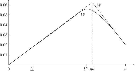
The value function, denoted W ¯ , is equal to W ¯ (U ) =







1 −

U if U ∈ [0, qh],

1 −

U + cq

− 1

if U ∈ [qh, µ].

Hence, the initial promise (maximizing W ¯ ) is U

:= qh.

That is, unless U = qh, the optimal policy (p

, p

) cannot be efficient. To deliver U < qh, the principal chooses to scale down the probability with which to supply the good when the value is high, maintaining p

= 0. Similarly, for U > qh, the principal is forced to supply the good with positive probability even when the value is low to satisfy promise keeping.

While this policy is the only constant optimal one, there are many other (non-constant) optimal policies. We will encounter some in the sequel.

We call W ¯ the complete-information payoff function. It is piecewise linear (see Figure 1). Plainly, it is an upper bound to the value function under incomplete information.

3.2 The Optimal Mechanism

We now solve for the optimal policy under incomplete information in the i.i.d. case. We first provide an informal derivation of the solution. It follows from two observations (formally established below). First,

The efficient supply choice (p

, p

) = (0, 1) is made “as long as possible.”

To understand this qualification, note that if U = 0 (resp., U = µ), promise keeping allows no latitude in the choice of probabilities. The good cannot (or must) be supplied, independent of the report. More generally, if U ∈ [0, (1 − δ)qh), it is impossible to supply the good if the value is high while satisfying promise keeping. In this utility range, the observation must be interpreted as indicating that the supply choice is as efficient as possible given the restriction imposed by promise keeping. This implies that a high report leads to a continuation utility of 0, with the probability of the good being supplied adjusting accordingly. An analogous interpretation applies to U ∈ (µ − (1 − δ)(1 − q)l, µ].

These two peripheral intervals vanish as δ → 1 and are ignored for the remainder of this discussion. For every other promised utility, we claim that it is optimal to make the (“static”) efficient supply choice. Intuitively, there is never a better time to redeem part of the promised utility than when the value is high. During such rounds, the interests of the principal and agent are aligned. Conversely, there cannot be a worse opportunity to repay the agent what he is due than when the value is low because tomorrow’s value cannot be lower than today’s.

As trivial as this observation may sound, it already implies that the dynamics of the inefficiencies must be very different from those in Battaglini’s model with transfers. Here, inefficiencies are backloaded.

As the supply decision is efficient as long as possible, the high type agent has no incentive to pretend to be a low type. However,

Incentive compatibility of the low type agent always binds.

Specifically, without a loss of generality, assume that IC

always binds and disregard IC

. The reason that the constraint binds is standard: the agent is risk neutral, and the principal’s payoff must be a concave function of U (otherwise, he could offer the agent a lottery that the agent would be willing to accept and that would make the principal better off). Concavity implies that there is no gain in spreading continuation utilities u

, u

beyond what is required for IC

to be satisfied.

Because we are left with two variables (u

, u

) and two constraints (IC

and P K), we can immediately solve for the optimal policy. Algebra is not needed. Because the agent is always willing to state that his value is high, it must be the case that his utility can be computed as if he followed this reporting strategy, namely,

U = (1 − δ)µ + δu

, or u

= U − (1 − δ)µ

δ .

Because U is a weighted average of u

and µ ≥ U , it follows that u

≤ U . The promised utility necessarily decreases after a high report. To compute u

, note that the reason that the high type agent is unwilling to pretend he has a low value is that he receives an incremental value (1 − δ)(h − l) from obtaining the good relative to what would make him merely indifferent between the two reports. Hence, defining U := q(h − l), it holds that

U = (1 − δ)U + δu

, or u

= U − (1 − δ)U

δ .

Because U is a weighted average of U and u

, it follows that u

≤ U if and only if U ≤ U. In that case, even a low report leads to a decrease in the continuation utility, albeit a smaller decrease than if the report had been high and the good provided.

The following theorem (proved in the appendix, as are all other results) summarizes this discussion with the necessary adjustments on the peripheral intervals.

Theorem 1 The unique optimal policy is p

= max

0, 1 − µ − U (1 − δ)l

, p

= min

1, U (1 − δ)µ

. Given these values of (p

, p

), continuation utilities are

u

= U − (1 − δ)p

µ

δ , u

= U − (1 − δ)(p

l + (p

− p

)U )

δ .

For reasons that will become clear shortly, this policy is not uniquely optimal for U ≤ U . We now turn to a discussion of the utility dynamics and of the shape of the value function, which are closely related. This discussion revolves around the following lemma.

Lemma 2 The value function W : [0, µ] → R is continuous and concave on [0, µ], contin- uously differentiable on (0, µ), linear (and equal to W ¯ ) on [0, U], and strictly concave on [U , µ]. Furthermore,

lim

W

(U ) = 1 − c

h , lim

U↑µ

W

(U ) = 1 − c l .

Indeed, consider the following functional equation for W that we obtain from Theorem 1 (ignoring again the peripheral intervals for the sake of the discussion):

W (U ) = (1 − δ)q(h − c) + δqW

U − (1 − δ)µ δ

+ δ(1 − q)W

U − (1 − δ)U δ

. Hence, taking for granted the differentiability of W stated in the lemma,

W

(U) = qW

(U

) + (1 − q)W

(U

).

In probabilistic terms, W

(U

) = E [W

(U

)] given the information at round n. That is, W

is a bounded martingale and must therefore converge.

This martingale was first uncovered by Thomas and Worrall (1990), and hence, we refer to it as the TW-martingale. Because W is strictly concave on (U, µ), yet u

6 = u

in this range, it follows that the process { U

}

must eventually exit this interval. Hence, U

must converge to either U

= 0 or µ. However, note that, because u

< U and u

≤ U on the interval (0, U ], this interval is a transient region for the process. Hence, if we began this process in the interval [0, U ], the limit must be 0 and the TW-martingale implies that W

must be constant on this interval – hence the linearity of W .

While W

:= W

(U

) is a martingale, U

is not. Because the optimal policy yields U

= (1 − δ)qh + δ E [U

],

utility drifts up or down (stochastically) according to whether U = U

is above or below qh. Intuitively, if U > qh, then the flow utility delivered is insufficient to honor the average promised utility. Hence, the expected continuation utility must be even larger than U .

This raises the question of the initial promise U

: does it lie above or below qh, and where does the process converge given this initial value? The answer is provided by the TW- martingale. Indeed, U

is characterized by W

(U

) = 0 (uniquely so, given strict concavity on [U , µ]). Hence,

0 = W

(U

) = P [U

= 0 | U

= U

]W

(0) + P [U

= µ | U

= U

]W

(µ), where W

(0) and W

(µ) are the one-sided derivatives given in the lemma. Hence,

P [U

= 0 | U

= U

]

P [U

= µ | U

= U

] = (c − l)/l

(h − c)/h . (1)

The initial promise is chosen to yield this ratio of absorption probabilities at 0 and µ.

Remarkably, this ratio is independent of the discount factor (despite the discrete nature of the random walk, the step size of which depends on δ!). Hence, both long-run outcomes are possible irrespective of how patient the players are. However, depending on the parameters, U

can be above or below qh, the first-best initial promise, as is easy to confirm through examples. In the appendix, we demonstrate that U

is decreasing in the cost, which should

13

It is bounded because W is concave, and hence, its derivative is bounded by its value at 0 and µ, given in the lemma.

14

This yields multiple optimal policies on this range. As long as the spread is sufficiently large to satisfy

IC

, not so large as to violate IC

, consistent with P K and contained in [0, U], it is an optimal choice.

0 U U

qh µ W

W ¯

0.01 0.02 0.03 0.04 0.05 0.06

Figure 1: Value function for (δ, l, h, q, c) = (.95, .40, .60, .60, .50).

be clear, because the random walk { U

} only depends on c via the choice of initial promise U

given by (1).

We record this discussion in the following lemma.

Lemma 3 The process { U

}

(with U

= U

) converges to 0 or µ, a.s., with probabilities given by (1).

3.3 Implementation

As mentioned above, the optimal policy is not a token mechanism because the number of units the agent receives is not fixed.

However, the policy admits a very simple indirect implementation in terms of a budget that can be described as follows. Let f := (1 − δ)U , and g := (1 − δ)µ − f = (1 − δ)l.

Provide the agent with an initial budget of U

. At the beginning of every round, charge him a fixed fee equal to f . If the agent asks for the item, supply it and charge a variable fee g for it. Increase his budget by the interest rate

− 1 each round – provided that this is feasible.

15

To be clear, this is not an artifact of discounting: the optimal policy in the finite-horizon undiscounted

version of our model can be derived along the same lines (using the binding IC

and P K constraints), and

the number of units obtained by the agent is also history-dependent in that case.

This scheme might become infeasible for two reasons. First, his budget might no longer allow him to pay g for a requested unit. Then, award him whatever fraction his budget can purchase (at unit price g). Second, his budget might be so close to µ that it is no longer possible to pay him the interest rate on his budget. Then, return the excess to him, independent of his report, at a conversion rate that is also given by the price g.

For budgets below U , the agent is “in the red,” and even if he does not buy a unit, his budget shrinks over time. If his budget is above U , he is “in the black,” and forgoing a unit increases the budget. When doing so pushes the budget above µ − (1 − δ)(1 − q)l, the agent

“breaks the bank” and reaches µ in case of another forgoing, which is an absorbing state.

This structure is somewhat reminiscent of results in research on optimal financial con- tracting (see, for instance, Biais, Mariotti, Plantin and Rochet, 2007), a literature that assumes transfers.

In this literature, one obtains (for some parameters) an upper absorb- ing boundary (at which the agent receives the first-best outcome) and a lower absorbing boundary (at which the project is terminated). There are several important differences, however. Most importantly, the agent is not paid in the intermediate region: promises are the only source of incentives. In our environment, the agent receives the good if his value is high, achieving efficiency in this intermediate region.

3.4 A Comparison with Token Mechanisms as in Jackson and Son- nenschein (2007)

A discussion of the relationship of our results to those in environments with transfers is relegated to Section 4.5 because the environment considered in Section 4 is the counterpart to Battaglini (2005). However, because token mechanisms are typically introduced in i.i.d.

environments, we make a few observations concerning the connection between our results and those of Jackson and Sonnenschein (2007) here to explain why our dynamic analysis is substantially different from the static one with many copies.

There are two conceptually distinct issues. First, are token mechanisms optimal? Second, is the problem static or dynamic? For the purpose of asymptotic analysis (when either the discount factor tends to 1 or the number of equally weighted copies T < ∞ tends to infinity), the distinctions are blurred: token mechanisms are optimal in the limit, whether the problem is static or dynamic. Because the emphasis in Jackson and Sonnenschein is on asymptotic

16

There are other important differences in the set-up. They allow two instruments: downsizing the firm

and payments. Additionally, this is a moral hazard-type problem because the agent can divert resources

from a risky project, reducing the likelihood that it succeeds during a given period.

analysis, they focus on a static model and on a token mechanism and derive a rate of convergence for this mechanism (namely, the loss relative to the first-best outcome is of the order O (1/ √

T )), and they discuss the extension of their results to the dynamic case. We may then cast the comparison in terms of the agent’s knowledge. In Jackson and Sonnenschein, the agent is a prophet (in the sense of stochastic processes, he knows the entire realization of the process from the beginning), whereas in our environment, the agent is a forecaster (the process of his reports must be predictable with respect to the realized values up to the current date).

Not only are token mechanisms asymptotically optimal regardless of whether the agent is a prophet or a forecaster, but also, the agent’s information plays no role if we restrict attention to token mechanisms in a binary-type environment absent discounting. With binary values and a fixed number of units, it makes no difference whether one knows the realized sequence in advance. Forgoing low-value items as long as the budget does not allow all remaining units to be claimed is not costly, as subsequent units cannot be worth even less. Similarly, accepting high-value items cannot be a mistake.

However, the optimal mechanism in our environment is not a token mechanism. A report not only affects whether the agent obtains the current unit but also affects the total number he obtains.

Furthermore, the optimal mechanism when the agent is a prophet is not a token one (even in the finite undiscounted horizon case). The optimal mechanism does not simply ask the agent to select a fixed number of copies that he would like but offers him a menu that trades off the risk in obtaining the units he claims are low or high and the expected number that he receives.

The agent’s private information pertains not only to whether a given unit has a high value but also to how many units are high. Token mechanisms do not elicit any information in this regard. Because the prophet has more information than the forecaster, the optimal mechanisms are distinct.

The question of how the two mechanisms compare (in terms of average efficiency loss) is ambiguous a priori. Because the prophet has more information regarding the number of high-value items, the mechanism must satisfy more incentive-compatibility constraints (which harms welfare) but might induce a better fit between the number of units he actually receives and the number he should receive. Indeed, it is not difficult to construct examples (say, for T = 3) in which the comparison could go either way according to the parameters.

However, asymptotically, the comparison is clear, as the next lemma states.

17

To be clear, token mechanisms are not optimal even without discounting.

18

The characterization of the optimal mechanism in the case of a prophetic agent is somewhat peripheral

to our analysis and is thus omitted.

Lemma 4 It holds that

| W (U

) − q(h − c) | = O (1 − δ).

In the case of a prophetic agent, the average loss converges to zero at rate O ( √

1 − δ).

With a prophet, the rate is no better than with token mechanisms. Token mechanisms achieve rate O ( √

1 − δ) precisely because they do not attempt to elicit the number of high units. By the central limit theorem, this implies that a token mechanism is incorrect by an order of O ( √

1 − δ). The lemma indicates that the cost of incentive compatibility is sufficiently strong that the optimal mechanism performs little better, eliminating only a fraction of this inefficiency.

The forecaster’s relative lack of information serves the principal.

Because the former knows values only one round in advance, he gives the information away for free until absorption. His private information regarding the number of high units being of the order (1 − δ), the overall inefficiency is of the same order. Both rates are tight (see the proof of Lemma 4): indeed, were the agent to hold private information for the initial period only, there would already be an inefficiency of the order 1 − δ, and so welfare cannot converge faster than at that rate.

Hence, when interacting with a forecaster rather than a prophet, there is a real loss in using a token mechanism instead of the budget mechanism described above.

4 The General Markov Model

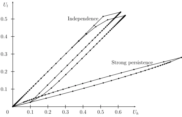
We now return to the general model in which types are persistent rather than independent.

As an initial exercise, consider the case of perfect persistence ρ

= ρ

= 0. If types never change, there is simply no possibility for the principal to use future allocations as an instrument to elicit truth-telling. We revert to the static problem for which the solution is to either always provide the good (if µ ≥ c) or never do so.

This case suggests that persistence plays an ambiguous role a priori. Because current types assign different probabilities of being (for example) high types tomorrow, one might hope that tying promised future utility to current reports might facilitate truth-telling. How- ever, the case of perfectly persistent types suggests that correlation diminishes the scope for using future allocations as “transfers.” Utilities might still be separable over time, but the

19

This result might be surprising given Cohn’s (2010) “improvement” upon Jackson and Sonnenschein.

However, while Jackson and Sonnenschein cover our set-up, Cohn does not and features more instruments

at the principal’s disposal. See also Eilat and Pauzner (2011) for an optimal mechanism in a related setting.

current type affects both flow and continuation utility. Definite comparative statics are obtained in the continuous time limit, see Section 5.1.

The techniques that served us well with independent values are no longer useful. We will not be able to rely on martingale techniques. Worse, ex ante utility is no longer a valid state variable. To understand why, note that with independent types, an agent of a given type can evaluate his continuation utility based only on current type, probabilities of trade as a function of his report, and promised utility tomorrow as a function of his report.

However, if today’s type is correlated with tomorrow’s type, how can the agent evaluate his continuation utility without knowing how the principal intends to implement it? This is problematic because the agent can deviate, unbeknown to the principal, in which case the continuation utility computed by the principal, given his incorrect belief regarding the agent’s type tomorrow, is not the same as the continuation utility under the agent’s belief.

However, conditional on the agent’s type tomorrow, his type today carries no information on future types by the Markovian assumption. Hence, tomorrow’s promised ex interim utilities suffice for the agent to compute his utility today regardless of whether he deviates;

that is, we must specify his promised utility tomorrow conditional on each possible report at that time. Of course, his type tomorrow is not observable. Hence, we must use the utility he receives from reporting his type tomorrow, conditional on truthful reporting. This creates no difficulty, as on path, the agent has an incentive to truthfully report his type tomorrow.

Hence, he does so after having lied during the previous round (conditional on his current type and his previous report, his previous type does not affect the decision problem he faces).

That is, the one-shot deviation principle holds here: when a player considers lying, there is

no loss in assuming that he will report truthfully tomorrow. Hence, the promised utility pair

that we use corresponds to his actual possible continuation utilities if he plays optimally in

the continuation regardless of whether he reports truthfully today. We are obviously not the

first to highlight the necessity of using as a state variable the vector of ex interim utilities,

given a report today, as opposed to the ex ante utility when types are serially correlated. See

Townsend (1982), Fernandes and Phelan (2000), Cole and Kocherlakota (2001), Doepke and

Townsend (2006) and Zhang and Zenios (2008). Hence, to use dynamic programming, we

must include as state variables the pair of utilities that must be delivered today as a function

of the report. Nevertheless, this is insufficient to evaluate the payoff to the principal. Given

such a pair of utilities, we must also specify his belief regarding the agent’s type. Let φ

denote the probability that he assigns the high type. This belief can take only three values

depending on whether this is the initial round or whether the previous report was high or

low. Nonetheless, we treat φ as an arbitrary element in the unit interval.

Another complication arises from the fact that the principal’s belief depends on the history. For this belief, the last report is sufficient.

4.1 The Program

As discussed above, the principal’s optimization program, cast as a dynamic programming problem, requires three state variables: the belief of the principal, φ = P [v = h] ∈ [0, 1], and the pair of (ex interim) utilities that the principal delivers as a function of the current report, U

, U

. The highest utility µ

(resp., µ

) that can be given to a player whose type is high (or low) delivered by always supplying the good solves

µ

= (1 − δ)h + δ(1 − ρ

)µ

+ δρ

µ

, µ

= (1 − δ)l + δ(1 − ρ

)µ

+ δρ

µ

; that is,

µ

= h − δρ

(h − l)

1 − δ + δ(ρ

+ ρ

) , µ

= l + δρ

(h − l) 1 − δ + δ(ρ

+ ρ

) . We note that

µ

− µ

= 1 − δ

1 − δ + δ(ρ

+ ρ

) (h − l).

The gap between the maximum utilities as a function of the type decreases in δ, vanishing as δ → 1.

A policy is now a pair (p

, p

) : R

→ [0, 1]

mapping the current utility vector U = (U

, U

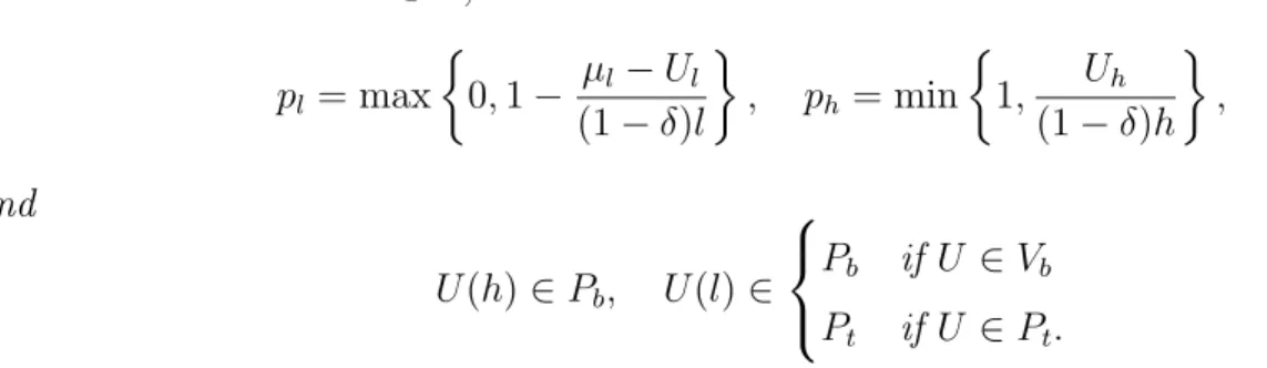
) onto the probability with which the good is supplied as a function of the report and a pair (U (h), U (l)) : R

→ R

mapping U onto the promised utilities (U

(h), U

(h)) if the report is h and (U

(l), U

(l)) if it is l. These definitions abuse notation, as the domain of (U (h), U (l)) should be those utility vectors that are feasible and incentive-compatible.

Define the function W : [0, µ

] × [0, µ

] × [0, 1] → R ∪ {−∞} that solves the following program for all U ∈ [0, µ

] × [0, µ

], and φ ∈ [0, 1]:

W (U, φ) = sup { φ ((1 − δ)p

(h − c) + δW (U (h), 1 − ρ

)) + (1 − φ) ((1 − δ)p

(l − c) + δW (U (l), ρ

)) } ,

over p

, p

∈ [0, 1], and U (h), U (l) ∈ [0, µ

] × [0, µ

] subject to promise keeping and incentive compatibility, namely,

U

= (1 − δ)p

h + δ(1 − ρ

)U

(h) + δρ

U

(h) (2)

≥ (1 − δ)p

h + δ(1 − ρ

)U

(l) + δρ

U

(l), (3)

and

U

= (1 − δ)p

l + δ(1 − ρ

)U

(l) + δρ

U

(l) (4)

≥ (1 − δ)p

l + δ(1 − ρ

)U

(h) + δρ

U

(h), (5) with the convention that sup W = −∞ whenever the feasible set is empty. Note that W is concave on its domain (by the linearity of the constraints in the promised utilities). An optimal policy is a map from (U, φ) into (p

, p

, U(h), U (l)) that achieves the supremum for some W .

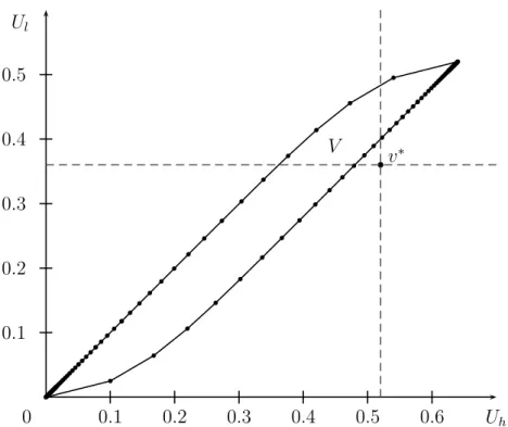
4.2 Complete Information

Proceeding as with independent values, we briefly derive the solution under complete infor- mation, that is, dropping (3) and (5). Write W ¯ for the resulting value function. Ignoring promises, the efficient policy is to supply the good if and only if the type is h. Let v

(resp., v

) denote the utility that a high (low) type obtains under this policy. The pair (v

, v

) satisfies

v

= (1 − δ)h + δ(1 − ρ

)v

+ δρ

v

, v

= δ(1 − ρ

)v

+ δρ

v

, which yields

v

= h(1 − δ(1 − ρ

))

1 − δ(1 − ρ

− ρ

) , v

= δhρ

1 − δ(1 − ρ

− ρ

) .

When a high type’s promised utility U

is in [0, v

], the principal supplies the good only if the type is high. Therefore, the payoff is U

(1 − c/h). When U

∈ (v

, µ

], the principal always supplies the good if the type is high. To fulfill the promised utility, the principal also produces the good when the agent’s type is low. The payoff is v

(1 − c/h)+(U

− v

)(1 − c/l).

We proceed analogously given U

(notice that the problems of delivering U

and U

are uncoupled). In summary, W ¯ (U, φ) is given by



 

 

 



 

 

 



φ

+ (1 − φ)

if U ∈ [0, v

] × [0, v

], φ

+ (1 − φ)

l(h−c)

h

+

if U ∈ [0, v

] × [v

, µ

], φ

h(h−c)

h

+

∗ h)(l−c) l

+ (1 − φ)

if U ∈ [v

, µ

] × [0, v

], φ

h(h−c)

h

+

+ (1 − φ)

h

+

if U ∈ [v

, µ

] × [v

, µ

].

For future purposes, note that the derivative of W (differentiable except at U

= v

and U

= v

) is in the interval [1 − c/l, 1 − c/h], as expected. The latter corresponds to the most efficient utility allocation, whereas the former corresponds to the most inefficient allocation.

In fact, W is piecewise linear (a “tilted pyramid”) with a global maximum at v

= (v

, v

).

4.3 Feasible and Incentive-Feasible Payoffs

One difficulty in using ex interim utilities as state variables rather than ex ante utility is that the dimensionality of the problem increases with the cardinality of the type set. Another related difficulty is that it is not obvious which vectors of utilities are feasible given the incentive constraints. Promising to assign all future units to the agent in the event that his current report is high while assigning none if this report is low is simply not incentive compatible.

The set of feasible utility pairs (that is, the largest bounded set of vectors U such that (2) and (4) can be satisfied with continuation vectors in the set itself) is easy to describe.

Because the two promise keeping equations are uncoupled, it is simply the set [0, µ

] × [0, µ

] itself (as was already implicit in Section 4.2).

What is challenging is to solve for the incentive-compatible, feasible (in short, incentive- feasible) utility pairs: these are ex interim utilities for which we can find probabilities and pairs of promised utilities tomorrow that make it optimal for the agent to report his value truthfully such that these promised utility pairs tomorrow satisfy the same property.

Definition 1 The incentive-feasible set, V ∈ R

, is the set of ex interim utilities in round 0 that are obtained for some incentive-compatible policy.

It is standard to show that V is the largest bounded set such that for each U ∈ V there exists p

, p

∈ [0, 1] and two pairs U (h), U (l) ∈ V solving (2)–(5).

Our first step toward solving for the optimal mechanism is to solve for V . To obtain some intuition regarding its structure, let us review some of its elements. Clearly, 0 ∈ V, µ :=

(µ

, µ

) ∈ V . It suffices to never or always supply the unit, independent of the reports, which is incentive compatible.

More generally, for some integer m ≥ 0, the principal can supply the unit for the first m rounds, independent of the reports, and never supply the unit after. We refer to such policies as pure frontloaded policies because they deliver a given number of units as quickly as possible. More generally, a (possibly mixed) frontloaded policy is one that randomizes over two pure frontloaded policies with consecutive integers m, m+ 1.

20

Clearly, incentive-feasibility is closely related to self-generation (see Abreu, Pearce and Stacchetti, 1990), though it pertains to the different types of a single agent rather than to different players in the game. The distinction is not merely a matter of interpretation because a high type can become a low type and vice- versa, which represents a situation with no analogue in repeated games. Nonetheless, the proof of this characterization is identical.

21

With some abuse, we write µ ∈ R

, as it is the natural extension as an upper bound of the feasible set

of µ ∈ R .

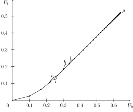
Similarly, we define a pure backloaded policy as one that does not supply the good for the first m rounds but does afterward, independent of the reports. (Mixed backloaded policies being defined in the obvious way.)

Suppose that we fix a backloaded and a frontloaded policy such that the high-value agent is indifferent between the two. Then, the low-value agent surely prefers the backloaded policy.

The backloaded policy affords him “more time” to switch from his (initial) low value to a high value. Hence, given U

∈ (0, µ

), the utility U

obtained by the backloaded policy that awards U

to the high type is higher than the utility U

of the frontloaded policy that also yields U

.

The utility pairs corresponding to backloading and frontloading are easily solved because they obey simple recursions. First, for ν ≥ 0, let

u

= δ

µ

− δ

(1 − q)(µ

− µ

)(1 − κ

), (6) u

= δ

µ

+ δ

q(µ

− µ

)(1 − κ

), (7) and set u

:= (u

, u

). Second, for ν ≥ 0, let

u

= (1 − δ

)µ

+ δ

(1 − q)(µ

− µ

)(1 − κ

), (8) u

= (1 − δ

)µ

− δ

q(µ

− µ

)(1 − κ

), (9) and set u

:= (u

, u

). The sequence u

is decreasing (in both its arguments) as ν in- creases, with u

= µ and with lim

u

= 0. Similarly, u

is increasing, with u

= 0 and lim

u

= µ.

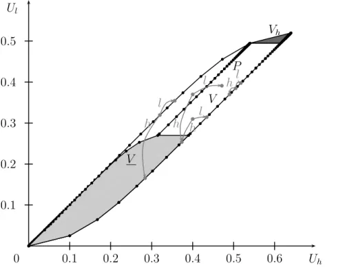
Backloading not only is better than frontloading for the low-value agent but also fixes the high-value agent’s utility. These policies yield the best and worst utilities. Formally, Lemma 5 It holds that

V = co { u

, u

: ν ≥ 0 } .

That is, V is a polygon with a countable infinity of vertices (and two accumulation points).

See Figure 2 for an illustration. It is easily verified that

ν

lim

u

− u

u

− u

= lim

ν→∞

u

− u

u

− u

= 1.

When the switching time ν is large, the change in utility from increasing this time has an

impact on the agent’s utility that is essentially independent of his initial type. Hence, the

slopes of the boundaries are less than 1 and approach 1 as ν → ∞ . Because (µ

− v

)/(µ

−

U

U

0 0.1 0.2 0.3 0.4 0.5 0.6

0.1 0.2 0.3 0.4

0.5

b

b

b

b

b

b

b

b

b

b

b

b

b

b

b

bbbbbbbbbbbbbbbbbbbbbbb

b b

bb b b b b b b b b b b b b b b b b bbbbbbbbbbb bb bb bb b bb b

b

V

b

v

Figure 2: The set V for parameters (δ, ρ

, ρ

, l, h) = (9/10, 1/3, 1/4, 1/4, 1).

v

) > 1, the vector v

is outside V . For any φ, the complete-information value function W ¯ (U, φ) increases as we vary U within V toward its lower boundary, either horizontally or vertically. This pattern should not be particularly surprising. Due to private information, the low-type agent derives information rents such that if the high-type agent’s utility were first-best, the low-type agent’s utility would be too high. It is instructive to study how the shape of V varies with persistence. When κ = 0 and values are independent over time, the lower type agent prefers to receive a larger fraction (or probability) of the good tomorrow rather than today (adjusting for discounting) but has no preference over later times. The case is analogous for the high type agent. As a result, all the vertices { u

}

(resp., { u

}

) are aligned and V is a parallelogram with vertices 0, µ, u

and u

. As κ increases, the imbalance between type utilities increases and the set V flattens. In the limit of perfect persistence, the low-type agent no longer feels differently about frontloading vs. backloading because no amount of time allows his type to change. See Figure 3.

The structure of V relies on the assumption κ ≥ 0. If types were negatively correlated

over time, then frontloading and backloading would not be policies spanning the boundary

of V . This fact is easily seen by considering the case in which there is perfect negative serial

correlation. Then, providing the unit if only if the round is odd (even) favors (hurts) the low-