Lecture 4
Fault-Tolerant Clock Synchronization
In the previous lectures, we assumed that the world is a happy place without any kind of faults. This is not a realistic assumption in large-scale systems, and it is an issue in high reliability systems as well. After all, if the system clock fails, there may be no further computations at all!
As, in general, it is difficult to predict what kind of faults may happen, again we assume a worst-case model: Failing nodes may behave in any conceivable manner, including collusion, predicting the future, sending conflicting informa- tion to di↵erent nodes, or even pretending to be correct nodes (for a while). In other words, the system should still function no matter what kind of faults may occur. This may be overly pessimistic in the sense that “real” faults might have a very hard time to produce such behavior. However, if we can handle all of these possibilities, we’re on the safe side in that we do not have to study what kind of faults may actually happen and verify the resulting fault model(s) for each and every system we build.
Definition 4.1 (Byzantine Faults). A Byzantine faulty node may behave arbi- trarily, i.e., it does not follow any algorithm described by the system designer.
The set of faulty nodes is (initially) unknown to the other nodes. In other words, the algorithm must be designed in such a way that it works correctly regardless of which nodes are faulty. “Working correctly” here means that all requirements and guarantees on clocks, skews, etc. need only be satisfied by the set V
gof nodes that are not faulty.
Unsurprisingly, such a strong fault model results in limitations on what can be achieved. For instance, if more than half of the nodes in the system are faulty, there is no way to achieve any kind of synchronization. In fact, even if half of the neighbors of some node are faulty, this is impossible. The intuition is simple: Split the neighborhood of some node v in two sets A and B and consider two executions, E
Aand E
B, such that A is faulty in E
Aand B is faulty in E
B. Given that A is faulty in E
A, B and v need to stay synchronized in E
A, regardless of what the nodes in A do. However, the same applies to E
Bwith the roles of A and B reversed. However, A and B can have di↵erent opinions on the time, and v has no way of figuring out which set to trust.
37
In fact, it turns out that the number f of faulty nodes must satisfy 3f < n or no solution is possible (without cryptographic assumptions); we show this later. Motivated by the above considerations, we also confine ourselves to G being a complete graph: each node is connected to each other node, i.e., each pair of nodes can communicate directly.
4.1 The Pulse Synchronization Problem
Let’s study a simpler version of the clock synchronization problem, which we call pulse synchronization. Instead of outputting a logical clock at all times, nodes merely need to jointly generate roughly synchronized pulses whose frequency is bounded from above and below.
Definition 4.2 (Pulse Synchronization). Each (non-faulty) node is to generate each pulse i 2 N exactly once. Denoting by p
v,ithe time when node v generates pulse i, we require that there are S , P
min, P
max2 R
+so that
• max
i2N,v,w2Vg{| p
v,ip
w,i|} S (skew)
• min
i2N{ min
v2Vg{ p
v,i+1} max
v2Vg{ p
v,i}} P
min(minimum period)
• max
i2N{ max
v2Vg{ p
v,i+1} min
v2Vg{ p
v,i}} P
max(maximum period) Remarks:
• The idea is to interpret the pulses as the “ticks” of a common clock.
• Ideally, S is as small as possible, while P
minand P
maxare as close to each other as possible and can be scaled freely.
• Due to the lower bound from Lecture 1, we have that S u/2.
• Clearly, we cannot expect better than P
max#P
min, i.e., matching the quality of the hardware clocks. Also, P
maxP
minS .
• Because D = 1, the problem would be trivial without faults. For instance, the Max Algorithm would achieve skew u + (# 1)(d + T), and pulses could be triggered every ⇥( G ) local time.
• The difficulty lies in preventing the faulty nodes from dividing the correctly functioning nodes into unsynchronized subsets.
4.2 A Variant of the Srikanth-Toueg Algorithm
One of our design goals here is to keep the algorithm extremely simple. To this end, we decide that
• Nodes will communicate by broadcast (i.e., sending the same information to all other nodes, for simplicity including themselves) only. Note that faulty nodes do not need to stick to this rule!
• Messages are going to be very short. In fact, there is only a single type
of message, carrying the information that a node transitioned to state
propose.
• Nodes will store, for each node, whether they received such a message.
On some state transitions, they will reset these memory flags to 0 (i.e., no message received yet).
• Not accounting for the memory flags, each node runs a state machine with a constant number of states.
• Transitions in this state machine are triggered by expressions involving (i) the own state, (ii) thresholds for the number of memory flags that are 1, and (iii) timeouts. A timeout means that a node waits for a certain amount of local time after entering a state before considering a timeout expired, i.e., evaluating the respective expression to true. The only exception is the starting state reset, from which nodes transition to start when the local clock reaches H
0, where we assume that max
v2Vg{ H
v(0) } < H
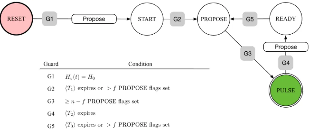
0. The algorithm, from the perspective of a node, is depicted in Figure 4.1. The idea is to repeat the following cycle:
• At the beginning of an iteration, all nodes transition to state ready (or, initially, start) within a bounded time span. This resets the flags.
G1
G3 G2
Guard Condition
G4
G5 hT3iexpires or > fPROPOSE flags set hT1iexpires or > fPROPOSE flags set
hT2iexpires
n fPROPOSE flags set Hv(t) =H0
RESET START PROPOSE READY
PULSE Propose Propose
G3 G2
G1 G5
G4
Figure 4.1: State machine of a node in the pulse synchronisation algorithm.
State transitions occur when the condition of the guard in the respective edge
is satisfied (gray boxes). All transition guards involve checking whether a local
timer expires or a node has received propose messages from sufficiently many
di↵erent nodes. The only communication is that a node broadcasts to all nodes
(including itself) when it transitions to propose. The notation h T i evaluates
to true when T time units have passed on the local clock since the transition to
the current state. The boxes labeled propose indicates that a node clears its
propose memory flags when transitioning from reset to start and pulse to
ready. That is, the node forgets who it has “seen” in propose at some point
in the previous iteration. All nodes initialize their state machine to state reset,
which they leave at the time t when H
v(t) = H
0. Whenever a node transitions
to state pulse, it generates a pulse. The constraints imposed on the timeouts
are listed in Inequalities (4.1)–(4.4).
• Nodes wait in this state until they are sure that all correct nodes reached it. Then, when a local timeout expires, they transition to propose.
• When it looks like all correct nodes (may) have arrived there, they transi- tion to pulse. As the faulty nodes may never send a message, this means to wait for n f nodes having announced to be in propose.
• However, faulty nodes may also sent propose messages, meaning that the threshold is reached despite some nodes still waiting in ready for their timeouts to expire. To “pull” such stragglers along, nodes will also transition to propose if more than f of their memory flags are set. This is proof that at least one correct node transitioned to propose due to its timeout expiring, so no “early” transitions are caused by this rule.
• Thus, if any node hits the n f threshold, no more than d time later each node will hit the f + 1 threshold. Another d time later all nodes hit the n f threshold, i.e., the algorithm has skew 2d.
• The nodes wait in pulse sufficiently long to ensure that no propose mes- sages are in transit any more before transitioning to ready and starting the next iteration.
For this reasoning to work out, a number of timing constraints need to be satisfied:
H
0> max
v2Vg
{ H
v(0) } (4.1)
T
1# H
0(4.2)
T
2# 3d (4.3)
T
3#
✓
1 1
#
◆
T
2+ 2d (4.4)
Lemma 4.3. Suppose 3f < n and the above constraints are satisfied. Moreover, assume that each v 2 V
gtransitions to start (ready) at a time t
v2 [t , t], no such node transitions to propose during (t d, t
v), and T
1# (T
3# ). Then there is a time t
02 (t + T
1/#, t + T
1d) (t
02 (t + T
3/#, t + T
3d)) such that each v 2 V
gtransitions to pulse during [t
0, t
0+ 2d).
Proof. We perform the proof for the case of start and T
1; the other case is analogous. Denote by t
pthe smallest time larger than t d when some v 2 V
gtransitions to propose (such a time exists, as T
1will expire if a node does not transition to propose before this happens). By assumption and the definition of t
p, no v 2 V
gtransitions to propose during (t d, t
p), implying that no node receives a message from any such node during [t , t
p]. As v 2 V
gclears its memory flags when transitioning to ready at time t
vt , this implies that the node(s) from V
gthat transition to propose at time t
pdo so because T
1expired. As hardware clocks run at most at rate # and for each v 2 V
git holds that t
vt , it follows that
t
pt + T
1# t .
Thus, at time t
pt, each v 2 V
ghas reached state ready and will not reset its memory flags again without transitioning to pulse first.
From this observation we can infer that each v 2 V
gwill transition to pulse:
Each v 2 V
gtransitions to propose during [t
p, t+ T
1], as it does so at the latest at time t
v+ T
1 t + T
1due to T
1expiring. Thus, by time t + T
1+ d each v 2 V
greceived the respective messages and, as | V
g| n f , transitioned to pulse.
It remains to show that all correct nodes transition to pulse within 2d time.
Let t
0be the minimum time after t
pwhen some v 2 V
gtransitions to pulse. If t
0t + T
1d, the claim is immediate from the above observations. Otherwise, note that out of the n f of v’s flags that are true, at least n 2f > f correspond to nodes in V
g. The messages causing them to be set have been sent at or after time t
p, as we already established that any flags that were raised earlier have been cleared before time t t
p. Their senders have broadcasted their transition to propose to all nodes, so any w 2 V
ghas more than f flags raised by time t
0+ d, where d accounts for the potentially di↵erent travelling times of the respective messages. Hence, each w 2 V
gtransitions to propose before time t
0+ d, the respective messages are received before time t
0+ 2d, and, as | V
g| n f , each w 2 V
gtransitions to pulse during [t
0, t
0+ 2d).
Theorem 4.4. Suppose that 3f < n and the above constraints are satisfied.
Then the algorithm given in Figure 4.1 solves the pulse synchronization problem with S = 2d, P
min= (T
2+ T
3)/# 2d and P
max= T
2+ T
3+ 3d.
Proof. We prove the claim by induction on the pulse number. For each pulse, we invoke Lemma 4.3. The first time, we use that all nodes start with hardware clock values in the range [0, H
0) by (4.1). As hardware clocks run at least at rate 1, thus all nodes transition to state start by time H
0. By (4.2), the lemma can be applied with t = = H
0, yielding times p
v,1, v 2 V
g, satisfying the claimed skew bound of 2d.
For the induction step from i to i + 1, (4.3) yields that v 2 V
gtransitions to ready no earlier than time
p
v,i+ T
2# max
w2Vg
{ p
w,i} + T
2# 2d max
w2Vg
{ p
w,i} + d and no later than time
p
v,i+ T
2 max
w2Vg
{ p
w,i} + T
2.
Thus, by (4.4) we can apply Lemma 4.3 with t = max
w2Vg{ p
w,i} + T
2and
= (1 1/#)T
2+ 2d, yielding pulse times p
v,i+1, v 2 V
g, satisfying the stated skew bound.
It remains to show that min
v2Vg{ p
v,i+1} max
v2Vg{ p
v,i} (T
2+T
3)/# 2d and max
v2Vg{ p
v,i+1} min
v2Vg{ p
v,i} T
2+ T
3+ 3d. By Lemma 4.3,
p
v,i+12
✓
t + T
3# , t + T
3+ d
◆
=
✓
w
max
2Vg{ p
w,i} + T
2+ T
3# 2d, max
w2Vg