Visual Robot Navigation with Omnidirectional Vision
From Local and Map-Based Navigation to Semantic Navigation
DISSERTATION
submitted in partial fulfillment of the requirements for the degree
Doktor Ingenieur (Doctor of Engineering)
in the
Faculty of Electrical Engineering and Information Technology TU Dortmund University
by
Luis Felipe Posada Medellin, Colombia
Date of submission: 29th August 2018
First examiner: Univ.-Prof. Dr.-Ing. Prof. h.c. Dr. h.c. Torsten Bertram Second examiner: Univ.-Prof. Dr.-Ing Ralf Mikut
Date of approval: 1st October 2019
"Dedicated to the memory of my father."
Acknowledgments
This thesis means the closing of the dream of studying in Germany that I built since I was a child. The stories I heard from my great-grandparents, German engineers who emigrated to Colombia in the 19th century to work in the gold mines of Titiribí, awakened in me great curiosity about Germany. But perhaps the strongest latent force that pushed me on this journey came from my father, Héctor Posada, an engineer at MIT and a pioneer in Latin America in computer science and telecommunications.
Unfortunately, the violent conflict of the ’90s in Colombia took his life, but his exam- ple, tenacity, and wit would remain within me and later would become my greatest inspiration to study abroad. In honor of him, I dedicate this thesis.
This work would not have been possible without Prof. Dr.-Ing. Prof. h.c. Dr.
h.c. Torsten Bertram, who gave me the chance to work as a member of the RST department and inspired me with his leadership and professionalism. I am grateful to apl. Prof. Dr. rer. nat. Frank Hoffmann, who introduced me to new exciting topics and fueled me with ideas. A significant part of this thesis is due to his in-depth technical knowledge and advice he so kindly offered me. I extend my thanks to Prof.
Dr.-Ing Ralf Mikut, who kindly agreed to review this work as the second examiner.
I am very grateful to all RST colleagues with whom I have worked. Especially Kr- ishna Narayananan and Javier Oliva. Krishna accompanied me from day one, giving me support and feeding me with enriching discussions and suggestions. Javier be- came one of the most inspiring people I met in Germany. In addition to offering me a great friendship, he taught me how to reach millions of people through the Internet.
I am also thankful to Thomas Nierobisch, who was my master thesis advisor and en- couraged me to continue my doctoral studies at RST, to Jürgen Limhoff for helping us with the robotic platform and hardware, and to Mareike Leber and Gabriele Rebbe for their endless help the paperwork which made our work more comfortable. I extend my gratitude to other RST members, students, and friends who, unfortunately, due to space, I cannot mention, but offered me help and feedback.
I am very thankful to Colciencias for giving me financial support through the "Fran- cisco José de Caldas" scholarship and the NRW state for a semester scholarship during the early days of this thesis.
I am forever grateful to my mother, Amalia, who was the person that supported me the most through the distance in all aspects during my stay in Germany; also, my siblings Soledad and Camilo for being always there for me, whenever I needed them.
Finally, the last words of gratitude are for my partner Melissa for her love, unlimited
support, patience, and life knowledge.
Abstract
In a world where service robots are increasingly becoming an inherent part of our lives, it has become essential to provide robots with superior perception capabilities and acute semantic knowledge of the environment. In recent years, the computer vision field has advanced immensely, providing rich information at a fraction of the cost. It has thereby become an essential part of many autonomous systems and the sensor of choice while tackling the most challenging perception problems. Nevertheless, it is still challenging for a robot to extract meaningful information from an image signal (a high dimensional, complex, and noisy data). This dissertation presents several contributions towards visual robot navigation relying solely on omnidirectional vision.
The first part of the thesis is devoted to robust free-space detection using omnidirec- tional images. By mimicking a range sensor, the free-space extraction in the omniview constitutes a fundamental block in our system, allowing for collision-free navigation, localization, and map-building. The uncertainty in the free-space classifications is han- dled with fuzzy preference structures, which explicitly expresses it in terms of prefer- ence, conflict, and ignorance. This way, we show it is possible to substantially reduce the classification error by rejecting queries associated with a strong degree of conflict and ignorance.
The motivation of using vision in contrast to classical proximity sensors becomes apparent after the incorporation of more semantic categories in the scene segmenta- tion. We propose a multi-cue classifier able to distinguish between the classes: floor, vertical structures, and clutter. This result is further enhanced to extract the scene’s spa- tial layout and surface reconstruction for a better spatial and context awareness. Our scheme corrects the problematic distortions induced by the hyperbolic mirror with a novel bird’s eye formulation. The proposed framework is suitable for self-supervised learning from 3D point cloud data.
Place context is integrated into the system by training a place category classifier able to distinguish among the categories: room, corridor, doorway, and open space. Hand engineered features, as well as those learned from data representations, are considered with different ensemble systems.
The last part of the thesis is concerned with local and map-based navigation. Several visual local semantic behaviors are derived by fusing the semantic scene segmentation with the semantic place context. The advantage of the proposed local navigation is that the system can recover from conflicting errors while activating behaviors in the wrong context. Higher-level behaviors can also be achieved by compositions of the basic ones.
Finally, we propose different visual map-based navigation alternatives that reproduce
or achieve better results compared to classical proximity sensors, which include: map
generation, particle filter localization, and semantic map building.
Contents
1 Introduction 1
1.1 Experimental Platform . . . . 2
1.2 Contributions and Outline . . . . 2
2 Visual Range Sensor 6 2.1 Introduction . . . . 6
2.2 Related Work . . . . 7
2.3 Free-Space Detection with Ensemble of Experts . . . . 8
2.3.1 System Architecture . . . . 8
2.3.2 Segmentation and Features . . . . 10
2.3.3 Experimental Results . . . . 15
2.4 Online Self-Supervised Free-Space with Range Image Data . . . . 17
2.4.1 System Architecture . . . . 17
2.4.2 Validation Data with a Range Camera . . . . 18
2.4.3 Experimental Results . . . . 20
2.5 Summary . . . . 22
3 Uncertainty Representation with Fuzzy Preference Structures 23 3.1 Introduction . . . . 23
3.2 Related Work . . . . 24
3.3 Fuzzy Preference Structures . . . . 24
3.3.1 Preference Structure and Classification . . . . 25
3.3.2 Valued Preferences for Ensembles of Segmentations . . . . 27
3.3.3 Experimental Results: Classification of Indoor Scenarios . . . . . 27
3.4 Ensemble of Experts with Fuzzy Preference Structures . . . . 31
3.4.1 Classification Results . . . . 31
3.5 Summary . . . . 35
4 Semantic Segmentation of Scenes 36 4.1 Introduction . . . . 36
4.2 Related Work . . . . 37
4.3 Semantic Segmentation . . . . 38
4.4 Features . . . . 38
4.4.1 Location . . . . 38
4.4.2 Color . . . . 39
4.4.3 Local Intensity Distribution . . . . 39
4.4.4 Shape . . . . 40
4.4.5 Texture . . . . 43
4.5 Random Forest Classification . . . . 43
4.6 Semantic Segmentation Results . . . . 44
4.7 Self-Supervised Semantic Segmentation with Range Images . . . . 48
4.8 Summary . . . . 48
5 Surface Layout of Scenes 49 5.1 Introduction . . . . 49
5.2 Related Work . . . . 50
5.3 Surface Layout Approach . . . . 51
5.3.1 Free-space and Vertical Structures . . . . 51
5.3.2 Vanishing Points Estimation and Oriented Lines . . . . 52
5.3.3 Floor-Wall Boundary Features . . . . 55
5.3.4 Histogram of Oriented Gradients . . . . 56
5.4 Experimental Results . . . . 57
5.5 Summary . . . . 58
6 Visual Place Category Recognition 60 6.1 Introduction . . . . 60
6.2 Related Work . . . . 61
6.3 System Architecture . . . . 62
6.4 Engineered Visual Features . . . . 62
6.4.1 Gradient-Based Features . . . . 63
6.4.2 Texture-Based Features . . . . 64
6.4.3 Color-Based Features . . . . 64
6.4.4 Shape-Based Features . . . . 64
6.5 Learned Visual Features . . . . 65
6.6 Classification . . . . 66
6.6.1 Support Vector Machines . . . . 67
6.7 Place Recognition Results . . . . 70
6.8 Summary . . . . 72
7 Behavior-Based Local Semantic Navigation 77 7.1 Introduction . . . . 77
7.2 Related Work . . . . 78
7.3 System Architecture . . . . 79
7.4 Semantic Segmentation . . . . 80
7.5 Door Detection . . . . 80
7.6 Navigation Behaviors . . . . 81
7.6.1 Goal Point Homing . . . . 81
7.6.2 Corridor Centering . . . . 82
7.6.3 Obstacle Avoidance . . . . 83
7.6.4 Door Passing Behavior . . . . 85
7.6.5 High-Level Behaviors . . . . 87
7.7 Summary . . . . 87
8 Map-Based Navigation and Semantic Mapping 88
8.1 Introduction . . . . 88
8.2 Related Work . . . . 89
8.3 Semantic Mapping Framework . . . . 90
8.3.1 Free Space Segmentation . . . . 90
8.3.2 Inverse Sensor Model . . . . 92
8.3.3 Occupancy Grid Mapping . . . . 92
8.3.4 Place Classification . . . . 93
8.3.5 Semantic Mapping . . . . 93
8.4 Semantic Mapping Results . . . . 94
8.5 Monte Carlo Localization with Omnidirectional Vision . . . . 95
8.6 Robot Localization Results . . . . 99
8.7 Summary . . . . 99
9 Conclusions and Outlook 101 Bibliography 103 Published Papers . . . 103
Contributed Papers . . . 104
References . . . 105
1
Introduction
Robots are migrating faster and faster from typical industrial applications to human environments to perform increasingly complex tasks. This transition requires higher perception capabilities and intelligence. Conventionally, mobile robots have operated using range sensors, which provide robust proximity information to nearby obstacles.
However, in recent years, vision has emerged as a more versatile alternative as it pro- vides more information, albeit more complex. This development is further supported by the increasing availability of powerful computer vision systems at affordable costs.
Inspired by the human vision, our most important sensor, we expect the robot of the future to have a deep semantic understanding of the world to dramatically improve human-robot natural communication, navigation, localization, and recognition of sur- rounding objects. Nevertheless, despite the recent advances, it is still challenging for a robot to extract meaningful information from the image signal (a high dimensional, complex, and noisy data), since:
• Navigation relies on depth information of the scene, which is not provided by a single 2D image.
• Raw image data is rather complex, which implies the need to segment and group objects to extract their relevant features and to aggregate those in a meaningful manner.
• Visual cues such as intensity, texture, and optical flow are highly context-depen- dent.
• Visual appearance of the environment and objects vary substantially with view- point and illumination.
This dissertation focuses on the visual navigation of mobile robots solely through omnidirectional vision. We investigate different aspects of visual navigation, provid- ing the robot with the following capabilities: (i) deriving the free-space in the scene for collision-free navigation, (ii) handling uncertainty in the free-space classification for improving the robot’s decision making, (iii) gaining semantic knowledge through clas- sification of image regions, (iv) improving the spatial understanding through layout and structure recovery, (v) advancing place recognition for context-aware navigation, (vi) enhancing local semantic navigation with visual behaviors, and (vii) building a semantic mapping and achieving a purely visual map-based navigation.
Specifically, our work is concerned with omnidirectional-vision, which provides
a wide field-of-view or panoramic snapshot of the environment. The advantage of
1 Introduction
an omni-view (similar to a laser rangefinder), is that it captures the environment around 360 ◦ invariant under rotation. Additionally, the appearance variation between consecutive frames is small, given the low optical-flow due to the wide field-of-view which is beneficial for navigation, map building, and localization. These advantages come with the cost of low resolution, high distortion, and a blind-spot in the image due to the nature of the hyperbolic mirrors. These limitations can be overcome, as we shall see in the contributions derived in the following chapters.
1.1 Experimental Platform
The experimental platform used throughout this work consists of a Pioneer 3DX mo- bile robot shown in Fig. 1.1. The robot is equipped with a range camera and an omnidirectional camera.
Omnicamera
Range Camera
Omni-image
RGB image Range image Pioneer Robot
Kinect
PMD Laser
rangefinder
Ultrasonic sensors
Figure 1.1: Robotic Platform and sensors.
In the experiments conducted in the first two chapters, we employ a Photo-mixer Device Camera (PMD) as the 3D camera. The PMD provides 3D measurements at a 204 x 204 pixel resolution across a 40 ◦ x 40 ◦ field of view. In the latter chapters, the 3D data is acquired with a Microsoft Kinect, which provides 320 x 240 depth data across a 57 ◦ x 43 ◦ field of view. The omnidirectional sensor combines a CCD camera with a hyperbolic mirror that has a vertical field of view of 75 ◦ that is directed towards the bottom to capture the floor. Fig 1.2 illustrates at the right an omnidirectional image captured on the scene at the left. The robot was positioned on the corridor and objects on both images are labeled to illustrate how the hyperbolic mirror distorts the image, but is able to capture a 360 ◦ wide field of view. The robot is also outfitted with a SICK LMS-200 laser rangefinder and 16 Polaroid ultrasonic range sensors. The range data acquired with these proximity sensors are mainly used for validation.
1.2 Contributions and Outline
The organization of the thesis is outlined in Fig 1.3. The first chapters deal with
estimating the free-space in omnidirectional images. These chapters constitute a sig-
1.2 Contributions and Outline
Door
Floor Column
Extinguisher Posters
Door
Wall
Floor Colu
mn
Ex tin
gu ish
er
Posters
Door
Wall Door
Figure 1.2: Experimental platform positioned on a scene where the omnidirectional image at the right was captured. The scene and the omnidirectional image are labeled with the same objects to show the wide field of view image formation and distortion introduced by the hyperbolic mirror
nificant building block towards performing a purely visual local navigation and map building without relying on range from proximity sensors. From Chapter 4 onwards, the system incorporates more and more semantic understanding to take full advan- tage of the vision-based systems necessary to achieve more complex robotics tasks.
The outline of the thesis is as follows:
Chapter 2 introduces two novel free-space segmentation approaches for omnidi- rectional images that are pivotal for local navigation and map building in the last chapters. The first scheme rests upon the fusion of multiple classifications generated from heterogeneous segmentation schemes using a mixture of experts approach. The second scheme employs an online self-supervised scheme that selects the traversable floor region using the optimal segmentation to the appearance of the local environ- ment by cross-validation over 3D scans captured by a 3D range camera.
Chapter 3 investigates the uncertainty inherent in a single free-space segmentation as well as the global uncertainty across multiple segmentation based classifiers. The uncertainty of the classifications is explicitly expressed in terms of preference, conflict, and ignorance utilizing fuzzy preference structures, thereby mapping the problem of classification into the domain of decision-making under fuzzy preferences. We show that the classification error is substantially reduced by rejecting those queries associated with a strong degree of conflict and ignorance.
Chapter 4 extends the binary classifier from Chapter 2, increasing the number of semantic labels for each classified image’s region. The labeling distinguishes between the main classes: floor, vertical structures, and clutter. Vertical planes are objects such as walls, boards, and placards. Non-planar objects in the scene are grouped into the class clutter and are objects with multiple surfaces such as furniture, plants, people, or obstacles. We show that the method is suitable for self-supervised learning using the 3D point cloud data of a range camera.
Chapter 5 extends further the semantic segmentation by extracting the spatial lay-
out and surface reconstruction of the omnidirectional image. Knowing the spatial
layout of the scene improves scene understanding and enhances object detection. The
1 Introduction
proposed system benefits from a cascaded classification, where all vertical structures from the semantic segmentation are analyzed to find their main orientation by fusing orientation features from the HOG transform, floor/wall boundaries, and oriented lines in the image.
Chapter 6 presents a place-category recognition system that distinguishes among the location categories: room, corridor, doorway, and open space. The approach eval- uates hand-engineered features compared to learned-from-data representations. Dif- ferent combinations of heterogeneous features are tested with non-learning ensembles and ensembles that learn the model with supervised learning. The developed place recognition system is a fundamental block for the local semantic navigation and the semantic map building in Chapters 7 and 8.
Chapter 7 introduces a local semantic navigation approach based on visual behav- iors solely relying on omnidirectional vision. Four basic behaviors are presented:
goal point homing, corridor centering, obstacle avoidance, and door passing. Places in the behavior are described with a semantic category (e.g. room, corridor), while regions in the scene are also labeled with semantic regions (e.g. door, wall, floor). The proposed local navigation has the advantage that it can recover from conflicts, such as activating behaviors in the wrong context. The chapter also shows how to derive high-level behaviors by compositions of basic behaviors.
Chapter 8 deals with two aspects of the map-based navigation solely using om- nidirectional vision: (i) map localization, and (ii) semantic map building. The map representation consists of an occupancy grid constructed by a sensor model and its inverse from the segmented local robot’s free-space. The sensor model corrects the non-linear distortions of the omnidirectional mirror and outputs a scaled perspective image of the ground plane using a bird’s eye mapping. The free-space bird’s eye view images constitute the perceptual basis for both the mapping and the localiza- tion. Robot localization is achieved with the Monte Carlo method and the semantic map building uses the place category classifier from Chapter 6 to label categories:
room, corridor, doorway, and open room. Each place class maintains a separate grid
map that is fused with the range-based occupancy grid for building a dense semantic
map.
1.2 Contributions and Outline
Chapter 2: Visual Range Sensor
Image Free-space
Chapter 3: Uncertainty Representation
Preference
Ignorance
Conflict Image
Chapter 8: Map Based Navigation
Image
Semantic map
Behaviors
Chapter 6: Place Category Recognition
Image
Room Corridor Doorway Open space
Place
Chapter 7: Local Semantic Navigation Chapter 4: Semantic Segmentation
Floor Vertical Clutter Label
Image Semantic
segmentation
Chapter 5: Spatial Layout
Label
z-axis x-axis
y-axis
Image Surface
layout
Figure 1.3: Organization of the thesis
2
Visual Range Sensor
2.1 Introduction
Navigation is one of the fundamental skills a mobile robot should master to perform its task autonomously. Robot navigation has conventionally relied on range sensors that provide robust proximity information to nearby obstacles. However, in recent years, vision has emerged as an alternative, providing more information albeit more complex.
Vision, in contrast to range sensors, enables the appearance-based distinction of ob- jects, making it possible to differentiate, for example, ground floor, obstacles, people, walls, corridors, and doors. Notwithstanding, in spite of a large amount of informa- tion in an image, pure autonomous visual navigation remains a challenge given its noisy, high-dimensional, and complex data in its signal.
Free-space detection constitutes a significant building block for vision-based robot- ics as it supports high-level tasks such as localization, navigation, and map building.
In the context of mapless navigation, the segmentation of the free space in the local environment replaces or augments proximity sensors and supports a direct mapping from visual cues onto actions characteristic for reactive behaviors like in [Nar+09].
In this chapter, we address the problem of extracting free-space by segmenting the floor obstacle regions in omnidirectional images using two approaches. The first tech- nique rests upon the fusion of multiple classifications generated from heterogeneous segmentation schemes. Each segmentation relies on different features and cues to de- termine a pixel’s class label. The second approach extracts the traversable floor region in the omnidirectional robocentric view by selecting the segmentation optimal to the appearance of the local environment by cross-validation over 3D scans captured by 3D range camera.
While the literature reports several robust floor-obstacle segmentation methods, the novelty of our method lies in the following ideas: Use of the mixture of experts ap- proach [Pol06]. The key idea is to combine multiple segmentations in a way that the overall decision making benefits from the mutual competences of heterogeneous in- dividual classifiers. The analysis confirms that the combination of diverse classifiers achieves a classification rate that far exceeds the performance of any single classifier.
Additionally, our approach differs in several important aspects, namely: a) 3D range
camera instead of a laser scanner; b) segmentation of the range image in addition to
the 2D image; c) multiple representations of the appearance-based floor model; d)
2.2 Related Work various segmentation algorithms rather than one; e) obstacle and background model- ing.
2.2 Related Work
Terrain traversability is a topic already studied by many research teams and has been surveyed recently by Papadakis [Pap13]. The techniques covered are mainly from out- door robotics, ranging from lidar, stereo, to color based ones. Indoor robotics methods employ similar principles and are addressed under the name free-space detection.
Early free-space detection approaches [LBG97; UN00] employed color histograms to model the appearance of the floor and non-floor objects. Obstacles are classified as regions that differed significantly in appearance to the bottom part of the image (assumed to be the floor). The method in [UN00] improved [LBG97] by implementing an adaptive scheme that continuously updates the floor model based on the recently traversed terrain. The drawback of these histogram-based systems is that the robot is not able to continue navigation if the appearance of the floor changes abruptly.
For example, with markers or carpets on an otherwise homogeneous floor. The fast approach in [LV03] also relies on color histograms, thus making it sensitive to am- biguous texture or color.
Martin [Mar06] designs the vision system through evolutionary algorithms to esti- mate the depth of free space along with different directions, thus mimicking a con- ventional proximity sensor. Ground patches from planar homographies estimated from corners tracked across multiple views were proposed by [PL01] while [KK04]
segments the ground plane by calculating plane normals from motion fields. The segmentation in [Bla+08] rests upon a two-stage K-means clustering using local color as well as texture descriptors. Plagemann et al. [Pla+08] employ Gaussian process models of either edge-features or principal components of the image.
Self-supervised detection of traversable terrain gained increasing attention in out- door robotics. The so-called near-to-far online learning [Dah+06; Gru+07; Kim+06]
extracts the ground truth about local flat drivable areas from laser range sensors. A model is generated from the ground truth data to classify remote traversable regions in off-road terrain beyond the short-range training region in front of the vehicle.
More recently, Suger et al. [SSB15] developed a system able to project into a 2D occupancy grid the analysis of a 3D-lidar sensor. Delmerico et al. [Del+16] present a method that combines an aerial and ground robot for an almost online, self-super- vised system. The robot on-air collects data to fully train a small convolutional neural network for terrain classification used by the ground robot. The training is achieved after only one minute of flight.
While the literature reports many robust free-space segmentation methods, very
few are designed for omnidirectional vision. The novelty of our method lies in the
mixture of experts approach to combine multiple segmentations in a way that the
overall decision making benefits from the mutual competences of heterogeneous in-
dividual classifiers
2 Visual Range Sensor
2.3 Free-Space Detection with Ensemble of Experts
In this section, we introduce the first approach for free-space segmentation, which fuses multiple classifications generated from heterogeneous segmentation schemes.
We follow the mixture of experts approach [Pol06; Pos+10a; Pos+11b] with different segmentations and cues to determine a pixel’s class label in omnidirectional images.
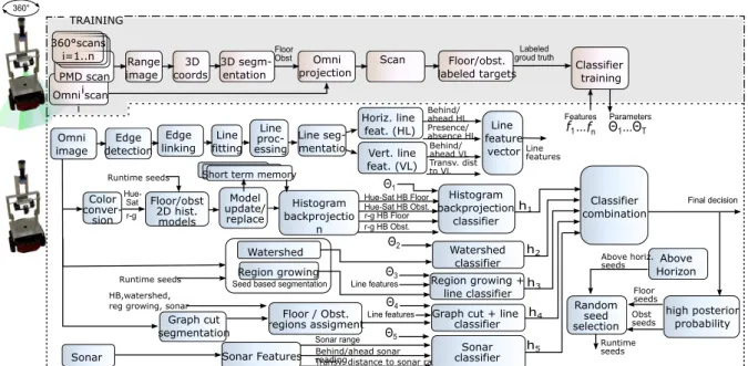
2.3.1 System Architecture
The overall system architecture is shown in Fig. 2.1. The upper part outlines the ground truth data generation for classifier training. The lower part depicts the fea- tures, segmentation schemes and the ensemble of classifiers. The ground truth labeled data (Fig. 2.2 is generated using a PMD camera that delivers 3D range data at a 204 x 204 pixel resolution across a 40 ◦ × 40 ◦ field of view. The PMD camera information only generates the ground truth for offline training and is not used at run time.
TRAINING
RUNTIME Omni scan
i
Floor Obst
Labeled groud truth Range
image 3D coords
3D segm- entation
Omni projection 360°scans
i=1..n Scan
PMD scan i 360°
Floor/obst.
labeled targets Classifier training
Color conver-
sion
Floor/obst 2D hist.
models
Model update/
replace
Histogram backprojectio
n
Hue-Sat HB Obst.
Hue- Sat
r-g
Hue-Sat HB Floor
r-g HB Obst.
r-g HB Floor
Watershed
Floor / Obst.
regions assigment
Sonar
Region growing
Graph cut segmentation
Sonar Features
Sonar range Seed based segmentation Runtime seeds
Runtime seeds
Θ
1...Θ
T ParametersHistogram backprojection
classifier Θ1
...
Features
f
1f
nWatershed classifier Θ2
Region growing + line classifier Edge
detection Edge linking
Line fitting
Line seg- mentatio
Horiz. line feat. (HL) Vert. line feat. (VL) Omni
image
Behind/
ahead HL Presence/
absence HL Behind/
ahead VL Transv. dist to VL
Line feature
vectorLinefeatures Line
proc- essing
HB,watershed, reg growing, sonar
Graph cut + line classifier
Random seed selection
high posterior probability Floor
seeds
Runtime seeds
Obst seeds
Above Horizon Above horiz.
seeds
Behind/ahead sonar reading
Classifier combination
Final decision
Transv. distance to sonar ray
h1
h2
h3 h4 h5 Short term memory
Θ3 Line features
Θ4
Sonar classifier Θ5
Line features
Figure 2.1: System architecture of the free-space detection with ensemble of experts
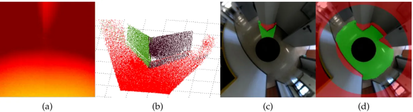
The depth image of different scenes, such as corridors, open rooms, and confined spaces, is obtained by rotating the robot and PMD camera by 360 ◦ and capturing scans at each pose. The 3D data from the PMD is subsequently fitted to planar surfaces us- ing random sampling consensus (RANSAC). Surface normal orientation, distance to the camera, and connected components determine whether a pixel and its associated 3D point are labeled as obstacles or floor.
The target floor-obstacle labels for each omni-image are generated after projecting the 3D labeled points into the omni-view. Furthermore, a complete 360 ◦ ground truth mask is generated by the superposition of overlapping scans (10 ◦ overlaps) from odometry and scan matching.
Fig. 2.2a-d illustrates the target data classification in the range image. Brightness
indicates proximity in the range image. The estimated planes in 3D space are each
marked with a different color in the point cloud. The 3D plane segmentations are
2.3 Free-Space Detection with Ensemble of Experts projected onto the corresponding sector in the omnidirectional view. The last step is the generation of the complete 360 ◦ ground truth mask employing scan matching.
At runtime, the sole robotic reactive behavior perceptions are the classification of the omnidirectional image into free space and obstacles.
(a) (b) (c) (d)
Figure 2.2: Ground truth data generation (a) Range image, (b) Planes fitted from the 3D data with RANSAC, (c) Projection into the omnidirectional view, (d) Ground truth data after 360 ◦ scan-matching and considering points over the horizon
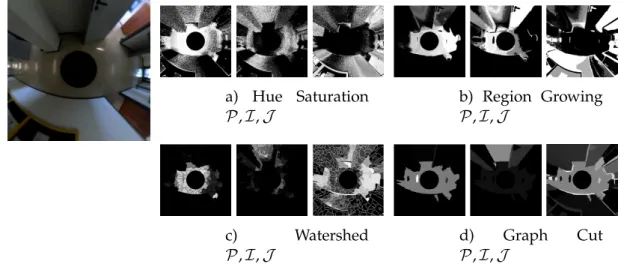
Four segmentation schemes generate heterogeneous segmentations: 2D histogram models; marker-based watershed and region growing that rely on seeds and the graph-based segmentation method an unsupervised approach. Further, the robot’s built-in sonar sensors provide depth information to the system with low angular resolution. Vertical and horizontal lines features that are strong obstacle indicators contribute further to enhance the region growing and graph-based segmentation by fusing their segmentation with geometric features. Only two segmentations are sup- ported with line features to obtain as heterogeneous as possible features and clas- sifiers. This diversity ensures that the classifiers make different errors at specific instances. This heterogeneity is a fundamental property of ensemble-based classifi- cation to reduce the generalization error compared to the individual classifier error rates.
Each classification expert constitutes a naive Bayes classifier that predicts the poste- rior probability of the class of a single-pixel as either floor or obstacle based upon the features and their likelihoods computed on the training set. The naive Bayes classifier, although it assumes conditional independence of features, achieves reasonable accu- rate classification at low computational complexity in comparison to more advanced schemes such as Bayesian networks. Notice that for reactive mobile robot navigation, a frame rate of 10Hz is desirable, thus requiring fast real-time image processing and classification.
For combining the expert evidence, we investigate four different combination meth-
ods [Pol06]: The stacked generalization approach, where the outputs of individual
classifiers serve as inputs to a second level meta-classifier; the behavior knowledge
space (BKS) that builds a lookup table that maps the possible combinations of mul-
tiple classifier decisions with the observed class frequencies in the training data and
finally two non-trainable aggregation rules based on the median and the majority
voting. Since the PMD data is not available at runtime, the seed-based segmenta-
tion algorithms obtain their seeds from pixels in the previous frame with high-class
2 Visual Range Sensor
confidence. Extracting seeds from the previous frame is reasonable, given that the optical flow between consecutive frames is low due to the wide field of view of the omni-camera and the high frame rate.
2.3.2 Segmentation and Features
Histogram Backprojection
Histogram Backprojection [SB91] identifies regions in the image which match with a reference model in appearance. The normalized histogram reference model M in a 2D color space is compared with the normalized histogram H of the current frame I and the backprojection image B is computed by
B ( u, v ) = min M ( c ( u, v ))
H ( c ( u, v )) , 1 , (2.3.1) in which c ( u, v ) denotes the 2D color of the pixel ( u, v ) . The backprojection image in the range between [ 0, 1 ] is interpreted as the degree of similarity between the region and the reference model.
Instead of merely generating a single color model of the floor, our approach main- tains additional models of the obstacles. Maintaining explicit appearance models of the obstacle regions refines the decision boundary between the floor and obstacles compared to a floor versus rest comparison. The omnidirectional view extends about 15 ◦ beyond the horizon line such that pixels above the horizon line certainly do not belong to the floor. Thus, the obstacle model is estimated from pixels above the cor- responding horizon circle in the omni-image. The 2D histograms are quantized into 32-32 bins to improve generalization, reduce the dimensionality, and are averaged and normalized A naive Bayes classifier based on histogram backprojection merges the information of the following four input features: The floor and obstacle model backprojection use the Hue-Saturation channel of the HSV color space; accordingly, the floor and obstacle model backprojection of the r-g channel of the RGB (normalized RGB space). Examples of the output of the histogram backprojection segmentation are shown in Fig. 2.3
(a) (b) (c) (d) (e)
Figure 2.3: (a) Input image (b) Hue-Saturation histogram backprojection with floor model (c) Hue-Saturation histogram backprojection with obstacle model (d) R-g histogram backprojec- tion with floor model (e) R-g histogram backprojection with obstacle model
Dynamic changes in slowly varying environments are addressed by updating the
histograms with an exponential moving average (EMA) whereas in rapid changes in
2.3 Free-Space Detection with Ensemble of Experts the scene, e.g., changes in the floor surface, a new model is instantiated rather than updating. This situation is identified with histogram-intersection, where a threshold value indicates no matches with the stored histograms. The maximum number of models stored simultaneously in short term memory is limited to five instances of obstacle models and two for the floor to meet computational demands. The EMA is computed with the following equation:
M ¯ ( x, y ) t = α M ( x, y ) t + ( 1 − α ) M ¯ ( x, y ) t − 1 (2.3.2) in which M t denotes the histogram of the current frame and ¯ M t − 1 the previous average. The smoothing factor α is set to 0.6 giving more importance to recent obser- vations. The histogram intersection is given by:
d ( M 1 , M 2 ) = ∑
x,y
min ( M 1 ( x, y ) , M 2 ( x, y )) (2.3.3) in which a score of one denotes an exact match and zero a complete mismatch.
In practice, a new model is initialized if the histogram intersection between the cur- rent frames and the most similar stored models falls below a threshold of 0.4. New histogram models replace the oldest model in case the maximum storage capacity is exceeded. Models that do not match with any of the thirty most recent frames are automatically discarded.
Marker-based Watershed
Marker-based watershed segmentation [RM01] is best understood by interpreting the gradient image as elevation information. The watershed lines coincide with strong image gradients. Pixels in the elevation image are attracted to their local minimum, thus forming so-called basins. Water is flooded evenly from each marker to flood the basins. The process stops once the water level reaches the highest peak in the landscape. Basins connected to the same original marker are merged into a single region. Fig.2.4 shows an example of watershed segmentation seeded with a random percentage of high confidence labeled seeds.
(a) (b) (c)
Figure 2.4: Watershed segmentation: (a) Input image (b) Marker-based watershed with ran-
dom seeds (c) Resulting watershed segmentation knowing the floor/obstacle seeds selected at
points with high posterior probability
2 Visual Range Sensor
Graph-based Segmentation
Graph-based segmentation is described in [FH04]. This method is highly efficient and produces segmentations based on a region comparison function that considers the minimum weight edge in a graph between two regions in measuring the differ- ence between them. The graph is constructed in such a way that image pixels are transformed into a feature space vector that combines the ( x, y ) pixel location with its RGB color value. Edges in the graph connect points that are close in the feature space. The assignment of whether or not a region belongs to the ground or obstacles, is determined with information from previous segmentations.
Given the unsupervised nature of this algorithm, it is common to find situations where the segmentation grows unbounded. It is, therefore worthwhile to fuse the graph-based segmentation in the classifier with the line features. Fig. 2.5 illustrates the graph-based segmentation, the floor-obstacle assignment and the benefit of using line features to prevent unbounded region growing.
(a) (b) (c) (d)
Figure 2.5: Graph-based segmentation: (a) Input image (b) Graph-based segmentation (c) Floor-obstacle assignment to the graph-based regions from the previous segmentations; d) Output of the classifier after merging the line features
Region Growing
Region growing starts with a set of seed points, and neighboring pixels are added based on their similarity in an incremental fashion to a region. Each segmentation originates from a single seed of known class labels. Region growing segmentation is repeated N i times with different seeds randomly sampled from pixels classified in the previous image with high confidence. After N i random region growing repetitions, N i ( u, v ) counts how often the pixel ( u, v ) is part of the final region, thus indicating the similarity of that pixel with prototype pixels of class λ i . It is important to notice that a pixel that is not captured by a particular region growing instantiation might still belong to the corresponding class, as region growing is a local method and only expands to those pixels that are connected with the original seed. In particular, the obstacle regions are often fragmented due to the multitude of objects. Therefore, it is essential to relate the absolute counts to the average number of pixels < M ki > in a single region growing segmentation. A pixel has a membership degree to class λ i
given by
µ i ( u, v ) = max { N i ( u, v ) N i
∩ M i
M i , 1 } . (2.3.4)
2.3 Free-Space Detection with Ensemble of Experts The relative frequency N i ( u, v ) /N i is scaled by the ratio between the size of the union of all segmentations ∩ M i of class λ i and the average size M i of a single segmented region. The ratio is a coarse estimate of the number of fragmented segments of a class.
Therefore, the score of a fragmented class is weighted more strongly in comparison to a class that forms a connected region.
(a) (b) (c)
Figure 2.6: Region growing segmentation: (a)Input image (b) Region growing (c) Classifier output of region growing plus line features
Inverse Sonar Model
The sonar classifier computes the posterior probability of a pixel belonging to a class floor, obstacle based on the observed likelihoods p ( C i | r, d, a ) . The feature r corre- sponds to the discretized sonar range reading and is limited to ten discrete values. d is the lateral distance of a pixel to the nearest sonar ray projected into the omni image, and a denotes whether a pixel in the radial direction is in front or behind the nearest sonar range reading. An example of the sonar classifier output is shown in Fig. 2.7.
Notice that sonar range readings might be misleading, such as the two range readings in the north-west direction that overestimate the extension of free space.
(a) (b)
Figure 2.7: Sonar classifier: (a) Input image, with projected sonar readings (b) Output of the sonar classifier
Segmentation Based on Lines
Edges often correspond to image regions at which the scene exhibits discontinuities in
shape, depth, or variation in material properties. In our context, they suffer from the
disadvantage of high sensitivity to variations in the scene illumination. Nevertheless,
2 Visual Range Sensor
(a) (b) (c) (d)
Figure 2.8: Line features: (a) Input image (b) Canny edge detection (c) Edge linking and line fitting (d) Vertical/horizontal lines
edges are strong indicators of the presence of obstacles and provide a valuable cue to enhance the classification of region growing and the graph-based segmentation.
Rather than using merely the edge information at a pixel level, their connectiv- ity is considered. Edges are linked by contour following and subsequently fitted to lines using a split approach. Contours are first globally approximated by a straight line connecting the endpoints. Consequently, they are recursively split at the points of maximum traversal deviation. The resulting lines are classified into vertical and horizontal lines according to their orientation in the omniview. Lines not belonging to either orientation or lines that are too short are discarded. Vertical lines appear radially distributed in the omni-image and in general correspond to typical indoor environment objects such as shelves, cabinets, cupboards or table legs. A horizontal line may indicate the presence of obstacles such as walls, doors or tables.
Four line features are defined accordingly: a) ahead or below a horizontal line;
b) Presence or absence of horizontal lines; this is determined for each pixel u, v by verifying if there is an intersection of a horizontal line with the projected line formed by the pixel u, v and the image center; c) ahead or below a vertical line; d) transversal distance to the closest vertical line.
Naive Bayes Classification
The ensemble of experts is constituted by five Naive Bayes classifiers as shown in Fig. 2.1. The likelihood p ( x i | C j ) of a feature x i given the class C j is modeled by a Gaussian distribution in the case of continuous features, and by a multinomial distri- bution in the case of discrete features. The likelihoods of the data and the class priors are estimated from the observed frequencies of classes and features in the training data. The naive Bayes classifier computes the a posteriori probability of the classes C = { Floor, Obstacle } according to the likelihood of the conditionally independent features:
p ( C j | x ) = 1 Z
∏ n i = 1
p ( x i | C j ) p ( C j ) (2.3.5)
in which the normalization factor Z is the evidence of the features x. The ulti-
mate decision boundary is determined by the problem-specific relative costs of false
positive and false negative classifications.
2.3 Free-Space Detection with Ensemble of Experts
2.3.3 Experimental Results
The training data consists of almost two million pixels captured from 500 images of which the true class label is established from the PMD depth information and 3D segmentation. The classification performance is validated on 500 additional un- seen images with ground truth obtained from PMD data. The training in the case of stacked generalization follows a k-fold selection in which the training data set is divided into T blocks, in which T denotes the number of classifiers participating in the ensemble. Each single classifier is trained with T − 1 blocks of data; thereby, each classifier does not see one block of data. The outputs of the classifiers on the unseen block, in conjunction with the ground truth segmentation, constitute the training pairs for the second level meta-classifier. Once the second level classifier is trained, the T classifiers are retrained with the entire training data set. The segmentation accu- racy is determined based on the false positive rate FPR, the number of false positives divided by the total number of negatives; and true positive rate TPR, the number of true positives divided by the total number of positives. A false negative is constituted by a floor pixel incorrectly classified as an obstacle, and a false positive is an obstacle pixel incorrectly labeled as floor.
Table 2.1: Classifiers performance
Method FPR TPR
Histogram backprojection 0.085 0.889
Watershed 0.042 0.945
Watershed + line features 0.036 0.938
Region growing 0.120 0.718
Region growing + line features 0.044 0.907
Graph segmentation 0.064 0.869
Graph segmentation + line features 0.023 0.917
Sonar 0.045 0.890
Combination with stacked generalization 0.032 0.958
Combination with BKS 0.030 0.912
Combination with median 0.024 0.945
Combination with majority voting 0.024 0.927
Table 2.1 compares the true positive and false negative rates of the output of every
single classifier, namely histogram backprojection, watershed, region growing, graph
segmentation and sonar. The fusion of vertical and horizontal lines features in re-
gion growing and graph segmentation clearly improves the performance of these two
classifiers. Using line cues in conjunction with watershed does not improve its ac-
curacy, as watershed itself is already based on edge features. Notice, that watershed
and graph cut in isolation are unsupervised segmentation schemes not suitable for
classification. They instead inherit the classification from the proper labeling of seeds,
which in this case, are provided by stacked generalization. Therefore, their reported
accuracy in Table 2.1 has to be attributed to the ensemble of classifiers rather than the
watershed and graph-based segmentation itself.
2 Visual Range Sensor
Stacked generalization exhibits the best classification rate in terms of FPR among all classifier ensemble methods. The inferior performance of BKS combination is at- tributed to the binarization of the posterior probabilities for the generation of the lookup table that results in loss of information that is available to stacked gener- alization. Even though median and majority voting combination rules require no second-level training, they demonstrate the best performance in terms of FPR. In the context of obstacle avoidance, false-positive classification is more critical since missing an obstacle is potentially more severe than underestimation of the free space. One of the main properties of the median combination is to filter out segmentations that are outliers.
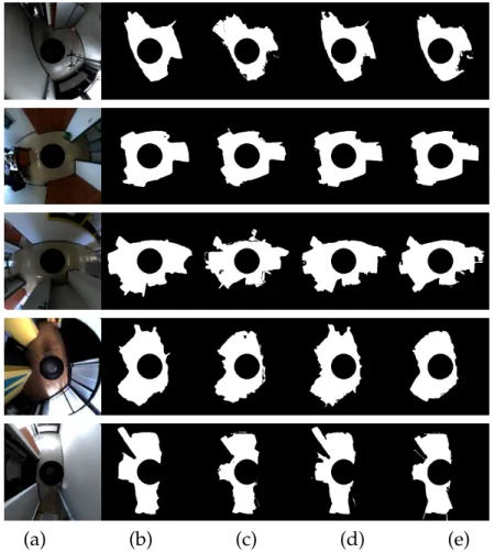
Fig. 2.9 shows the results of four prototypical scenarios, with the corresponding output of the four combination methods. The first scene exhibits misleading specu- lar reflections and shadows that are incorrectly segmented based on color information alone. The vertical line features increase the segmentation performance since the three vertical posts in the bottom right part of the image are correctly segmented from the floor, even though some of the first level classifiers ignore them. The second sce- nario illustrates a typical office environment with a rather high contrast between floor and obstacles. The specular reflections on the surface are still correctly classified as floor. The third to fifth scenarios illustrate segmentation tasks that exhibit substantial variations in illumination, reflections, and shadows.
(a) (b) (c) (d) (e)
Figure 2.9: Segmentation examples: (a) Input image, (b) Stacked Generalization, (c) Behavior
Knowledge Space, (d) Median combining rule, (e) Majority voting.
2.4 Online Self-Supervised Free-Space with Range Image Data
2.4 Online Self-Supervised Free-Space with Range Image Data
In the previous section, we discussed a segmentation approach based on supervised learning from offline data by fusing with a mixture of experts different heterogeneous segmentations and features. In this section, we explore a self-supervision method [Pos+10b] by online combining 3D information of the Range image to gather more insight into the visual data in the omnidirectional image.
The approach employs a 3D camera to obtain ground truth segmentations in a narrow frontal field of view. The accuracy of alternative segmentation schemes in conjunction with alternative visual cues is evaluated by cross-validation over 3D scans on the frontal view. The combination that performs best in the current context is then applied to segment the omnidirectional view providing 360 ◦ depth information.
The range data in the front view provides the seeds and validation data to super- vise the appearance-based segmentation in the omniview. The Segmentation relies on histogram backprojection, which maintains separate appearance models for floor, obstacles, and background.
2.4.1 System Architecture
The camera system consisting of a PMD and an Omnidirectional camera is mounted on the Pioneer 3DX mobile robot, as shown in Fig. 2.10. The 40 ◦ x 40 ◦ field of view of the time-of-flight (ToF) camera and the 75 ◦ vertical of the omnidirectional are directed towards the floor and both camera’s fields of view intersect in a narrow region in front of the robot.
1 3m
° 5
4 0 ° 40 ° 60 °
>10m
ToF Camera FOV Omnidirectional
Camera FOV
Figure 2.10: Configuration and field of view of the PMD camera and the omnidirectional camera
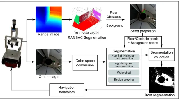
The overall system architecture is shown in Fig. 2.11. The online segmentation pro-
ceeds in four stages: a) range image segmentation into planar regions; b) projection of
2 Visual Range Sensor
these regions into the omnidirectional view; c) omniview segmentation; d) validation and selection of optimal segmentation and cue.
Figure 2.11: System architecture of the online self-supervised free-space detector
2.4.2 Validation Data with a Range Camera
The validation data is generated similar to the technique used in the previous section to obtain the 360 ◦ training mask. A 3D scan of the frontal region is segmented into planar surfaces using RANSAC. These segments are then classified according to the orientation of the surface normal, distance to the camera and area into three cate- gories: ground considered as free space, vertical planes and obstacles. Scan points that do not belong to a surface are ignored. These labeled regions are projected as ground truth segmentation into the omnidirectional view. This ground truth allows the selection of the visual cue and segmentation method that is optimal for the ap- pearance and illumination of the local environment. Part of the 3D scan segmentation is utilized as seeds for the subsequent 2D appearance-based segmentation; the re- maining data is used to validate the performance of alternative segmentations and cues.
RANSAC is applied iteratively, such that the scan points that belong to the plane with the most inliers are removed from the data set. The next plane is estimated from the residual points until the number of points belonging to the best surface model falls below a threshold. The classified 3D points are projected into the omnidirectional view as shown in Fig. 2.12. It illustrates the range image in which brightness indicates proximity, the estimated and labeled planes in 3D space, and the projection of these labels onto the corresponding sector in the omnidirectional view.
A key aspect of marker or seed-based segmentation algorithms is the selection of
initial seeds. The more informative the set of seeds, the better the final segmenta-
tion result. Similar to the previous Section, in the online segmentation, we employ
four alternatives: segmentation based on color histogram backprojection in two dif-
ferent color spaces (hue-saturation and normalized red-gree), watershed algorithm,
2.4 Online Self-Supervised Free-Space with Range Image Data
(a) (b) (c)
Figure 2.12: Seeds projection: (a) Range image, (b) Planes fitted from the 3D data with RANSAC, (c) Seeds projected into the omnidirectional view.
and model-based region growing. Although we acknowledge the potential utility of other appearance features such as texture [Bla+08], only color is considered as it is difficult to extract reliable texture due to the low resolution of the omni-image.
No single segmentation scheme alone provides a robust, accurate segmentation across all scenes. The idea is, therefore, to validate the accuracy of segmentation on labeled ground truth data and then to select the method best suited for the current floor texture and illumination. For this purpose, the ground truth segmentation data obtained from the 3D scans is partitioned into training and validation data (Fig 2.13).
The training data is used to build the reference model for the histogram backprojec- tion and to provide the initial seeds for marker-based watershed and region growing.
Training Validation
Floor training Obstacle training
Floor correct segmented Obstacle correct segmented False positive False negative Outside FOV
Figure 2.13: Segmentation validation
False positive rate and false negative rate are aggregated into a total classification error
f = ( 2 f p + f n ) /3 (2.4.1)
in which false positives are weighted twice as strong since an obstacle miss is poten- tially more severe in the context of obstacle avoidance.
The segmentation validation utilizes two-fold cross-validation, in which the roles of
the training dataset and the validation dataset are reversed and the classification error
is averaged over both folds. The segmentation method with the lowest aggregated
2 Visual Range Sensor
classification error is applied to the entire omnidirectional view. In order to save computational resources, the segmentation validation and selection is only repeated every fifth frame. The final segmentation is filtered by a 5x5 median filter in order to eliminate isolated pixels and noise.
2.4.3 Experimental Results
The performance of the system is validated on 500 images with ground truth ob- tained from PMD data and 30 images in which the actual floor area is segmented by hand. Table 2.2 compares the true positive and false negative rates of watershed and region growing seeded with one percent of labeled pixels as seeds, and histogram backprojection using different models according to the seeds: floor, obstacles, and background. From the results, we can conclude that selecting among several alter- native models outperforms using a single floor model. Hue and saturation are more reliable cues compared to normalized color ( r and g). On both test sets, the hue saturation classifier with three models achieves true positive (floor classified as floor) rates between 0.85 − 0.9 if one accepts a false positive (obstacle classified as floor) rate between 0.1 − 0.13. Selecting the best among all segmentation leads to the value of 0.085 (lowest false positive rate in the hand-labeled set) In the context of navigation, the false positive rate is the critical variable to consider since missing an obstacle is more severe than underestimating the free space.
The classification performance is similar across the PMD validation, and the hand- labeled data set. In fact, the classification error on the hand-labeled data is even lower. We attribute this phenomenon to the fact that the depth-based segmentation is less accurate than hand segmentation. Thus, the test data set itself contains a small fraction of incorrect samples that contribute to the classification error.
The classification performance of watershed and region growing is superior on the PMD test set, with watershed outperforming region growing. It is not surprising that watershed and region growing achieve high classification rates on the PMD test set, as the seeds stem from the same narrow frontal region as the test data. The true generalized classification error of watershed and region growing becomes apparent on the manually labeled data set, in which the test data is uniformly distributed across the omnidirectional view. The dependence of watershed and region growing on a representative set of seeds is a definite disadvantage over more robust histogram backprojection.
Figure 2.14 shows the results of eight prototypical scenarios, together with the cor-
responding floor segmentation results. The system is robust even with a tiled floor,
strong sun reflections, and imperfect lighting conditions. The second-row example
shows the ability to adapt to new unseen floor surfaces where floor color and texture
abruptly change behind the door.
2.4 Online Self-Supervised Free-Space with Range Image Data Table 2.2: Comparison of the segmentation schemes under two data sets
PMD ground truth Hand labeled
Method FPR TPR FPR TPR
H-S histogram features: F 0.173 0.855 0.089 0.905 H-S histogram features: F | O | 0.123 0.845 0.094 0.971 H-S histogram features: F | O | B 0.137 0.845 0.096 0.911 r-g Histogram features: F 0.210 0.828 0.118 0.923 r-g Histogram features: F | O 0.145 0.836 0.105 0.870 r-g Histogram features: F | O | B 0.147 0.825 0.112 0.896
Watershed 0.021 0.948 0.140 0.749
Region growing 0.097 0.932 0.149 0.676
Histogram all Feat. + Watershed + Region Growing
0.158 0.867 0.085 0.904
F: Floor, O: Obstacle, B: Background