A Field Theory Approach to Universality in Quantum Chaos

(1)

A Field Theory Approach to Universality in Quantum Chaos

Inauguraldissertation

zur Erlangung des Doktorgrades der

Mathematisch–Naturwissenschaftlichen Fakult¨ at der Universit¨ at zu K¨ oln

vorgelegt von

Jan M¨ uller

aus K¨ oln

K¨ oln 2007

(2)

Tag der m¨ undlichen Pr¨ ufung: 12. Januar 2007

(3)

Abstract

We show that in f ≤ 3 dimensions, the spectral statistical properties of a certain en- semble of quantum mechanical systems, chosen such that these systems share the same classical limit, are universal provided that the underlying classical dynamics is chaotic.

These universal properties are faithful to random matrix theory up to universal correc- tions due to quantum interference effects, which stem from the Heisenberg uncertainty relation. In addition, we explain the formation of a universal gap in the electronic spec- trum of a normal conducting chaotic system when the latter is brought in contact with a superconductor. This gap opens in the vicinity of the Fermi surface and its universal width is also set by quantum uncertainty. The method which we employ is the ballistic σ–model, a quantum field theory which is known for ten years now but whose evaluation was to date only possible with additional assumptions which we identify to be dispens- able upon closer inspection. The insights gained enable us to draw novel parallels to the semiclassical approach and to the theory of dynamical systems.

Zusammenfassung

Wir zeigen, daß in f ≤ 3 Dimensionen die Spektralstatistik eines gewissen Ensembles quantenmechanischer Systeme, die den gleichen klassischen Limes haben, universell ist, sofern die zugrundeliegende klassische Dynamik chaotisch ist. Insbesondere deckt sich dieses universelle Verhalten mit dem von Zufallsmatrixensembles bis auf universelle Kor- rekturen, die durch Quanteninterfenzeffekte entstehen und auf die Heisenbergsche Un- sch¨ arferelation zur¨ uckzuf¨ uhren sind. Dar¨ uberhinaus erkl¨ aren wir die Entstehung einer uni- versellen L¨ ucke im elektronischen Spektrum eines normalleitenden chaotischen Systems, sobald dieses in Kontakt mit einem Supraleiter gebracht wird. Diese L¨ ucke entsteht in der N¨ ahe der Fermikante, und ihre universelle Breite wird ebenfalls durch Quantenunsch¨ arfe gesetzt. Als Methode verwenden wir das ballistische σ–Modell, eine Quantenfeldtheorie, die seit zehn Jahren bekannt ist, deren Auswertung bisher aber nur mithilfe zus¨ atzlicher Annahmen m¨ oglich war, die wir durch eine sorgf¨ altigere Betrachtung als entbehrlich herausstellen. Durch die gewonnenen Erkenntnisse sind wir in der Lage, neue Parallelen zum semiklassischen Ansatz und zur Theorie dynamischer Systeme zu ziehen.

3

(4)

(5)

Chapter 1 Quantum chaos and universality

This chapter provides the background needed to place this thesis into context. The first section 1.1 is dedicated to explaining the term ‘quantum chaos’ and some of its most prominent universal features. The subsequent two sections serve as introductions to later chapters: while section 1.2 briefly sets the historical stage for the physics of the proximity effect to be discussed in chapter 3, section 1.3 reviews the basics of the semiclassical approach to quantum chaos. The latter section is a bit more detailed than the other introductory sections as it serves as a primer for chapter 5, where we are going to elaborate on the parallels between the semiclassical approach and the field theoretical formalism presented in this thesis.

1.1 Introduction

In the last century, it has become clear that there are two radically different types of classical Hamiltonian motion: regular and chaotic dynamics.

¹

Perhaps the most easily accessible difference between these two classes is the sensitivity to deviations of the initial conditions. While the final deviation of two originally close–by states only grows linearly in time in a regular system, the same error grows exponentially in chaotic systems.

Accordingly, regular systems are analytically under control. In fact, the semiclassical approximation is perfectly understood and exact for regular systems, and it is the Bohr–

Sommerfeld quantization scheme which led to an extrapolation of the quantum laws from the macroscopic world. The high degree of symmetry which stems from the independent integrals of motion manifests itself in the quantum spectrum through the independence of disjoint spectral series. In fact, at sufficiently large energies, the eigenvalues of a regular quantum system are completely randomized and appear to be Poisson distributed over the energy axis. Of course, the complexity of chaotic motion leaves one helpless in the first place. How would one establish a semiclassical correspondence? There is no such vehicle as the action–angle variable pairs which allows a neat classification of orbits. Quite on the contrary, the chaotic dynamics will eventually bring each orbit close to any other orbit, and these ‘spaghetti’ of trajectories are rather perplexing. One might then think that one just has to accept that there is no remedy but to merely take the quantum laws which one has guessed successfully from the classical world and to quantize the chaotic

1

For a more profound introduction to the topics covered here we refer to the textbooks [1, 2, 3].

7

(8)

Hamiltonian at hand. No need for a semiclassical correspondence in the ‘generic’ case beyond this.

Interestingly, however, it turns out that the qualitative difference of chaotic dynamics leaves characteristic footprints in the quantum world: these quantum signatures of chaos are commonly termed ‘quantum chaos’. Let us start our journey in the late 1950s/early 1960s, when Wigner and Dyson successfully applied statistical methods in order to de- scribe the spectra of heavy nuclei, systems beyond the reach of standard quantum mech- anical methods [4, 5, 6]. These latter methods are known to always rely on some high degree of symmetry and can at most deal with small perturbations of some primitive reference system such as a harmonic oscillator, a hydrogen atom, or some free particle or spin. However, by the experience from statistical mechanics, the complexity of chaotic dynamics represents a promising weak spot. Inspired by that observation, Wigner and Dyson modeled nuclei by statistical ensembles of random Hamiltonian matrices which respect the basic symmetries such as rotational or time reversal symmetry and are oth- erwise maximally entropic. This so–called random matrix theory (RMT) allows a very accurate prediction of the statistical spectral properties of sufficiently complex quantum systems. The characteristic feature of the resulting quantum spectra is a high degree of regularity : the eigenlevels tend to repel each other and to arrange themselves on a one–dimensional lattice with fluctuations about the equilibrium value which are universal in the sense that (upon proper rescaling of energies in units of the local mean level spacing) they only depend on the underlying symmetries of the given system.

While anyone who has had some exposition to standard statistical mechanics might say now that this universality is not very surprising at all, it is indeed very striking inas- much as there is no proper explanation as to how this universality arises in an individual system. Quantum mechanics is a linear theory and therefore apparently ignorant of the non–linear complexity which is characteristic for classical chaos. It took twenty years to distill the criterion which is responsible for universality. Based upon empiric results, Bohigas, Giannoni, and Schmit (BGS) formulated a conjecture in 1984 [7]:

• If the underlying classical dynamics of a quantum system displays ‘generic’ chaos, then the statistical spectral properties of that system are universal and depend only on the symmetries of that system.

This celebrated conjecture is infamous inasmuch as it has kept a whole industry of

‘quantum chaologists’ busy ever since.

²

The 1980s and early 1990s brought a wealth of experimental results which substantiated the BGS conjecture and illustrated how deviations from RMT may arise [8, 9, 10]. Universal spectral statistics of the RMT type has been observed in totally different systems ranging from the energy levels of heavy nuclei, highly excited (so–called Rydberg) atoms, and mesoscopic structures such as two–dimensional electron gases, up to microwave modes in quasi two–dimensional cavities and ordinary sound modes in rigid bodies. RMT statistics even serves as a null model for the eigenvalues of stock–market price covariance matrices and helps to identify non–trivial correlations, say, among different industry sectors. As a more abstract phenomenon, also the zeroes of the Riemann zeta function display RMT statistics, and the mathematicians hope to find a physical system (the ‘Riemannium’) whose spectrum coincides with these zeros. In contrast to this, positive theoretical progress towards a

2

For a review and a wealth of references cf. the monographies by St¨ ockmann [1] and Haake [2].

(9)

1.1 Introduction 9

proof of the BGS conjecture went rather stagnant. As a first line of research, there is the semiclassical approach which employs the Gutzwiller trace formula in order to express spectral properties in terms of classical dynamical quantities. The semiclassical branch will be reviewed in some detail in subsection 1.3. As an orientation as to how slow progress went, the milestones date to 1985 (Berry [11]), 1996 (Bogomolny &

Keating [12]), and 2001 (Sieber & Richter [13]). The work by Sieber & Richter (SR) took quantum uncertainty

³

into account and ignited a wave of publications [18, 19, 20, 21, 22, 23, 24, 25] which culminated in a fairly complete semiclassical understanding of spectral correlations.

An alternative approach dates back to 1983, a time even prior to the BGS conjecture, when Efetov employed field theoretical methods to prove that the statistical spectral properties of disordered systems are faithful to RMT [26]. Efetov’s theory was formulated in terms of the so–called diffusive non–linear σ–model. The name alludes to the fact that a perturbative evaluation of this model is formulated in terms of a diffusion–type propagator (Dq

²

− iω/ ~ )

⁻¹

. In a system of finite extension L, this propagator displays a gap of the order of the Thouless energy E

_c

≡ ~ D/L

²

; that is, for energies below this threshold only the homogeneous (q = 0) configuration remains dominant while inhomogeneous configurations become strongly suppressed. The effective low–energy theory is thus governed by the so–called ‘zero–dimensional’ σ–model, which is just jargon for a reduced field space which is structureless in configuration space. Efetov employed the supersymmetric formulation of the zero–dimensional σ–model and showed how to derive the RMT answer from it. While this seminal result is not directly applicable to the realm of clean chaotic systems, it illustrates how powerful field theoretical methods are in deriving universal properties.

Tempted by that promise and as late as 1995, Muzykantskii & Khmel’nitskii formu- lated the counterpart of the diffusive σ–model for clean systems [27]. In field theory jargon, clean is synonymous to ‘ballistic’,

⁴

and consequently the resulting field theory was termed the ballistic σ–model. This model is the central object of interest to this thesis. It is formulated in terms of fields which reside on classical phase space, and its perturbative evaluation is formulated in terms of the Liouville propagator of phase space densities. The ballistic σ–model therefore promises to even allow a systematic study of non–universal properties of clean systems. Perhaps yet more attractive is that a reduction of its field space to those configurations which are homogeneous on phase space again yields the zero–dimensional σ–model and hence the RMT answer. That this expectation once might prove successful is backed up by the fact that the Liouville propagator of chaotic systems is highly unstable against noise. Namely, in the presence of noise, the Liouville propagator acts on a reduced space of smooth phase space densities.

The resulting object is called the Perron–Frobenius propagator and is known to display a gap ~ /t

_mix

against the homogeneous configuration, just like its diffusive cousin.

⁵

Inter-

3

Quantum uncertainty is reflected in a finite so–called Ehrenfest time, the time it takes to amplify quantum details to classical size by means of Lyapunov expansion. This time scale was first identified by Larkin & Ovchinnikov in the 1960s [14, 15]. It was again (Aleiner and) Larkin [16, 17] who in 1996 first identified the Ehrenfest time to play a pivotal role in quantum chaos.

4

This terminology alludes to the ballistic (diffusive) motion of electrons in a clean (disordered) system.

5

In fact and as a crucial point of this thesis, the propagator of the ballistic σ–model turns out to be

indeed the Perron–Frobenius propagator, but may not be evaluated in the na¨ıve sense that it becomes

(10)

estingly, taking the long–time limit first, this gap even prevails in the limit of vanishing noise. This is one of the rare (but usually fundamental) cases in physics where two limits

— in the case at hand the long–time limit and the limit of vanishing noise — do not commute. Altogether this field theory was very appealing to condensed matter physicists and promised them a way to explain how universality emerges in quantum chaos.

So it took only another year until Andreev et al. proposed a derivation of the ballistic σ–model in their seminal works [28, 29]. Building upon the observation that it always takes some statistical ensemble to average over in order to derive an effective field theory, they took advantage of the fact that spectral correlations are invariant under translations of the spectrum. Averaging over this reference energy, Andreev et al. were able to derive the action by Muzykantskii & Khmel’nitskii from first principles. In the following years and even in the original works, however, a number of drawbacks were identified which plagued both the derivation and the evaluation of the effective theory [28, 29, 30, 31, 32].

Apart from the phenomenological (nevertheless very insightful) works by Larkin and collaborators [16, 17, 33, 34] and Altland & Taras–Semchuk [35] on the topic of quantum interference effects, it is safe to say that the drawbacks of the ballistic σ–model have remained unresolved to date. This thesis aims to reconsider these problems in depth and to cure most of them.

But before, let us provide some more background on universality in quantum chaos in the remainder of this introductory chapter. First, we are going to give a brief account of the history of the ‘proximity effect’, a term for the anomalous properties which nor- malconducting systems inherit from an adjacent superconductor. After that we aim to review the basic ideas entering the semiclassical approach to universal spectral correla- tions. These ideas rely on the phenomenon of quantum interference, hence the title of that section. We conclude with an outline of this thesis.

1.2 The proximity effect

It was as early as in the 1960s [36] that superconductors were found to tend to export some of their anomalous properties to adjacent normal conducting materials.

⁶

This so–called ‘proximity effect’ has been of great interest to mesoscopic physics ever since.

Perhaps the most direct manifestation is the suppression of the density of states (DoS) in the vicinity of the Fermi surface. More importantly to us, depending on the nature of the underlying classical dynamics of the normal region, this suppression falls into one of only two qualitatively different categories [41, 42]: while the suppression is approximately linear in the integrable case, the DoS displays a finite ‘Andreev’ gap otherwise. This result has been experimentally tested on normalconducting films on superconducting substrates [43]. While no gap was observed in the clean case, a gap opened in the presence of disorder. Yet, for clean systems which are non–integrable merely due to their chaotic classical dynamics, the formation of a gap is to date but an expectation backed up

homogeneous for times scales in excess of t

mix

. It is more adequate to think of it as a discretized version of the Liouville propagator, where the discretization length scales (due to quantum uncertainty) as ~ ; this object is protected against decay to universality up to the Ehrenfest time (cf. the discussion in section 1.3 and chapter 4), and only after this delay time has elapsed, it decays on the time scale set by t

_mix

.

6

For extensive reviews cf. [37, 38, 39, 40].

(11)

1.3 Quantum interference: Semiclassical background 11

by numerical results while an experimental verification is still lacking (cf. the review [40]).

Due to technological progress experiments might nevertheless soon come into reach. For example it is possible to fabricate billiards of almost ballistic two–dimensional electron gases which are coupled to a superconductor (cf. [44] and references therein).

We already have encountered a spectral ‘litmus test’ for classical chaos in the in- troduction, namely the formation of non–trivial and universal spectral correlations. In contrast to the latter, the proximity effect is based on the DoS itself. Similar to the BGS conjecture, the Andreev gap turned out to be recalcitrant to theoretical explanation. An important step was taken by Lodder & Nazarov (LN), who built upon the Eilenberger equation to relate the DoS to the distribution of lengths of classical paths in the normal region [45]. They found that since paths of any length (and thus of arbitrarily long flight time) exist there are states down to even the lowest energies. In other words, they could not confirm the formation of a gap in the DoS. This is not what one expects since quantum uncertainty sets a minimal resolution in phase space below which the notion of individual trajectories loses its meaning. Indeed, in chaotic systems, the quantum uncertainty is amplified to classical dimensions after the so–called Ehrenfest time t

_E

, so trajectories longer than t

_E

should have established contact to the superconductor and not contribute to the DoS any more. Correspondingly, LN themselves already conjec- tured the presence of a gap of the order of ~ /t

_E

.

⁷

This conjecture was substantiated phenomenologically by Taras–Semchuk & Altland [35] and Vavilov & Larkin [33] and has been tested numerically [41, 42]. Nonetheless, the question remains how quantum uncertainty enters the ‘hard–core’ quasiclassics ` a la LN. Building upon the basic field theoretical framework developed in chapter 2, we will turn to this question in chapter 3.

1.3 Quantum interference: Semiclassical background

In this section we review the semiclassical results for the behavior of globally hyper- bolic (chaotic

¹

) quantum systems at time scales t larger than the mixing time t

_mix

yet smaller than the Heisenberg time t

_H

≡ 2π ~ /∆. While the first condition implies that non–universal aspects of the classical dynamics are inessential, the second ensures that concepts of perturbation theory (in the parameter τ ≡ t/t

_H

) are applicable. If not men- tioned explicitly otherwise, the results covered here are a strongly simplified condensate of recent publications by the Haake group [22, 23].

To describe correlations in the spectrum of the system we consider the two–point correlation function

R

₂

(ω) ≡ ∆

²

ρ(E + ω/2)ρ(E − ω/2)

E

− 1 (1.1a)

and its Fourier transform

K(t) ≡ 1

∆ Z

dω e

⁻^~ⁱ^ωt

R

2

(ω), (1.1b)

7

If the Ehrenfest time is finite, the gap is ∼ min{ ~ /t

_D

, ~ /t

_E

}, where t

_D

is the dwell time of the normalconducting region [40].

1

In fact, all results apply to general mixing rather than just uniformly hyperbolic systems. The point

is that mixing implies ergodicity and non–integrability, and hence any mixing system will appear to have

constant global Lyapunov exponents when evaluated on time scales t t

_mix

.

(12)

the spectral form factor. Here, ρ(E) is the energy dependent DoS, and

· · ·

E

denotes the average over a sufficiently large portion of the spectrum centered around some refer- ence energy E

0

. In semiclassics, one makes use of the representation of the (oscillatory part of the) DoS by means of the Gutzwiller trace formula [46, 47]

ρ(E) − ρ(E)

E

∼ 1 π ~

Re X

γ

A

_γ

e

^iS^γ^/^~

(1.2)

to express the spectral form factor as K

_sc

(τ) = DX

γγ⁰

A

_γ

A

^∗_γ0

e

^i(S^γ^−S^γ⁰^)/^~

δ

τ − T

_γ

+ T

_γ⁰

2t

_H

E

, (1.3)

where the sums are over periodic orbits γ and γ

⁰

, S

_γ

the classical action of the orbit γ, T

γ

its revolution time, and A

γ

its classical stability amplitude.

Before turning to a more detailed discussion let us briefly summarize the main results recently obtained for the semiclassical form factor: for times τ < 1, K

_sc

can be expanded in a series in τ. As shown by Berry [11], the dominant contribution to this expansion, K

sc⁽¹⁾

= 2τ , is provided by pairs of identical (γ = γ

⁰

) or mutually time reversed (γ = T γ

⁰

) paths.

⁸

All corrections to the leading contribution K

sc⁽¹⁾

hinge on the mechanism of quantum interference. E.g., the sub–dominant contribution K

sc⁽²⁾

to the form factor is provided by pairs (γ, γ

⁰

) that are nearly identical except for one ‘encounter region’:

in this region, one of the paths self–intersects

⁹

while its partner just so avoids the intersection (cf. figure 1.1). Alternatively, one may think of two trajectories that start out nearly identical, then split up and later recombine to form an interfering Feynman amplitude pair. The two paths are, thus, topologically distinct yet may carry almost identical classical actions [16]. Specifically, SR [13] have shown that for sufficiently shallow self intersections (crossing angle in configuration space of O( ~ )) the action difference |S

_γ

− S

_γ⁰

| . ~ . For these angles, the duration of the encounter process is of the order of the Ehrenfest time

t

_E

≡ 1 λ ln c

²

~

(1.4) where λ is the phase space average of the dominant Lyapunov exponent of the system and c a classical reference scale (see below) whose detailed value is of secondary importance.

This identifies t

_E

as the minimal time required to build up quantum corrections to the form factor (as well as to other physical observables [16]). Throughout we shall assume t > t

_mix

and the hierarchy t

_mix

t

_E

t

_H

, where the condition t

_mix

t

_E

is imposed to guarantee that for time scales t ∼ t

_E

, the system already behaves universally.

¹⁰

Summation over all SR pairs [13] leads to the universal result K

_sc

' K

sc⁽¹⁾

+ K

sc⁽²⁾

= 2τ − 2τ

²

, which is consistent with the short time expansion of the random matrix form

8

For the sake of simplicity, we focus on the case of f = 2 dimensions and of time reversal and spin rotational invariant systems (orthogonal symmetry) in this section. All results generalize to an arbitrary number f of degrees of freedom and general symmetry classes.

9

Notice that in f = 2 dimensions a path of duration t t

_mix

typically has many self–intersections in configuration space.

10

For t

_mix

> t

_E

, the time window t

_E

< t < t

_mix

is characterized by the prevalence of correlations that

are non–universal yet quantum mechanical in nature.

(13)

1.3 Quantum interference: Semiclassical background 13

~

c

Figure 1.1: Cartoon of a pair of topologically distinct paths (γ, γ

⁰

) contributing to the first quantum correction to the spectral form factor. Notice that γ and γ

⁰

differ in exactly one intersection region (crossing vs. avoided crossing). Inset: blow–up of the intersection region.

factor

¹¹

K

_RMT

(τ )

^{τ <1}

= 2τ − τ ln(1 + 2τ ) = 2τ − 2τ

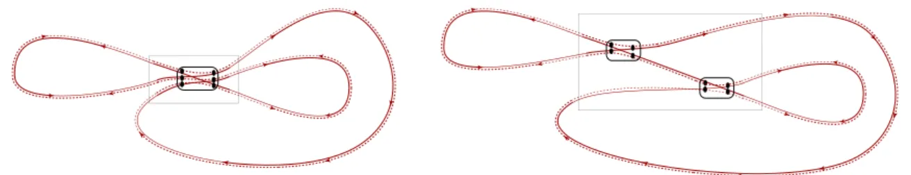
²

+ · · · . (1.5) At higher orders in the τ–expansion, orbit pairs of more complex topology enter the stage. (For some families of pairs contributing to the next–to–leading correction, K

sc⁽³⁾

, see figure 1.2.) The summation over all these pairs [23] — feasible under the presumed condition t > t

mix

— obtains an infinite τ –series which equals the series expansion of the RMT result (1.5). It is also noteworthy that both the topology of the contributing orbit pairs and the combinatorial aspects of the summation are in one–to–one correspondence to the impurity–diagram expansion [48] of the spectral correlation function of disordered quantum systems.

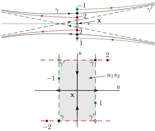
¹²

Central to our comparison of semiclassics and field theory below will be the un- derstanding of the encounter regions where formerly pairwise aligned orbit stretches reorganize. The analysis of these objects is greatly facilitated by switching from the con- figuration space representation originally used by SR to one in phase space [19, 20, 21].

In the following we briefly discuss the phase space structure of the regions where peri- odic orbits rearrange. In chapter 5 we will compare these structures to the (somewhat

11

For the sake of completeness, we report the full random matrix result, which reads

K

_RMT

(τ) =

( 2τ − τ ln(1 + 2τ), τ < 1, 2 − τ ln

^2τ+1_2τ−1

, τ > 1 in the orthogonal case, while in the unitary case the form factor is given by

K

RMT

(τ) =

( τ, τ < 1, 1, τ > 1.

12

Due to the notorious non–analyticity of K

RMT

(τ) at τ = 1 [3], the form factor at times τ > 1 was until very recently believed to be beyond the reach of semiclassical summation schemes. For τ > 1, however, there is another expansion scheme which is organized in terms of orbit/‘pseudo–orbit’ pairs and yields the τ > 1 expansion of the form factor [25]. These orbit/pseudo–orbit pairs have also been shown to be related term by term to a disorder diagram expansion about an additional ‘non–standard’

saddle–point.

(14)

Figure 1.2: Cartoon of three classes of orbit pairs that contribute to the expansion of the form factor at order τ

³

. (The triple–encounter region shown in the two figures on the right is the analog of the Hikami hexagon familiar from the impurity diagram approach to disordered systems.) The existence of the middle pair does not rely on time reversal invariance.

different) field theoretical variant of encounter processes.

Considering the correction K

sc⁽²⁾

as an example, we note that the encounter region contains four orbit stretches in close proximity to each other (cf. figures 1.1, 1.3): two segments x(t

₁

) and x

⁰

(t

₁

) of the orbits γ and γ

⁰

traversing the encounter region and the (close to) time reversed

¹³

x(t

₁

+ t

₂

) and x

⁰

(t

₁

+ t

₂

) of these trajectory segments reentering after one of the loops adjacent to the encounter region has been traversed (t

₂

is the duration of the loop traversal, and t

₁

parameterizes the time during which the encounter region is passed). To describe the dynamics of these trajectory segments, it is convenient to introduce a Poincar´ e surface of section S transverse to the trajectory x(t

₁

). For the sake of simplicity, let us consider a system with two degrees of freedom (a billiard, say), in which case S is a two–dimensional plane slicing through the three–

dimensional subspace of constant energy in phase space. We chose the origin of S such that it coincides with x(t

₁

). Introducing coordinate vectors e

_u

and e

_s

along the stable and unstable direction in S, the three points x(t ¯

₁

+ t

₂

), x

⁰

(t

₁

) and x ¯

⁰

(t

₁

+ t

₂

) are then represented by the coordinate pairs (u, s), (u, 0), and (0, s), respectively. (Notice that the trajectory γ

⁰

/T γ

⁰

traverses the encounter region on the unstable (s = 0)/stable (u = 0) manifold thus deviating from/approaching the reference orbit γ.)

s

u

x(t1)

t

enc

t

in

t

out

γ

γ⁰

x⁰(t1) γ⁰

x(t1) x⁰(t1)

¯ x(t1+t2)

¯ x⁰(t1+t2)

x⁰(t1+t2) x(t1+t2)

Figure 1.3: The structure of the encounter region. The picture on the right shows how the parallelogram spanned by the four points evolves in time t

₁

, while its symplectic area us is conserved.

The above coordinate system is optimally adjusted to a description of the two main characteristics of the encounter region: its duration t

_enc

and the action difference S

_γ

−S

_γ⁰

. Indeed, it is straightforward to show that the total action difference is simply given by the area of the parallelogram spanned by the four reference points in phase space,

13

In a position–momentum representation, x = (q, p), time reversal is defined as x ¯ ≡ (q, −p).

(15)

1.3 Quantum interference: Semiclassical background 15

S

_γ

− S

_γ⁰

= us [21]. As for the encounter duration, let us assume that the distance between the orbit points may grow up to a value c before they leave what we call the

‘encounter region’. (It is natural to identify c with the typical phase space scale up to which the dynamics can be linearized around x(t

₁

); however, any other classical scale will be just as good.) After the trajectory γ has entered the encounter region, it takes a time t

in

∼ λ

⁻¹

ln(c/s) to reach the surface of section and then a time t

out

∼ λ

⁻¹

ln(c/u) to continue to the end of the encounter region. (Here, λ is the Lyapunov exponent of the system. Thanks to the assumption t

_mix

t

_E

, λ may be assumed to be a ‘self averaging quantity’, constant in phase space.) The total duration of the passage is thus given by t

_enc

(u, s) ≡ t

_out

+ t

_in

∼ λ

⁻¹

ln(c

²

/(us)). The action difference of orbit pairs contributing significantly to the double sum must be small, |S

_γ

− S

_γ⁰

| = us . ~ . Consequently, t

enc

& λ

⁻¹

ln(c

²

/ ~ ) ≡ t

E

, where t

E

is the Ehrenfest time introduced above.

(Notice that both S

_γ

− S

_γ⁰

and t

_enc

depend only on the product us. While the individual coordinates u and s depend on the positioning of the surface of section, their product us is a canonical invariant and, therefore, independent of the choice of S.)

Having discussed the microscopic structure of the encounter region, we next need to ask a question of statistical nature: given a long periodic orbit γ of total time t, what is the number N (u, s, t) du ds of encounter regions with Poincar´ e paramet- ers in [u, u + du] × [s, s + ds]? (To each of these encounter regions there will be exactly one topologically distinct partner orbit γ

⁰

that is identical to γ in all other (N − 1) encounters. Thus, N (u, s, t) du ds is the number of SR pairs for a given parameter configuration and R

du ds N (u, s, t) is the total number of SR pairs.) Since the times t

₁

and t

₂

defining the two traversals of the encounter region are arbitrary (except for the obvious condition |t

₁

− t

₂

| > t

_enc

), N is proportional to the double integral N (u, s, t) du ds ∝

¹₂

R

t

0,|t₂−t₁|>t_enc

dt

₁

dt

₂

P

_ret

(u, s, t

₂

) du ds. The integrand P

_ret

is the probability to propagate from point (0, 0) in the Poincar´ e section to the time reverse of (u, s) in the time t

₂

. Since t

₂

> t

_enc

t

_mix

, this probability is constant and equals the inverse of the volume Ω = 2π ~ t

_H

of the energy shell, P

_ret

(u, s, t

₂

) = Ω

⁻¹

. Thanks to the constancy of P

_ret

, the temporal integrals can be performed and we obtain N (u, s, t) ∝ t(t − 2t

enc

)/(2Ω). The normalization of N is fixed by noting that the temporal double integral weighs each encounter event with a factor t

_enc

. The appropri- ately normalized number of encounters thus reads N (u, s) =

^t(t−2t_2t ^enc⁾

encΩ

. Substitution of N (u, s, t) into the Gutzwiller sum obtains

K

⁽²⁾

(τ ) = X

γ

|A

_γ

|

²

δ τ − T

_γ

t

_H

Z

c

−c

du ds N (u, s, t)2 cos(us/ ~ )

= τ

²

2π ~

Z

c

−c

du ds t

t

_enc

(u, s) − 2

cos(us/ ~ )

^~

=

^→0

−2τ

²

, (1.6) where we used the sum rule P

γ

|A

_γ

|

²

δ(τ − T

_γ

/t

_H

) = τ of Hannay and Ozorio de Almeida [49] and noted that in the semiclassical limit the first term in the integrand does not contribute (due to the singular dependence of t

_enc

on ~ ).

Before closing this section, let us discuss one last point related to the semiclassical

approach: the analysis above hinges on the ansatz made for the classical transition

probability P

_t

(x, x

⁰

) between different points in phase space. Specifically, a na¨ıve inter-

pretation of ergodicity — P

_t

(x, x

⁰

) = Ω

⁻¹

= const. for times t > t

_mix

— is too crude

(16)

to obtain a physically meaningful picture of weak localization. One rather has to take into account that the unstable coordinate, u(t), separating two initially close (u(0) c) points x and x

⁰

grows as u(t) ∼ u(0) exp(λt). For sufficiently small initial separation, the time it takes before the region of local linearizability is left,

1

2

t

_E

(x, x

⁰

) ≡ 1 λ ln c

u(0) , (1.7)

may well be larger than t

mix

. This is important because during the process of exponential divergence, the probability to propagate from x to the time reverse ¯ x

⁰

is identically zero.

(Simply because the proximity of x and x

⁰

implies that x and x ¯

⁰

are far away from each other.) Only after the domain of linearizable dynamics has been left, this quantity becomes finite and, in fact, constant:

P

t

(x, x ¯

⁰

) = 1

Ω Θ t − t

E

(x, x

⁰

)

, if |x − x

⁰

| c. (1.8) This concludes our brief survey of the semiclassical approach to quantum coherence. It will be the purpose of this thesis to discuss the corresponding field theoretical formulation.

By chapter 5, we will have obtained a sufficient grip on the field theory to discuss its structural parallels to the semiclassical formalism just presented.

1.4 Outline of this thesis

In chapter 2 we start out reviewing the known facts about the field theory approach to quantum chaos. Since the field theory in question — the ballistic σ–model — is plagued by a number of problems, we will stress the delicate points which were missed to date. Doing so, we show how to solve some of these problems in chapters 3 and 4.

As our knowledge how to evaluate the field theory grows, applications are discussed along the way. In particular, we present a consistent semiclassical approach to the proximity effect in chapter 3. We give an explanation of the proximity gap in chaotic SN structures and confirm the conjecture by LN that the width of this gap is set by the inverse Ehrenfest time. Chapter 4 is dedicated to developing a consistent evaluation scheme of the ballistic σ–model based upon a regularization procedure. We show how a variant of the BGS conjecture may be derived from first principles, which does not hold for individual systems, but rather for an ensemble of quantum systems which share the same classical limit. In chapter 5, we show how the quantum interference corrections to universal statistics found by the Haake group [24] are obtained from the field theory.

We take this example to explain how the field theory approach presented in this thesis

compares to the semiclassical approach which we discussed in section 1.3. We draw our

conclusions and give an outlook in chapter 6.

(17)

Chapter 2 Field theory: The ballistic σ σ σ–model

In this chapter we review the original derivation of the ballistic σ–model by Andreev et al. in the seminal papers [28, 29]. We lay particular emphasis on the subtleties which one might miss when extracting a semiclassical theory from an underlying quantum theory and which were overlooked by the original authors. We close with a discussion of the principal and ostensible problems of the ballistic σ–model which kept and keep puzzling the semiclassical and condensed matter community to date.

2.1 Derivation of the effective field theory

This introductory section consists of a review of the standard derivation of the ballistic σ–model by Andreev et al. until the point where the authors introduce the quasiclassical approximation. Starting from rather general assumptions, we obtain an effective (still quantum) field theory.

2.1.1 Representation of observables: An example

Since it is our aim to apply field theoretical methods to examine spectral properties we have to give a representation of spectral quantities amenable to field theory. To that end we write

ρ(E ) = 1

π Im tr G

⁻

(E) = 1

2πi tr G

⁻

(E) − G

⁺

(E)

, (2.1)

for the DoS, where the generalized retarded (+) and advanced (−) Green functions are defined as

G

^±

(E) ≡ E − H ± i0)

⁻¹

. (2.2)

In order to obtain a field theoretical representation we employ the generating functional

¹

Z(E, ω) ≡

Z

D[ ¯ ψ, ψ ] e

ⁱ^ψG^¯ ⁻¹^(E)ψ

, G

⁻¹

(E) ≡ E −

¹₂

ω

⁺

σ

₃^ar

− H, (2.3) where the ψ–fields are Grassmann–valued vectors in advanced/retarded (ar), N –dimen- sional Hilbert space, and R–dimensional replica space; since observables are represented

1

As a side remark, we mention that for discrete time quantum maps it is possible to formulate an analogous field theory by means of the color–flavor transformation [50].

17

(18)

by logarithmic derivates of the generating functional, the auxiliary R–fold replication of the theory serves to ensure proper normalization by means of the identity

ln z = lim

R→0

z

^R

− 1 R .

As an example of relevance to us, we want to consider the spectral two–point correlation function, R

₂

, which was defined in (1.1a). In terms of Green functions, R

₂

can be represented as

R

2

(ω) = ∆

²

2π

²

Re

tr G

⁺

(E + ω/2) tr G

⁻

(E − ω/2)

E,c

, where

AB

c

≡

AB

− A

B

denotes the connected average. To derive this representation from (2.1) we used that

G

⁺

(E

₁

)G

⁺

(E

₂

)

E

=

G

⁺

(E

₁

)

E

G

⁺

(E

₂

)

E

(and + −). R

₂

is then obtained by two–fold differentiation of the averaged generating functional, Z(ω) ≡

Z(E, ω)

E

, according to R

₂

(ω) = − ∆

²

2π

²

lim

R→0

1 R

²

Re ∂

²_ω

Z(ω).

This follows from the fact that (by construction) Z (ω

₁

− ω

₂

) =

det[iG

⁺

(E + ω

₁

)]

^R

det[iG

⁻

(E + ω

₂

)]

^R

E

. It is then straightforward to verify that

R→0

lim 1

R

²

Re ∂

_ω²

1−ω₂

Z(ω

₁

− ω

₂

) = − Re

tr G

⁺

(E + ω

₁

) tr G

⁻

(E + ω

₂

)

E,c

= − 2π

²

∆

²

R

2

(ω

1

− ω

2

).

In terms of the dimensionless variables s ≡ πω/∆ and τ ≡ t/t

H

, the field theoretical representations of R

₂

and the form factor read

R

₂

(s) = − lim

R→0

1 R

²

Re ∂

_s²

Z(s), (2.4a) K(τ ) = (2τ)

²

lim

R→0

1 R

²

Re Z(τ ). (2.4b)

2.1.2 Energy average

Given the conditions that the width E

_av

of the energy window is much larger than ∆ yet much smaller than the width of the spectrum, R

₂

is translationally invariant under shifts of the center–of–mass energy E within this window, and therefore the result does not depend on the precise form of the distribution which is used to perform the energy average in (1.1a). Assuming these conditions to be given we are thus free to employ a Gaussian average,

· · ·

E

= (2πE

_av²

)

⁻¹²

Z

dE e

⁻¹²

(

^E−EEav⁰

)

²

(· · · ), (2.5)

(19)

2.1 Derivation of the effective field theory 19

which induces an interaction term ∝ ( ¯ ψψ)

²

, Z(ω) =

Z

D[ ¯ ψ, ψ] e

ⁱ^ψG^¯ ⁻¹^(E⁰^)ψ−^E

2av 2 ( ¯ψψ)²

.

The interaction term is invariant under unitary transformations

ψ 7→ T ψ, ψ ¯ 7→ ψT ¯

^†

, T ∈ U(2RN

²

), (2.6) a symmetry which is broken by the other terms in the action, ω · ψσ ¯

₃^ar

ψ and ψHψ. We ¯ may decouple the interaction by means of a Hubbard–Stratonovich transformation

²

e

⁻^E

av2

2 ( ¯ψψ)²

= Z

D Qe ˜

⁻¹²^{tr ˜}^Q²^+E^av^ψ^¯^Qψ^˜

.

The invariance of the interaction term has to be respected by the term ψ ¯ Qψ. Accordingly, ˜ the symmetry transformation (2.6) induces the transformation

Q 7→ T ˜ QT ˜

⁻¹

on the Hubbard–Stratonovich field Q. Performing the (now Gaussian) integral over the ˜ ψ–fields we find that the partition function is given by

Z(ω) = Z

D Q ˜ e

⁻¹²^{tr ˜}^Q²^{+tr ln(G}⁻¹^{[ ˜}^Q]−¹²^ω⁺^σ³^ar⁾

, G

⁻¹

[ ˜ Q] ≡ E

₀

− H − iE

_av

Q. ˜ (2.7)

2.1.3 Saddle–point equation

Varying the action of the effective generating functional (2.7) w.r.t. Q ˜ and neglecting terms of order ω, one obtains the saddle–point equation

Q ˜

₀

= −iE

_av

G[ ˜ Q

₀

]. (2.8)

Applying an ansatz for Q ˜

₀

which is diagonal in the ‘internal’ (that is, all but the Hilbert space) indices, one finds the solutions

Q ˜

₀

(H) = −i E

0

− H 2E

_av

+ Λ

r

1 − E

0

− H 2E

_av

2

,

where Λ is an arbitrary traceless diagonal matrix with entries ±1.

2.1.4 Effective field theory

These solutions are in fact but some of a whole manifold of solutions, which is understood as follows: as we have seen above, the Q-field transforms according to ˜ Q 7→ T ˜ QT ˜

⁻¹

. We see that for ω = 0, the subgroup of transformations for which [H, T ] = 0 leaves the action invariant. Hence, for ω = 0, these transformations give rise to a whole manifold of saddle–points. If ω or [H, T ] are non–zero, the T -fields generate the low–energy

2

The missing i in the decoupled term is due to the anticommutativity of Grassmann fields,

viz. − tr( ¯ ψψ)

²

= + tr(ψ ψ) ¯

²

, which is decoupled as − tr( ˜ Qψ ψ) = ¯ ¯ ψ Qψ. ˜

(20)

configurations Q ˜ = T Q ˜

₀

T

⁻¹

. The transformations for which [T , Q ˜

₀

] = 0 have to be factored out since these do not give rise to new configurations Q. We note that ˜ the first term of Q ˜

0

is diagonal in the internal indices and therefore contributes only a constant to the soft mode action and that configurations with matrix elements T

_αα⁰

for which |E

₀

− E

_α

| > 2E

_av

result in a purely imaginary contribution which is exponentially suppressed. It is therefore allowed to effectively replace the saddle–point by

Q ˜

0

(H) = πE

av

Λδ

Eav

E

0

− H

, δ

Eav

(E ) ≡ 1 πE

_av

Re

r

1 − E 2E

_av

2

. (2.9)

The ‘delta function’ is in fact a normalized semicircle distribution and E

_av

denotes (a quarter of) its width. Keeping only the configurations which are soft and do not leave Q ˜

₀

invariant, the effective action reads (modulo inessential additive constants)

S[T ] = − β

2 tr ln G

⁻¹

[ ˜ Q] −

¹₂

ω

⁺

σ

^ar₃

= − β

2 tr ln G

⁻¹

[ ˜ Q

₀

] −

¹₂

ω

⁺

T

⁻¹

σ

₃^ar

T − T

⁻¹

[H, T ]

. (2.10)

For the explanation of the factor of β/2, note that we so far only considered the case of no discrete symmetries whatsoever (unitary symmetry class, β = 2). In appendix B we review the necessary modifications to take time reversal invariance into account (orthogonal symmetry class, β = 1), which roughly speaking leads to another doubling of field space by a ‘time reversal’ (tr) sector and an additional symmetry obeyed by the fields.

³

Further evaluation of this effective quantum field theory is possible only with additional assumptions as will become clear momentarily.

2.2 Semiclassical representation

This rather formal section serves to introduce a semiclassical expansion scheme of quantum theories which will later be employed to semiclassically evaluate the quantum action (2.10). The insights gained are nevertheless crucial for this work since they lay the ground for an adequate treatment of quantum uncertainty and other subtleties which tended to be obfuscated in the conventional field theory approach to quantum chaos.

2.2.1 Stratonovich–Weyl correspondence

A Stratonovich–Weyl correspondence is a family (parameterized by s ∈ R ) of one–to–

one linear maps associating to each Hilbert space operator A a function f

_A^(s)

on phase space Γ — called the symbol of the operator A — satisfying

(i) f

_A^(s)†

= f

_A^(s)

^∗

(reality) (ii) R

dx f

_A^(s)

(x) = tr A (standardization)

(iii) R

dx f

_A^(s)

(x)f

_B^(−s)

(x) = tr(AB) (traciality)

3

For more complicated symmetry classes we refer the reader to [51].

(21)

2.2 Semiclassical representation 21

along with covariance properties ensuring that the symbols transform properly when a quantum mechanical system is rotated, boosted, etc. [52, 53]. These conditions ensure that quantum mechanical expectation values — which are of the form tr(ρA) — may be interpreted as statistical expectation values of phase space observables. Together with traciality, standardization ensures that the unit operator is mapped to the constant function 1.

⁴

The operator product maps to the star product

f

_A^(s)

? f

_B^(s)

(x) ≡ f

_AB^(s)

(x).

Being the symbol of an operator product, the star product inherits associativity and non–commutativity.

2.2.2 Standard phase space and the Wigner symbol

In the remainder of this work we want to restrict ourselves to standard phase space Γ = R

^f

× R

^f

. The general case is discussed in [53] and applies, e.g., to the case Γ = S

²

of quantum mechanical spin [54]. We want to parameterize Γ using rescaled dimensionless phase space variables,

x = q

p

7→

q/q

₀

p/p

₀

,

which we will again denote by x. Here, q

₀

(p

₀

) is some classical and otherwise inessential constant of dimension length (momentum), say the system size (Fermi momentum).

Whenever we talk about ~ in the following we actually mean ~

eff

≡ ~ /(q

₀

p

₀

). This non–canonical rescaling allows a notion of Euclidean distance on phase space,

⁵

|x − x

⁰

| ≡ p

(q − q

⁰

)

²

+ (p − p

⁰

)

²

.

While the s 6= 0 members of the Stratonovich–Weyl correspondence for standard phase space are of importance in different contexts as well,

⁶

we will only make use of the s = 0 member, the so–called Wigner symbol

A(x) = Z

d∆q e

⁻^~ⁱ^p·∆q

hq +

¹₂

∆q|A|q −

¹₂

∆qi. (2.11) The corresponding star product is called Moyal product [56] and affords the two altern- ative representations

⁷

(AB)(x) =

Z dx

1

(π ~ )

^f

dx

2

(π ~ )

^f

e

²ⁱ^~^x^T¹^Ix²

A(x + x

₁

)B (x + x

₂

) (2.12a)

= A(x)e

^i~²

←−

∂_x^TI−→

∂x

B(x), (2.12b)

4

The phase space integral is normalized to unity.

5

Due to the Theorem of Darboux [55], there exist coordinates such that the symplectic form reads ω = P

i

dq

_i

∧ dp

_i

, which induces a Euclidean metric.

6

In particular, the (s = ±1)–pair of Husimi and Cahill–Glauber symbols.

7

These and other properties of the Wigner symbol are verified in appendix C.

(22)

where I ≡ (

₋₁¹

) is the symplectic unit operator. To obtain a convenient representation of the product of more than two operators, we iteratively apply the prototype formula equation (2.12a). A straightforward calculation then yields the general product formula

(A

₁

· · · A

_2n

)(x) = Z

²ⁿ

Y

i=1

dx

i

(π ~ )

^f

e

^~ⁱ^S(x¹^,...,x²ⁿ⁾

A

₁

(x + x

₁

) · · · A

_2n

(x + x

_2n

), (2.13) where the multilinear form S(x

₁

, . . . , x

_2n

) ≡ 2 P

i<j

(−)

^i+j+1

x

^T_i

Ix

_j

. A view at (2.12a) reveals that the oscillatory term kills all contributions outside a box where x

^T_i

Ix

_j

. ~ , i.e. it nails the phase space arguments onto each other only in the semiclassical limit

~ → 0. One of the most important messages to take home from this work may be formulated at this early stage already: the fuzziness of the coordinates in the Moyal product formula (2.12a) at finite values of ~ stems from the non–commutativity of quantum operator products and is therefore a direct manifestation of the uncertainty principle. Finally, the Moyal commutator is given by

[A, B ]

(x) = 2iA(x) sin ~ 2

← −

∂

_x^T

I − →

∂

_x

B (x)

= i ~ {A(x), B(x)} + . . . , (2.14) where {f, g}

x

is the Poisson bracket. A priori, the omitted terms are by no means small. This apparently trivial point and the quantum uncertainty inherent to the Moyal product have already been understood in several different contexts [57, 58, 59, 60]. They have nevertheless so far been overlooked in the semiclassical treatment of the ballistic σ–model; yet, they are crucial for its adequate derivation and evaluation. In that sense it is fair to call them novel achievements of this thesis, a predicate which also applies to the findings in the following subsections which deal with the regularity properties of the field degrees of freedom.

2.2.3 Off–shell structure of the fields

With this background we are in shape to construct a semiclassical representation of the action (2.10). To that end let us decompose phase space into one energy variable E = H(x) and (2f − 1) variables which parameterize the shells Γ(E) of constant energy E. According to the Theorem of Darboux, it is locally possible to decompose these variables into one variable t canonically conjugate to E which represents the travel time along the flow and 2(f − 1) canonical pairs denoted by y = (u, s) (standing for unstable/stable) which parameterize the cross–section transversal to the flow. These coordinates are taylor–made to reveal the features of the Hamiltonian flow.

Let us now turn to the phase space structure of the fields T rotating the reference point Q ˜

₀

in (2.9). We start out representing these fields as T = 1 1 + W, where the generators W obey the condition [W , Q ˜

₀

]

₊

= 0 (since a component commuting with Q ˜

₀

would not effect a rotation). Choosing [W, Λ]

₊

= 0,

⁸

it follows that W has to commute with the Hilbert space content of Q ˜

₀

, [W, δ

_E_av

(E

₀

− H)] = 0. Using the Moyal product formula (2.12a) plus the decomposition x

^T₁

I x

₂

= y

^T₁

Iy

₂

+E

₁

t

₂

− E

₂

t

₁

of the symplectic

8

That is, W is block off–diagonal w.r.t. an ordering (+1, . . . , +1, −1, . . . , −1) of the entries of Λ.

(23)

2.2 Semiclassical representation 23

product, and transforming to a frequency representation, f () ≡ (2π ~ )

⁻¹

R

dt e

^~ⁱ^t

f(t), it is straightforward to verify that

δ

_E_av

(E

₀

− H)W

(E, , y) = W(E, , y)δ

_E_av

2 − (E − E

₀

) Wδ

_E_av

(E

₀

− H)](E, , y) = W(E, , y)δ

_E_av

2 + (E − E

₀

) .

Obviously, only those generators span up the field manifold which do not annihilate the saddle–point, implying that neither of these terms must vanish. On the other hand, the commutator [δ

Eav

(E

0

− H), W] does have to vanish, that is

0 = W(E, , y) n δ

_E_av

2 − (E − E

₀

)

− δ

_E_av

2 + (E − E

₀

) o .

Taken together, these requirements amount to the restrictions

|E − E

₀

| ≤ E

_av

, || ≤ E

_av

− |(E − E

₀

)| ≤ E

_av

,

which are easily verified to carry over to arbitrary powers of W. Altogether, we see that a given width E

av

of the energy window does not only nail the support of the fields down to a window of width of order E

_av

about the energy shell; it also induces an uncertainty of the T –fields in the t–direction on the scale t

_av

≡ 2π ~ /E

_av

. In order to resolve all details, t

av

necessarily has to be smaller than any other relevant time scale of the system. Since the smallest such time scale is certainly classical (typically, it is set by the Lyapunov time t

_L

), it suffices to take t

_av

much smaller yet still classical. We then find that averaging over an energy window as narrow as E

av

∼ ~ suffices to resolve all details of interest, and we will stick to this choice throughout the remainder of this work.

⁹

2.2.4 Regularity of the field space

Having understood that all Wigner symbols appearing in the action (2.10) are confined to a small neighborhood of the energy shell, the following important observation applies:

let the support of both A(x) and (AB)(x) be classically finite. Then, the Moyal product effects a smoothing of scales scaling smaller than ~ . To see this, define the convolution of an operator A with a Gaussian,

A

~^α

(x) = Z

dx

⁰

A(x

⁰

)g

_~^α

(x − x

⁰

),

where g

_~^α

stands for a unit normalized isotropic Gaussian with width σ ∼ ~

^α

. It is then easy to see that the Moyal product is invariant under smoothing in the sense that

AB = A B

~^α

= AB

~^α

, α > 1. (2.15)

9

In contrast to our findings, Efetov et al. [61] obtain an infinitely thin energy shell. It is unclear to

us how the authors can do so without losing the resolution in direction of the flow.

(24)

This is shown as follows: an application of the integral formula (2.12a) gives A

B

~^α

(x) =

Z dx

₁

(π ~ )

^f

dx

₂

(π ~ )

^f

Z

dx

⁰

e

²ⁱ^~^x^T¹^Ix²

A(x + x

₁

)B (x

⁰

)g

_~^α

(x + x

₂

− x

⁰

)

=

Z dx

₁

(π ~ )

^f

dx

⁰

(π ~ )

^f

e

²ⁱ^~^x^T¹^I(x⁰^−x)

A(x + x

₁

)B (x

⁰

) Z

dx

₂

e

²ⁱ^~^x^T¹^Ix²

g

_~^α

(x

₂

)

=

Z dx

₁

(π ~ )

^f

dx

⁰

(π ~ )

^f

e

²ⁱ^~^x^T¹^Ix⁰

A(x + x

₁

)B(x + x

⁰

)e

^−(x¹^~^α−1⁾²

= (AB)(x).

These equations should be read bottom up. In the crucial last line, finiteness of x and x+ x

₁

implies that x

₁

is also finite, which in turn means (since α > 1) that the Gaussian is effectively unity. Summarizing, we may a priori restrict ourselves to a field space consisting only of those Wigner symbols which display no features smaller than ~ .

2.3 The ballistic σ σ σ–model

Having understood about the subtleties of the Wigner representation we now continue our review of the derivation by Andreev et al. We start out with a bona fide review of their last steps towards the ballistic σ–model (2.18); this serves to put the reader into the position of the perplexed reader of the original works. After a discussion of the problems of which the ballistic σ–model suffers if taken at face value, we outline how a regularization scheme would resolve one major drawback.

2.3.1 The original derivation of the ballistic σ σ σ–model

Let us assume that an (a priori formal) expansion of the effective action (2.10) in the terms ω tr(σ

₃^ar

Q) ˜ and [H, T ] that break the symmetry of the action is justified. We are then led to

S

₀

[T ] = iβπ 2∆

Z dx

Ω tr

¹₂

ω

⁺

σ

₃^ar

Q − T Q

₀

[H, T

⁻¹

] ,

where use of Weyl’s law Ω∆ = (2π ~ )

^f

was made and all products are understood as Moyal products. We further made use of the saddle–point equation (2.8), and spurious normalization factors were absorbed by letting

Q ≡ (πE

_av

)

⁻¹

Q. ˜ (2.16)

Let us further assume that the commutator can be replaced by the Poison bracket according to

[H, T

⁻¹

] 7→ i ~ {H, T

⁻¹

}. (2.17) This replacement results from a (once again just formal) truncation of the expansion (2.14) at first order. In addition — and, as will turn out shortly, closely related to the

‘quasiclassical’ truncation (2.17) — let us assume ‘mode locking’, i.e. that the fields T (x) do not depend on the energy variable E = H(x) on their support (which is concentrated to the energy shell of classically vanishing width E

A Field Theory Approach to Universality in Quantum Chaos