photon-dominated clouds in NGC 3603

The physics and chemistry of

photon-dominated clouds in NGC 3603

Inaugural-Dissertation

zur

Erlangung des Doktorgrades

der Mathematisch-Naturwissenschaftlichen Fakultät der Universität zu Köln

vorgelegt von Zoltán Sándor Makai

aus Budapest

Köln 2014

Tag der mündlichen Prüfung: 14. Oktober 2014.

For Andi

and

for the memory of my parents

Mom (†2008) and Dad (†2013)

stars. Therefore, in order to make an apple pie from scratch, you must first create the universe. We are made of starstuff.”

Carl Edward Sagan

“Not only is the Universe stranger than we think, it is stranger than we can think.”

Werner Heisenberg

“A sok tudás nem tanít meg a helyes gondolkodásra”

Herakleitosz

Contents

Abstract 1

Kurzzusammenfassung 2

1 Introduction 5

1.1 Motivation . . . . 6

2 Theoretical background 11 2.1 Spectral features . . . . 11

2.1.1 Rotational lines . . . . 11

2.1.2 Fine- and hyperfine-structures . . . . 12

2.2 Einstein–coefficients and critical density . . . . 12

2.3 Radiative transfer . . . . 15

2.4 Optical depth and column density calculation . . . . 16

2.5 Photon-Dominated Regions (PDRs) . . . . 18

2.5.1 Energy balance . . . . 19

Heating . . . . 19

Cooling . . . . 21

2.6 Chemistry in the ISM . . . . 22

2.6.1 Gas phase chemistry . . . . 22

2.6.2 Grain surface chemistry . . . . 23

3 Observations by the Herschel Space Observatory 25

3.1 The Herschel Space Observatory . . . . 25

3.1.1 HIFI . . . . 26

Observing modes with HIFI . . . . 26

3.1.2 PACS . . . . 29

Observing modes with PACS . . . . 30

3.1.3 SPIRE . . . . 30

3.2 The WADI key–project . . . . 32

3.2.1 The target source: NGC 3603 . . . . 32

4 Data reduction 39 4.1 HIPE . . . . 39

4.1.1 HIFI pipeline processes . . . . 40

4.1.2 PACS pipeline processes . . . . 40

4.2 CLASS . . . . 41

4.3 Summary . . . . 44

5 Complementary data 47 5.1 SEST data . . . . 47

5.2 NANTEN2 data . . . . 49

5.3 PACS and SPIRE data (Hi-GAL survey) . . . . 50

6 Observational results 55 6.1 Integrated intensity maps . . . . 55

6.1.1 HIFI OTF-maps . . . . 55

6.1.2 PACS-maps . . . . 57

Line spectroscopy . . . . 57

Range spectroscopy . . . . 58

6.2 Velocity structure and line shapes . . . . 60

6.2.1 Position–velocity diagrams . . . . 60

OTF observations . . . . 60

Cut observations . . . . 62

6.2.2 Channel maps . . . . 65

iii

6.2.3 Line profiles and intensities . . . . 66

OTF observations (C1, C2 and C3) . . . . 67

Cut observations . . . . 71

Point observations . . . . 74

6.2.4 Kinematic distance . . . . 78

6.3 Excitation temperature . . . . 79

6.4 Derivation of column densities . . . . 79

6.4.1 Column densities along C1, C2 and C3 (OTF-map) . 81 H

column density . . . . 81

6.4.2 Column densities from cut observations . . . . 83

6.4.3 Column densities from point observations . . . . 83

Abundances . . . . 85

6.5 Mass calculations . . . . 89

6.5.1 Total and virial gas masses . . . . 89

6.5.2 Jeans mass . . . . 91

6.6 Summary . . . . 93

7 Model results 95 7.1 Theory . . . . 95

7.1.1 The RADEX code . . . . 96

7.1.2 The KOSMA-τ PDR model . . . . 97

7.2 Results . . . . 99

7.2.1 RADEX . . . 100

7.2.2 KOSMA-τ . . . 101

7.3 Summary . . . 107

8 Interpretation and discussion 109 8.1 Gas motions . . . 109

8.1.1 Signatures of turbulence . . . 109

8.1.2 Footprints of rotation/torsion . . . 112

8.1.3 Internal cavity in MM2? . . . 114

8.2 Cloud (in)stability . . . 115

8.3 Embedded sources . . . 117

8.4 Density and UV-field with the KOSMA-τ model . . . 119

8.5 Density and temperature with the RADEX . . . 120

8.6 The I(

CO)/I(

CO) ratio . . . 122

8.7 Chemical stratification/structure of NGC 3603 . . . 124

8.7.1 Chemical abundances in NGC 3603 . . . 126

8.7.2 H

formation and destruction . . . 129

Summary 132 References 143 A Summary of HIFI data 155 B Summary of PACS data 159 C Comparison of Herschel and NANTEN2 intensity maps 161 D Line fits of the observed species from the OTF–map observa- tions 167 E Line fits of the observed species from the cut observations 179 E.1 1342201675 (o–H

O — MM1) . . . 179

E.2 1342201676 (o–H

O — MM2) . . . 180

E.3 1342201750 (

CO — MM1) . . . 181

E.4 1342201752 (

CO — MM2) . . . 182

E.5 1342201809 (

CO — MM1) . . . 184

E.6 1342201810 (

CO — MM2) . . . 185

E.7 1342201818 (

C

— MM1) . . . 186

E.8 1342201819 (

C

— MM2) . . . 188 F Line fits of the observed species from the point observations 191

G Velocity channel maps 195

H Line shapes and their distributions in MM1 and MM2 199

v I Integrated intensity maps of the observed species from PACS

observations 207

J The derived physical parameters for Herschel observations 213 K Energy level diagrams of the observed species 227

L Beam size correction 235

M Example scripts 239

List of Figures 251

List of Tables 257

Acknowledgements 259

Erklärung 263

Curriculum vitae 264

Abstract

High-mass star-formation in the interstellar medium is one of the main open questions in astronomy: high-mass stars are rare, evolve fast and are frequently obscured or located in dense clusters. Most of our knowl- edge stems from simulations, not from direct observations.

Stars are born within molecular clouds due to the perturbations of local physical and chemical processes. To investigate these perturbations, we observed one of the most prominent HII region, NGC 3603, in our Galaxy.

This molecular cloud complex embraces an open cluster, with massive and hot stars, which provides strong stellar winds and radiation field. These phenomena heavily interact with the neighbouring environment and gov- ern the local physics and chemistry.

To investigate these effects and their influence, we received spectroscopy data of molecules, ions and atoms via Herschel Space Observatory. Data of ground-based telescopes were also used as complementary data.

The observational results showed that the observed clouds have gas com- ponents with different temperatures as well as vigorous gas movements.

Different models were used to fit the observations. We found that the ob- served line intensities and abundances match with the model predictions and the model results are independent from the cloud geometry.

All the results we obtain, give the opportunity to characterize the physi- cal conditions and chemical processes within NGC 3603. Based on our observations and our model calculations, we concluded that the observed molecular clouds (or part of them) are probably in gravitationally unstable stage. Hence, the star-formation process within NGC 3603 is still ongoing.

This scenario is in agreement with previous studies. It is also likely, that

the observed clouds do not rotate as a rigid rotor but have a torsional ge-

ometry. On the other hand, due to observational facts (e.g., large beam

size, distance of NGC 3603), we were only be able to make statements

about the chemistry/chemical stratification within certain limits.

Kurzzusammenfassung

Die Entstehung massereicher Sterne ist eine der großen offenen Fragen moderner Astronomie. Massereiche Sterne sind selten, entwickeln sich schnell und sind oft tief in Staub eingebettet oder in dichten Sternhaufen zu finden. Der größte Teil unseres Wissens über massive Sternentstehung stammt daher aus Simulationen und nicht aus direkten Beobachtungen.

Lokale Störungen des physikalischen und chemischen Zustandes regen die Bildung von Sternen in Molekülwolken an. Um diese Störungen zu untersuchen beobachteten wir eine der prominentesten HII Regionen in- nerhalb unserer Milchstraße, NGC 3603. Dieser Molekülwolkenkomplex umgibt einen offenen Sternhaufen heißer massereicher Sterne die starke Sternwinde und intensive Strahlung produzieren.

Um deren Einfluß auf die Sternentstehung zu untersuchen, verwendeten wir spektroskopische Beobachtungen des Herschel Weltraumteleskops von Molekülen, Ionen und Atomen. Zusätzlich dazu haben wir komple- mentäre Daten bodengestützter Teleskope verwendet.

Die Daten zeigen, daß die beobachtenen Molekülwolken Gaskomponen- ten mit verschiedenen Temperaturen beherbergen, die teilweise starke Strömungsgeschwindigkeiten aufweisen.

Unsere Ergebnisse erlauben uns die physikalischen und chemischen Zu-

standsbedingungen innerhalb NGC 3603 zu charakterisieren. Basierend

auf unseren Beobachtungen und unseren Modellrechnungen schließen

wir, daß die beobachteten Molekülwolken (bzw. Teile von ihnen) gravitativ

instabil sind. Folglich ist von einer anhaltenden Sternentstehung in NGC

3603 auszugehen. Diese Annahme wir auch von früheren Studien unter-

stützt. Es ist weiterhin wahrscheinlich, daß die beobachteten Wolken nicht

starr rotieren, sondern eher eine torsionsartige Geometrie aufweisen. Die

große Entfernung von NGC 3603 sowie der endlich große Teleskopbeam

erlauben uns nur eingeschränkte Aussagen über die chemische Schich-

tung des lokalen Gases zu treffen.

1

Introduction

The history of observational radio astronomy goes back to the first third of 20

century (1930’s) when Karl Jansky was employed by the Bell Tele- phone Laboratory as an engineer and investigated statics of an antenna.

He detected an unknown periodic signal from the sky. He realized that the detected radiation originates from the Milky Way, more precisely from the Sagittarius constellation

(Jansky, 1933), in the direction of the center of our Galaxy. He also stated that the signals are probably emitted by the interstellar gas and dust, which is called interstellar medium (ISM).

A disadvantage of ground-based telescopes that operate in the radio regime is, that the Earth’s atmosphere acts as a filter which absorbs a specific frequency range toward the shorter wavelengths (to far-infrared and sub-millimeter regimes) from the sky (Fig. 1.1). Therefore, telescopes operating at this wavelength regimes are mounted at high elevations and dry locations [e.g. NANTEN2

telescope or ALMA

(altitude ∼ 5000 m at Atacama desert, Chile)]. Alternatively, telescopes are also placed above the atmospheric water [e.g. Stratospheric Observatory for Infrared Astron- omy (SOFIA)] or even above the atmosphere [Herschel Space Observa- tory (HSO)].

These highly sophisticated instruments allow us to make on an in-depth study and investigation of the radiation emitted by molecules, ions and atoms that play important roles in the physics and chemistry of the ISM.

1

At that time, Jansky did not know that the source of the detected signal is the Sagittarius-A itself.

2

NANTEN means “southern sky“ in Japanese

3

Atacama Large Millimeter/submillimeter Array

Figure 1.1: The Earth’s atmospheric transmission. Copyright: NASA.

1.1 Motivation

Our fundamental intention is to understand the main physical conditions and chemical processes in the ISM. One of the open problems in astron- omy is the high-mass star-formation. Stars are formed by collapse of cold and dense cores of molecular clouds that are probably fragmented from their parental molecular cloud. The fragmentations are caused by pertur- bations.

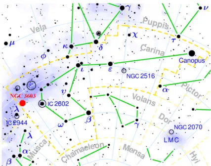
The method that we use to study the perturbations is to observe molecules, atoms and ions which are sensitive to these changes, and serve as tracers of their environment and its conditions that are dominant there. To study and understand the star-formation mechanism, we choose NGC 3603 which is one of the most luminous and prominent HII regions in our Galaxy, located in the Carina constellation (Fig. 1.2) visible only from the southern hemisphere. This object, which is a cloud complex, contains a massive star cluster that provides strong stellar winds and radiation fields which strongly interact with the adjacent environment.

The radiation heats up the surface of the closely located molecular clouds.

That warm and thin (compared to the size of the whole molecular cloud) transitional layer

, which is called Photon-Dominated Region (PDR

), is an extraordinary astrophysical laboratory where the local physical and chem-

4

We need to keep in mind, that the structure of the molecular clouds can be described by a fractal-Brownian-motion (fBm) Stutzki et al. (1998). Assuming that the three dimen- sional structure of a cloud can be described by an fBm structure, the volume is dominated by the cloud surface (the surface grows in proportion with the volume) and therefore, this

“thin surface layer” makes up a good fraction of the molecular material (Stutzki, 1999).

5

This thin layer is also referred as Photo-dissociation Region. I shall use abbreviation

PDR as Photon-Dominated Region.

1.1 Motivation 7

Figure 1.2: The position of NGC 3603 (filled red circle) in the Carina con- stellation on the southern hemisphere. Copyright: wikipedia.org

ical conditions are influenced and dominated by photons with defined en- ergy range (6 ≤ hν ≤ 13.6 eV)

.

As mentioned earlier, we need to investigate the different physical con- ditions and chemical processes through a group of carefully selected species (molecules, atoms and ions) that are sensible for the various den- sities and temperatures.

The footprints of these physical and chemical changes are manifested by either emissions or absorptions of the observed molecules, atoms and ions. Due to the complexity of the interstellar medium (including PDRs), we selected a few specific questions to better understand the physics and chemistry of the ISM.

• What is the distribution of dust temperature and how is N(H

) distributed around the central cluster?

Molecular hydrogen is the most abundant molecule in the interstellar medium. Because it efficiently forms on dust grain surfaces (within a certain dust temperature), dust is very important. It acts as cat- alysts for many chemical reactions [even though dust is much less abundant than gas (gas-to-dust mass ratio is ∼ 100)]. Thus, the in- vestigation of the dust and N(H

) distribution may lead to study the formation of molecular hydrogen.

• Are the observed molecular clouds at the gravitationally stable or unstable stage?

6

The 6 and 13.6 eV are the ionization potential of dust and hydrogen, respectively.

As I mentioned, stars are born in cold and dense cores which are deeply embedded in their host molecular clouds. These cores are created by fragmentation. For the existence of fragmentations, the molecular cloud has to be energetically unstable (the cloud is not in virial equilibrium) which means that the thermal (or kinetic) en- ergy and the gravitational potential energy compete with each other.

The comparison of the observational data to the virial theorem pro- vides us an insight into the stability of an observed cloud (more pre- cisely stability of any system), hence we can deduce whether the star-formation is still an ongoing process or not.

• Are there any observable signatures of systematic gas motions and/or enhanced turbulent?

Turbulence is a relevant trigger of star formation. Gas motions within a molecular cloud happen on large (Brunt et al., 2009) and small scales (Nakamura & Li, 2008; Wang et al., 2010). For example, shock fronts, which are pressure-driven waves that propagates into their neighbouring gas faster than the local sound speed, trigger the star formations. Therefore, the observations of the signatures of tur- bulence (e.g. broad line widths) could help to identify the existence of turbulence. The study of the velocity structure of the observed molecular cloud may give an insight to the dominant and/or turbulent gas motions.

• Is there any observable influence of prominent embedded in- frared sources on the physics and chemistry of the observed molecular clouds?

Photons within a certain energy range (6 eV ≤ hν ≤ 13.6 eV) are playing important role in the chemical and thermal balance of the PDRs. The birth places of these FUV-photons are high mass stars (O- and early B-type stars

) which could exist either outside or inside of a molecular cloud.

The local physics and chemistry may be governed by the embedded hot stars, hence the investigation of their adjacent environment could help to characterize the physics and chemistry inside the observed molecular cloud.

• Are the model predictions of line intensities and densities, and observations in good agreement?

We can prove our theoretical knowledge about the physical and chemical processes in the ISM with comparisons of observational data and model computations. Numerous models are exist with var- ious assumptions about geometry, physics and chemistry. To un-

7

The stars are classified based on their spectral characteristics and temperature. In

the Morgan–Keenen system, stars are denoted by letters from O, B, . . . M, L; from the

hottest to the coolest, respectively.

1.1 Motivation 9 derstand and give a well detailed description of the ISM is a heroic contention due to its complexity, hence it is beneficial to widen the statistical sample as much as possible to approximate the realness.

• Is there any observable chemical stratification? Are the ob- served abundances comparable with model predictions?

We presume that NGC 3603 contains PDRs [e.g. Röllig et al. (2011)]

which gives us an exceptional opportunity to study and compare the observations with the theoretical predictions. PDRs are consist of different layers where the physical conditions and chemical reactions are governed by the decreasing FUV-field strength as a function of cloud depth. Hence, the physical conditions and efficient chemical processes vary in the different layers. The investigation of chemical stratification may allow us to deduce the cloud structure.

Keeping these questions in mind, I shall present detailed study of dense gas tracers [Carbon Monosulfide

(CS) and Formyl ion (HCO

)], diffuse gas tracers [Ethynyl radical(C

H) and Methyladyne radical(CH)], shock tracer [Water (H

O)], important cooling lines (atomic and ionized oxygen [OI]

and [OIII], atomic and ionized carbon [CI] and [CII] . . . ) and the most abundant (after H

) Carbon Monoxide (

CO) lines (and its isotopologues,

13

CO and C

O) to help characterize the main physical conditions, and chemical processes in the prominent star-forming region NGC 3603.

8

For the nomenclature of molecules, ions and atoms I follow the book Tielens (2005).

9

The transitions denoted with square bracket (e.g. [CII]) signify forbidden transitions

which means no lines can be measured in earthly laboratories.

2

Theoretical background

We receive information about the physical conditions of the ISM via spec- tral line features. These features (either could be line emission or absorp- tion) reflect the physical conditions (density, temperature, pressure) in the molecular clouds. In this chapter, I briefly introduce the physical back- ground necessary for the following chapters. Further and well detailed dis- cussions of the theoretical background can be found in numerous books [for example, Draine (2011); Herzberg (1991, 2010); Rybicki & Lightman (2004); Tielens (2005); Wilson et al. (2009)].

2.1 Spectral features

We mostly receive information from the physical and chemical conditions of the ISM via line emissions (or absorption). To be able to observe this as- trophysical phenomena, a quantum-mechanical energy state of the emitter or absorber needs to be excited. The observed photon frequency (ν) corre- sponds to the energy difference between two states (∆E = hν). Because we observe emission from rotational lines, fine- and hyperfine-structures, I provide a very short introduction to the phenomenon that produce these lines.

2.1.1 Rotational lines

The spectral line features are results from quantum-mechanical molecu-

lar rotational transitions. Quantum mechanics allows rotating molecules

to possess only discrete quanta of angular momentum (due to the selec-

tion rules). The rotational energy is proportional to J (J + 1) which means

that the rotational transition frequency is related to J (ν ∼ J). Note, that

molecules without permanent electric dipole moment cannot have pure rotational transitions and I shall use the notation system J → J − 1 for rotational transitions

.

2.1.2 Fine- and hyperfine-structures

As an electron orbits around the nucleus (or nuclei in molecules) the mag- netic field of nucleus (or nuclei) interact with the magnetic moment gener- ated by the electron’s spin (due its intrinsic angular momentum). This con- nection slightly shifts the electron’s energy levels which can be detected as a split of the energy levels. This small (∼ 10

eV) splitting of a spectral line is called fine-structure split which is, again, a result of the interaction between a particle’s orbit and its spin.

It is possible that the fine-structure lines are further divided due to an- other quantum-mechanical effects. Not only the electrons but also the nucleus (or nuclei) possesses a spin, hence a magnetic moment, too. The magnetic moment of the nucleus (or nuclei) interacts with the previously mentioned electromagnetic fields and splits the fine-structure lines into en- ergy levels with even smaller energy difference than fine-structure levels (∼ 10

eV). This split is called hyperfine-structure.

2.2 Einstein–coefficients and critical density

As a first approximation, we assume a two-level system and these levels are occupied by n

and n

number of particles where the subscripts denote the energy levels (upper and lower)

. Under certain conditions, transitions between these two levels are possible with different probabilities. These probabilities are described by the Einstein-coefficients:

Spontaneous emission coefficient (A

[s

]) It gives the probability of spontaneous emission of a photon due to the transition from level u to l.

The number of radiative transitions per second per unit volume is A

n

.

Absorption coefficient (B

[s

erg

cm

sr]) The probability of ab- sorption of a photon (with frequency ν) by a particle that transits from level

1

For example, the rotational transition from the first excited state to the ground state of carbon monoxide is nominated as

CO (1 → 0).

2

The energy difference between the upper and lower levels is: E

− E

= hν.

2.2 Einstein–coefficients and critical density 13 l to u. The number of transitions per second per unit volume per unit mean intensity

is B

n

I

.

Induced emission coefficient (B

[s

erg

cm

sr]) The probability of stimulated emission of a photon (with frequency ν) by a particle that transits from level u to l. The number of radiative transitions per second per unit volume is B

n

I

.

These coefficients are connected to each other and the relationship can be written as:

B

B

= g

g

and A

= 8πhν

c

B

(2.1)

where h is the Planck-constant (h ≈ 6.63 × 10

m

kg s

), c ≈ 3 × 10

m s

is the speed of light in vacuum, g

and g

are the statistical weights of upper and lower energy levels, respectively. In local thermodynamic equilibrium (LTE), the populations of the upper and lower energy levels (n

and n

) are described by the Boltzman–distribution (with a temperature

that characterizes the population ratio) and proportional to the statistical weights of the energy levels:

n

n

= g

g

e

(2.2)

where k is the Boltzmann-constant (k ≈ 1.38 × 10

m

kg s

K

).

Collisional processes

In the interstellar medium, besides radiation, collisional excitations (and de-excitations) are important cooling and heating processes in the ISM. To get some impression about the prevailing excitation mechanisms (radiation or collisions), the interstellar gas density needs to be investigated. For this, we introduce the collision rates C

and C

for the lower and the upper energy levels, respectively:

C

=< σ

v > [cm

s

] (2.3) where σ

is the collisional cross section and v is the relative velocity of collisional partners. The number of collisional transitions per second per

3

We assume that a radiation field is exist with a mean intensity I which is described by the Planck-function (assuming thermodynamic equilibrium).

4

The temperature is either the kinetic temperature (T

) if collisions dominate (LTE)

or the radiation temperature (T

) if radiation dominates.

unit volume are n

C

and n

C

. In statistical equilibrium the number of upward and downward transitions are equal:

n

B

I

+ n

C

= n

A

+ n

B

I

+ n

C

(2.4) Thus, the ratio of level population

n

n

= B

I

+ C

A

+ B

I

+ C

(2.5) If we assume that the collisional excitation and de-excitation processes are dominant, and take into account that the level population follows the Boltzmann-distribution (in LTE), Eq. (2.5) becomes

n

n

= C

C

= g

g

e

(2.6)

If we use the relationships B

= (c

/8πhν

)A

, B

= B

(g

/g

) and C

= C

(g

/g

) exp(−hν/kT ), Eq. (2.5) can be written as:

n

n

= g

g

e

K I

(e

)

+ (C

/A

)

1 + K I

+ (C

/A

) (2.7) where K = c

/8πhν

. Using Eq. (2.3) we can write:

n

n

= C

A

where n

≡ A

C

≈ A

< σ v > [cm

] (2.8) The density value where the importance of collisional and radiative de- excitations are equal is called critical density. The critical density varies species by species and is different for each transition. If the gas density is larger than the critical density (n n

), collisions are the dominant exci- tation mechanism and the level population is described by the Boltzmann- distribution. In this case, the excitation temperature is equal to the kinetic temperature of the gas (T

= T

).

However, considering optical depth effect, critical density can be changed by a factor β(τ ). The factor β(τ ) originates from the escape probability theory which describes the chance that a photon formed at optical depth τ in a molecular cloud can leave/escape the cloud before being absorbed, and the critical density can be written as:

n

= A

C

β(τ

) [cm

] (2.9)

2.3 Radiative transfer 15 More detailed description of the connections between the gas and its criti- cal density can be found, for example, in Wilson et al. (2009) or e.g. discus- sion for optically thick case in Mihalas (1978); Scoville & Solomon (1974);

Stutzki & Winnewisser (1985).

2.3 Radiative transfer

Radiative transfer describing how radiation propagates in the ISM (consid- ering scattering by dust and gas, and emission and absorption processes).

The basic equation of radiative transfer is:

dI

ds = −κ

I

+

(2.10)

where I

is the specific intensity per unit time, surface, and solid angle in the frequency range of [ν, ν + dν], ds is the path length (or an infinitesimal step along the line of sight), κ

and

are the absorption and emission coefficient, respectively. They can be written as:

= hν

4π n

A

φ(ν) (2.11a)

κ

= hν

c (n

B

− n

B

)φ(ν) (2.11b) where φ(ν) is the normalized line profile function ( R

φ(ν)dν = 1) giving the probability of emitted photon is in the range of [ν, ν + dν]. Defining optical depth (dτ

= −κ

ds) and source function (S

=

/κ

) the Eq. (2.10) can be rewritten as:

dI

dτ

= −I

+ S

(2.12)

The general solution of this equation is:

I

(τ

) = I

(0)e

+

τν

Z

0

S

(τ

)e

dτ

(2.13)

It gives information about the background radiation (first part) and the radi-

ation which is emitted and absorbed by the medium (second part). Assum-

ing thermal equilibrium [dI

/ds = 0, (Wilson et al., 2009)], the distribution

of intensity is described by the Planck–function B

with a formal excitation

temperature (T

), and we can write:

I

= S

=

κ

= B

(T) = 2hν

c

1

e

− 1 (2.14)

If we assume a homogeneous medium, the solution of Eq. (2.13):

I

(τ

) = I

(0)e

+ S

(τ

)(1 − e

) (2.15) In radio astronomy, the received emission is often described in terms of the brightness temperature (T

= I

c

/2kν

). Hence the solution of radiative equation can be written using the brightness temperature:

T

(τ

) = T

(0)e

+ T

(τ

)(1 − e

) (2.16) where T

(0) is the temperature of the background. If the detected emis- sion is optically thick (τ

1), we observe the excitation temperature but in case of optically thin emission (τ

1) only T

= τ

T

is defined.

2.4 Optical depth and column density calcula- tion

In practice, we receive emitted photons not only from the observed source.

Spectral-line data often contain continuum sources (either from the target source or from nearby sources in the field of view). In a case where we are interested about spectral lines, the continuum level needs to be subtracted from the data set. Well detailed methods for continuum subtraction can be found in e.g. Wilson et al. (2009). With this, Eq. (2.16) can be written as:

J

(T

) = f[J

(T

) − J

(T

)](1 − e

) (2.17) where J

(T ) = (hν/k)[exp(hν/kT ) − 1]

is the normalized Planck–

intensity and f is the filling factor (which is a fraction of the telescope beam occupied by the observed source). The term T

denotes the temperature of the cosmic background radiation with a value 2.725 K (Fixsen, 2009).

Using the relationship between the Einstein–coefficients, the definitions of the emission and absorption coefficients (2.11a) and (2.11b), and the definition of the optical depth, τ

can be written as (for a given transition):

τ

= N

A

c

8πν

g

g

(1 − e

) (2.18)

where N

= R

n

ds is the column density of the upper level.

2.4 Optical depth and column density calculation 17 Considering optically thin emission [J

(T

) J

(T

) and T

∆v ≈ T

R

τ dv where ∆v is the line width at half maximum in km s

], the col- umn density of a rotational level J can be calculated via the integration over the observed line profile:

N

= 8πk

ν

c

hA

Z T

Kkms

dv [cm

] (2.19) In the optically thick case, we have to take into account the optical depth effect, therefore we have to correct Eq. (2.19) by a factor of τ /[1− exp(−τ )]

(Goldsmith & Langer, 1999).

The optical thickness of an observed rotational transition can be deduced from the integrated optical depth using line center opacity (τ

), which can be determined from Eq. (2.17) (assuming f = 1 and T

is known):

τ

= −ln

1 −

T

T

− T

(2.20) If the observed line radiation profile follows the Gaussian velocity distribu- tion, the optical depth can be determined (Ossenkopf et al., 2013):

Z

τ dv = 1 2

r π

ln 2 ∆v × τ

(2.21)

where ∆v is the line width (FWHM).

For hyperfine lines, we need to take into account all hyperfine components at a given rotational level and the column density of a rotational level (J ) can be derived (Simon, 1997):

N

= 8πν

c

· τ

A

·

1 2

p

ln 2

∆v exp

ex

− 1 [cm

] (2.22) where τ

is the optical depth of a rotational transition (including all hyper- fine components at that given rotational level). In LTE, a level population is following the Boltzmann–distribution and the total column density is the sum of the individual column densities of the levels, thus:

N

=

∞

X

J=0

N

= N

∞

X

J=0

(g

e

) = N

Q(T

)

g

e

[cm

] (2.23) where Q(T

) = P

J=0

(g

e

) is the partition function. Equation (2.23)

gives the total column density based on one observed transition.

When several rotational transitions are observed, a useful diagnostic tool for the determination of column density and temperature is the rotation diagram. Equation (2.23) can be written as:

N

g

= N

Q(T

) e

−→ ln N

g

= ln

N

Q(T

)

− E

kT

(2.24) Now, if we plot the logarithm of the ratio of the column density and sta- tistical weight of a given level as a function of the energy of that level (in Kelvin), it gives a linear relationship. The slope provides the tempera- ture (more precisely 1/T) and the intersection with the ordinate gives the column density. This method is useful, for example, to determine which temperature describes the population distribution in LTE or estimates the optical depth.

2.5 Photon-Dominated Regions (PDRs)

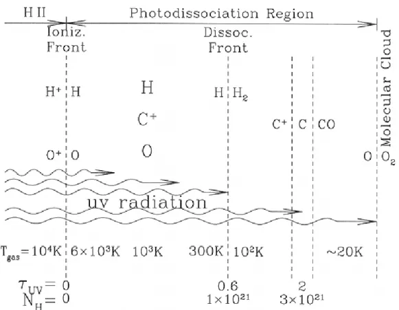
The warm surface of molecular clouds is called Photon-Dominated Region (PDR). This is a region where the chemical and physical conditions are dominated by the local photon density. FUV-photons with energies be- tween 6 eV and 13.6 eV, provided by hot and young stars (O, B and Wolf- Rayet stars) or by the ambient interstellar radiation field (ISRF), play an im- portant role in the thermal and chemical balance of interstellar gas (Hollen- bach & Tielens, 1999). In PDRs, different heating and cooling processes are present e.g., photo-electric emissions from dust grains and cooling by fine-structure emissions of [CII], and [OI] (Kaufman et al., 1999; Röllig et al., 2007; Sternberg & Dalgarno, 1995). PDRs contain layered struc- ture because interstellar dust shields species from FUV-photons, hence chemical stratifications are produced by the progressively weaker FUV- field (Ossenkopf et al., 2007).

A schematic representation of a PDR is shown in Fig. 2.1. The surface part of a PDR (relative to the position of the UV radiation source) has a thin transient region in which most species are ionized, and is called ionization front. Behind this front, the ionized atoms become neutral and the FUV-photons can penetrate into the cloud. Thus, there is still strong enough radiation (therefore high temperature and strong heating) to be able to dissociate hydrogen. The FUV radiation is absorbed by dust grains and PAHs (Polycyclic Aromatic Hydrocarbons). The absorption energy is used to heat the grains and excite PAHs. This part of a PDR emits contin- uum emission in FIR and the PAH lines in infrared wavelengths (Bakes &

Tielens, 1994; Weingartner & Draine, 2001). The gas is heated by photo-

electrons (Section 2.5.1) which heat the neutral gas (Tielens & Hollenbach,

2.5 Photon-Dominated Regions (PDRs) 19

Figure 2.1: A schematic figure about the structure of a PDR (Draine, 2011).

1985; Watson, 1972; Wolfire et al., 1995). Deeper in PDRs another thin region exists, it is called dissociation front. In this front, the molecular hy- drogen (H

) starts to be dominant rather than atomic hydrogen (H). Slightly deeper in the cloud, ionized carbon recombines to produce atomic carbon and

CO.

2.5.1 Energy balance

Heating

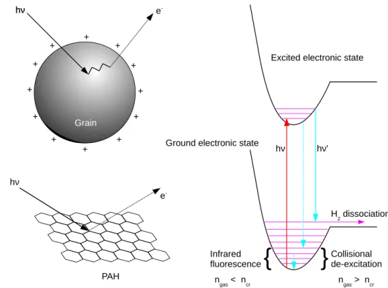
Photoelectric heating on grains and PAHs The photoelectric heating

(PE-heating, hereafter) process is the dominant heating process in the

ISM (Fig. 2.2). In this process, an electron can be ejected from the grain

surface when an FUV-photon collides with a dust grain. The kinetic energy

of the electron heats up the ambient gas. The efficiency of PE-heating is

reduced for highly ionized grains. If the FUV radiation field is attenuated,

and the grains are mainly neutral, the PE-heating is more efficient.

+ + +

+ + +

+

+ +

+ +

+

e^- hν

Grain hν

PAH hν

e^-

hν hν'

{ }

de-excitation Infrared

fluorescence

n_gas < n_cr n_gas > n_cr Excited electronic state

Ground electronic state

H₂ dissociation

Figure 2.2: A basic figure on how the photoelectric heating works on dust grains and PAHs (left panel) and a schematic diagram of the photo- pumping of H

(right panel).

Photo-pumping of H

In this case, an absorbed FUV-photon electron- ically excites H

which decays back to an excited vibrational level in the ground electronic state (or if the gas density is low enough [n < n

∼ 10

cm

, (Martin & Mandy, 1995; Martin et al., 1996)] to the ground vibra- tional state producing infrared emission, Fig. 2.2). If the gas density is large (n > n

∼ 10

cm

) another de–excitation mechanism becomes important which is responsible for the gas heating, namely collisions with hydrogen.

Nevertheless, it is also possible that the photon fluoresces back to the vibrational continuum level in the ground electronic state. In that case, the molecular hydrogen is destroyed by photo-dissociation. If the molec- ular hydrogen column density is large enough, which means optically thick lines, all of those photons are absorbed by H

in the outer part of the molecular cloud that could cause UV fluorescence photo-dissociation.

This effect is the so–called self–shielding of H

. Because the rate of photo-

dissociation of molecular hydrogen depends on the column density, the

H/H

transient region is very thin and sharp.

2.5 Photon-Dominated Regions (PDRs) 21 Dust–gas heating Usually the dust and gas do not have the same tem- perature (T

6= T

), and are not in thermodynamic equilibrium

. If T

> T

, the gas atoms leap from the grain surface and put energy into the dust environment, thus the gas can be heated up. On the other hand, if T

< T

(in, for example, PDRs or the diffuse ISM), this pro- cess becomes a gas cooling mechanism.

Cosmic–ray heating It is a dominant source of gas heating at the dense part of PDRs, far from the ionization front, where the ambient FUV radi- ation field is almost completely attenuated. In a localized place in the interstellar medium, where high cosmic–ray ionization occurs, cosmic rays with low energy [∼ 100 MeV, (Tielens, 2005)] could play a dominant role in gas heating

.

Cooling

The photo-dissociation regions are mainly cooled by emission of collision- ally excited far–infrared fine-structure lines [e.g., [OI] at λ = 63 µm and λ = 146 µm, [CII] at λ = 158 µm which are also useful as a diagnostic tool for the temperatures and densities of emitting regions (Liseau et al., 2006)] and by rotational transition lines (e.g.,

CO, OH, H

O). The relative dominance of these lines depends on the chemical composition of the gas phase (Tielens & Hollenbach, 1985) and physical parameters such as the density. For example, in a low density region [n n

([CII]) ∼ 3 × 10

cm

, (Mookerjea et al., 2011)] [CII] emission dominates the cooling (Abel et al., 2005; Abel, 2006; Heiles, 1994; Kaufman et al., 2006). On the other hand, [OI] (

P

→

P

) is an important cooling line at high densities [be- cause this line has a high critical density n

≈ 5 × 10

cm

, (Mookerjea et al., 2011; Röllig et al., 2006)]. Additionally, PDRs could be cooled by col- lisionally excited infrared ro-vibrational lines of molecular hydrogen. Also, if the density is high enough, then another cooling process becomes im- portant, namely the collisions with cooler dust grains (Burke & Hollenbach, 1983).

5

In dark clouds, where no UV photons are entering, and under high density conditions dust and gas are in equilibrium.

6

There are another heating mechanisms which could be important under certain cir-

cumstances (e.g., photo-dissociation of H

, photo-ionization of C, X-ray heating, turbulent

and shock heating, gravitational heating.)

2.6 Chemistry in the ISM

The interstellar chemistry was impelled by the discoveries of atoms, ions and molecules in the ISM

. In the ISM, two kinds of chemistry can be dis- tinguished: gas–phase and grain–surface chemistry. The chemical reac- tions are (mainly) governed by photons, electrons and collisions of differ- ent types of molecules and atoms. To be able to model the observations, different models have been developed which take into consideration the simplified geometry of a cloud (spherical or plan-parallel approach) and the main chemical reaction types in both gas-phase and grain–surface chemistry. I introduce only the important chemical reaction types because a short description of the models that I applied will be described in Chapter 7.

2.6.1 Gas phase chemistry

Photodissociation: AB + hν −→ A + B. The chemistry in PDRs is mainly driven by FUV photons which can destroy the molecules (dissociate them).

This procedure is important if the molecular cloud is located in the vicinity of OB stars.

Neutral–neutral: A + B −→ C + D. Another important reaction type is the neutral–neutral chemical reaction which is relatively slow. It is because this reaction needs additional energy to overcome the activation barrier of the neutral species.

Ion–neutral: A

+ B −→ C

+ D. Because the reactant is an ion, which means higher energetic state, these reactions have no activation barrier, or at least it is very low, therefore this reaction can be faster at low temper- atures than neutral–neutral reaction.

Dissociative electron recombination: A

+ e

−→ C + D. This type

of reaction could be important in those parts of clouds where the electron

density is high enough (for example, at or close to the ionization front in

PDRs).

2.6 Chemistry in the ISM 23

Accreation

Diffusion

Reaction

Ejection

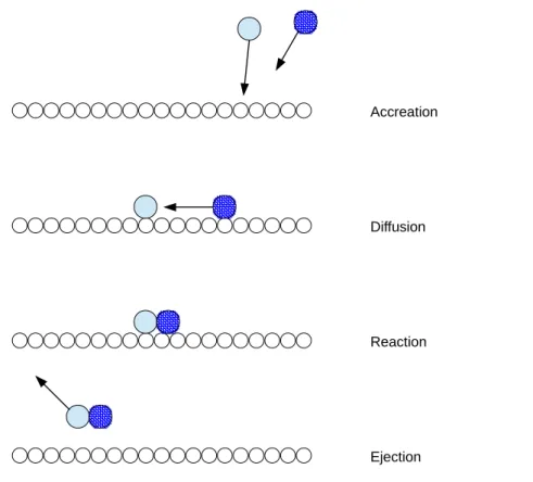
Figure 2.3: A schematic figure on the possible reaction types of two species on grain surface (Tielens, 2005).

2.6.2 Grain surface chemistry

Even if the chemistry and the chemical structure of a molecular cloud mainly depends on the abundance of hydrogen and the gas–phase heavy elements (Sternberg & Dalgarno, 1995), the dust grains play an important role in chemistry as well. The time scale for a process on the grain sur- face is set by the accretion rate. The accretion rates can be expressed as (Tielens, 2005):

k

= vσ

n

S(T, T

) (2.25) where v is the velocity of species, σ

is the grain cross section, n

is the density of grains, and S(T, T

) is the sticking coefficient which depends on the temperature of gas and dust. The surface atom which is bonded to the surface only by a weak van der Waals force is physically adsorbed (physisorbed). Because of this weak bond, that kind of surface atoms have a high mobility on the surface. On the other hand, it is possible for

7

Nowadays, around 200 species have been detected in the interstellar medium (see,

for example, at http://www.astro.uni-koeln.de/cdms/molecules).

some species to stick to the grain surface with much stronger bond. This is called chemisorbtion because the bonding to the grain surface is a strong covalent bond. Therefore, chemisorbed species have a very low mobility and they cannot easily move on the surface

. The mobility is an important

“parameter”. If there are two species with high mobility (which means they have high probability to meet each other) on the grain surface, then the reactions between these species are driven mainly by collisions. This is called Langmuir–Hinshelwood mechanism. Another mechanism, called Eley–Rideal mechanism, occurs when a gas–phase element hits directly an unmobile atom on the grain surface.

The temperature of the dust grain is also important because, if it is high enough, only chemisorbtion is relevant, because the probability of the evaporation of physisorbed atoms increases with the dust temperature.

8

The chemisorbed hydrogen moves on the grain surface via a quantum tunnelling ef-

fect, while species heavier than hydrogen can only move on the grain surface via thermal

hopping.

3

Observations by the Herschel Space Observatory

In this chapter, I give a brief description about the space mission Herschel Space Observatory (Section 3.1). After that, I shortly describe which in- struments we used for taking scientific data (Sections 3.1.1 and 3.1.2), what kind of observing modes are possible, and which of them were used by us (Sections 3.1.1 and 3.1.2). The data I present in the thesis are part of the WADI–program (Section 3.2) and the one of target sources of this key–project was NGC 3603 (Section 3.2.1).

3.1 The Herschel Space Observatory

The Herschel Space Observatory [(Pilbratt et al., 2010), hereafter Her-

schel], has the largest single mirror in space so far and carried three instru-

ments [Photodetector Array Camera and Spectrometer (PACS), (Poglitsch

et al., 2010); Heterodyne Instrument for the Far Infrared (HIFI), (de

Graauw et al., 2010) and Spectral and Photometric Imaging REceiver

(SPIRE) (Griffin et al., 2010)] covering a spectral range from the FIR to

sub–millimetre (submm). Because molecule rotational transitions are in

the submm and FIR regimes and most of the desired species are observed

by the instruments HIFI and PACS, I shall give a short introduction of these

instruments. On the other hand, I also investigated the combination of

SPIRE and PACS data (using SPIRE PACS Parallel Observing Mode) to

study the dust and UV field distribution (Section 5.3). Therefore, I give a

very short introduction about SPIRE, too (Section 3.1.3).

Table 3.1: The main parameters of the Herschel Space Observatory

S/C type: Three-axis stabilised

Operation: 3 hrs ground contact period/day

Dimensions: 7.5 m ×4.0 m (height × diameter)

Telescope diameter: 3.5 m

Total mass: 3170 kg

Solar array power: 1500 W

Average data rate to instruments: 130 kbps

Absolute pointing error: 2.45

(pointing)/2.54

(scanning) Relative pointing error: 0.24

(pointing)/0.88

(scanning) Spatial relative pointing error: 2.44

Cryogenic lifetime from launch: at least 3.5 years

3.1.1 HIFI

HIFI can be used for spectroscopy from high to very high spectral resolu- tion (1 − 0.125 MHz) in a wavelength range of ∼ 625 − 240 (480 − 1250 GHz) and 213 − 157 (1410 − 1910 GHz) µm. These ranges are split into 7 mixer bands each with vertical and horizontal polarizations. HIFI has four spec- trometers: two Wide Band Acousto–Optical Spectrometers (WBS) and two High Resolution Autocorrelation Spectrometers (HRS) that can be used in both polarizations. HIFI uses heterodyne technique

which means the signal from the sky (ν

) is mixed with a signal from a local oscillator (ν

). The intermediate frequency (ν

) is the difference of the sky and LO frequencies: ν

= ν

− ν

. Because HIFI works as a double side- band (DSB) receiver both signals [ν

+ ν

(upper sideband, USB) and ν

− ν

(lower sideband, LSB)] are detected at the same time (Roelf- sema et al., 2012).

Observing modes with HIFI

Basically, four kinds of observations are possible with HIFI: position, dual beam and frequency switch, and load chop. The selection of the observing modes depends on, for example, the properties of a target source (e.g.

how extended the source is). The possible observing modes with HIFI are:

1. Single point: with one position on the sky

1

Many books can give more detailed description about the different heterodyne tech-

niques, e.g. Hall et al. (1981); Kroger (1967); Menzies (1976); Nahin (2001); Schultz

(2004) and Wadley (1959).

3.1 The Herschel Space Observatory 27

• Position switch (PS)

• Dual beam switch (DBS)

• Frequency switch (FS)

• Load chop (LC)

2. Maps: to observe extended sources

• On-the-fly (OTF) with position switch

• OTF with frequency switch

• Raster with dual beam switch

3. Spectral scans: for line surveys with one position on the sky

• Dual beam switch

• Frequency switch

• Load chop

We received single point observations with dual beam switch mode and OTF maps, thus I give a short description about these observational meth- ods.

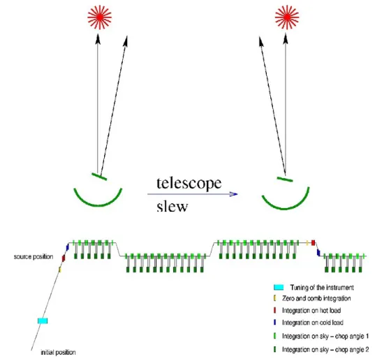
DBS, single point observation. In this case, the beam is moved by the secondary (or internal) mirror between the ON and OFF reference posi- tions. For OFF measurements, if it is possible, we observe the blank sky with no emission to correct the observed spectra for the background sky noise and for calibration of the instrument itself. This method is efficient be- cause the OFF position is relatively close to the ON position (< 3

), hence the telescope and internal mirror movements are short which increases the efficiency of the observation (more time on source). Also, because of the small motions of the telescope and the secondary mirror (Fig. 3.1), this observing method provides good quality data without standing waves due to the dual chop motions. Because the chopper mirror changes the path of the incoming light, some standing wave could still exist. But if we have the source on both ON and OFF positions (due to the telescope movement) the standing waves can be eliminated or minimized. This leads to stable baselines and good intensity calibration.

On-the-fly (OTF) map. This is the most time efficient observing method

with HIFI (basically, the total time of the observing time can be used on

the source). The telescope scans the source in rows and every second

row has an opposite scan direction (Fig. 3.2). During the scans, there

are data readouts at regular time intervals. The default time interval of the

readouts is Nyquist-sampled. It means, that the data readouts places at

shorter scanning distance than half beam size (HFBS) at the observational

frequency. For example, the sampling sizes in case of band 1a is 18 .

4 for

Figure 3.1: Top: The light paths from the source. Bottom: schematic figure on the dual beam switch observing mode (Jackson et al., 2007).

Figure 3.2: Schematic figure on the on–the–fly observing mode. The green dots show the readouts (Jackson et al., 2007).

Nyquist– and is 22

for half–beam sampling (Schieder, 2010). This leads

to no loss of spatial information and data with no aliasing. After a certain

period, OFF measurements are also included for blank sky subtraction.

3.1 The Herschel Space Observatory 29

3.1.2 PACS

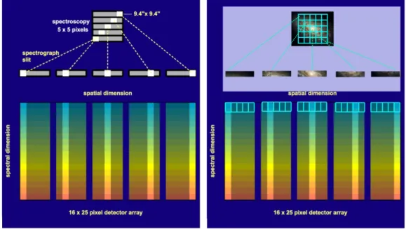
The PACS instrument has two modes: imaging dual-band photometry and integral-field spectroscopy (Poglitsch et al., 2010). To be able to investi- gate the different transitions of important cooling lines, we used PACS due to its capability to observe at shorter wavelengths than HIFI ( . 157 µm).

Because we only used the spectroscopy part, I give a more detailed de- scription of the spectrometer.

The spectrometer has a wavelength range of 51 µm to 220 µm which is divided into two channels: blue (51 − 105 µm) and red (102 − 220 µm). The spectrometer also has different “units”: the basic unit of detector is called as a pixel, and a module which has 16 pixels in 25 columns. The total field of view (FOV) is 47

× 47

which is assured by 5 × 5 spatial pixels (spaxels). The spaxels are the basic unit of the integral field of PACS.

The individual spaxels cover an area of 9 .

4 × 9 .

4. Figure 3.3 shows how the spaxels cover the given observed field and how the image slicer does work: it redistributes the 2D FOV into 1 × 25 slices as shown in Fig. 3.3.

The advantage of the combination of the spectral and spatial resolutions is the efficiency of the observation of weak lines. The real footprint of the spaxels on the sky can be seen on Fig. 3.4. The real distribution of the spaxels depends on the position angle of the pointing. In cases of nod A and B, there is also a small shift (∼ 2

) between each spaxel because of the optical distortions between the chopper ON and OFF positions.

Figure 3.3: How the integral-field spectrometer works: each spaxel is

projected into the detector arrays Altieri & Vavrek (2011).

Observing modes with PACS

There are two main observing modes:

1. Line spectroscopy

• Chopping/nodding spectroscopy

• Unchopped grating scan 2. Range spectroscopy

• Chopping/nodding spectroscopy

• Unchopped grating scan

We used line spectroscopy with chop/nod mode and range spectroscopy with unchopped grating scan mode. Thus, a short description about these observing modes will be given.

Line spectroscopy with chop/nod mode. This observing technique is ideal for faint lines with faint or bright continuum. We can select the combination of the wavelength range in which we want to observe: first (102− 210 µm) and second (71− 105 µm) order, or first and third (51−73 µm) order. This is available for range spectroscopy, too. It is also possible to change the chopper throw between 1.5

, 3

or 6

(“small”, “medium” and

“large”, respectively). These values correspond to the rotation of the foot- print on the source observation (in both nod positions). In the example shown on Fig. 3.4, the observing sequence is going from the top left (green signs → nod A–OFF) to the bottom right (purple signs → nod B–OFF). In this case, we had one nod cycle which means the whole nod sequence looks like A-A-B-B: nod A–OFF → nod A–ON → nod B–ON → nod B–OFF.

Such a sequence can be repeated, if needed, to observe fainter lines.

Range spectroscopy with unchopped grating scan. In this mode, the observations of one line or several line features are possible, too, like in case of line spectroscopy. This mode allows the observers to define a wavelength range or the full range (SED mode). The other similarity with line spectroscopy is the different chopper throws (except in map mode where only one throw is available, namely the “large”). The unchopped grating scan can be done with Nyquist-sampling or with high-sampling density.

3.1.3 SPIRE

This instrument has an imaging Fourier–transform spectrometer (FTS) and

a three–band imaging photometer. The photometer (which provides a

3.1 The Herschel Space Observatory 31

Figure 3.4: An example of the real footprints on the sky. Left plot: the PACS footprints (ON and OFF positions are included) and the Herschel boresight (grey crosses). The red square indicates the position of the source. The green and purple crosses mark the OFF positions (nod A and nod B, respectively), while the red and blue crosses show the ON position (nod A + nod B). Right plot: the enlargement of the ON position which shows the real footprint on the sky. The red circles show the sequence direction of the numbering of the spaxels: the top right-most represents the 0, 0 spaxel, then, as we go down, 0, 1 and 0, 2 etc. The left-most at the bottom is the 4, 4 spaxel.

broad–band photometry with λ/∆λ ∼ 3) uses three bands with approxi- mate center wavelengths of 250, 350 and 500 µm. These bands are called PSW, PMW and PLW respectively and have different layout of photometer arrays [more detailed descriptions about SPIRE can be found in, for exam- ple, Griffin et al. (2010)]. To investigate the distribution of dust and UV field strength in NGC 3603, I used a Level–2

public photometry data set from SPIRE PACS parallel observing mode

. The observational ID I used was 1342203064 which is a line scan with fast scan speed (60

/s) and covers a large map (120

× 120

) about the surrounding area of NGC 3603. On the other hand, I focused only on a very small fraction of the whole map which is included NGC 3603.

2

More information about SPIRE pipeline steps can be found at http://herschel.

esac.esa.int/twiki/bin/view/Public/SpireCalibrationWeb?template=viewprint

3

http://herschel.esac.esa.int/Docs/PMODE/html/parallel_om.html

3.2 The WADI key–project

The physical and chemical processes in molecular clouds are strongly in- terconnected; the density and temperature of interstellar material define the possible chemical reactions. The surroundings of young and massive stars are heavily influenced by UV radiation emitted by these stars and that radiation and possibly strong stellar winds govern the local physical, and chemical conditions.

The Herschel guaranteed time key–project “The Warm And Dense ISM”

[WADI, PI: PD. Dr. Volker Ossenkopf, (Ossenkopf et al., 2010a, 2011)] in- vestigated these interactions via observations of different molecular clouds (concentrating on the thin interaction zones, the so–called PDRs; Section 2.5). The observations are focused on three basic scientific topics, namely the chemistry, dynamics and energy balance of molecular clouds, e.g., what kind of physical processes and conditions can trigger star formation in molecular clouds?; how the UV radiation field interacts with molecu- lar clouds (and/or how the strong stellar wind, provided by hot and young massive stars, influences the interstellar gas in their environment)? The key-project is also interested about the chemistry: which reactions domi- nate and could lead to the formation of more complex molecules?

Observing light hydrides (e.g., CH, NH etc.) and deriving column den- sities can help to improve chemical models. Also, the observed carbon species (

CO,

CO,

C

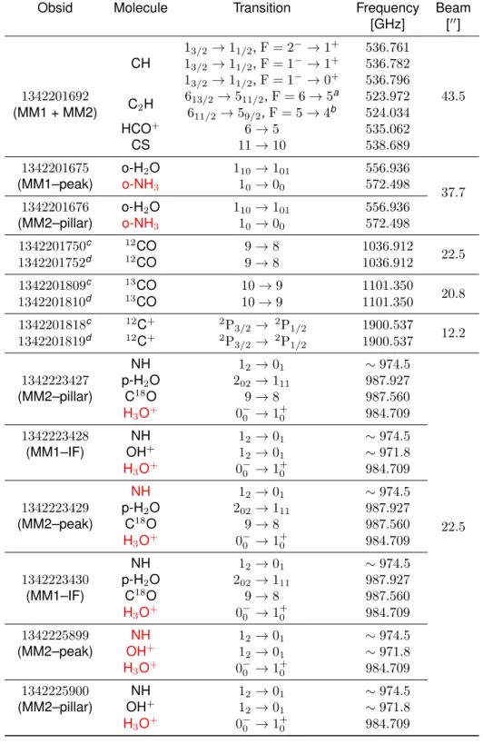
) could allow us to determine abundance ra- tios that can lead to a better understanding of carbon fractionation which is still not clear. Because Herschel has a very good velocity resolution, the investigation of detected emission lines can help to study the velocity structures of an observed molecular cloud. Investigation of the physics of energy balance can be done, for example, by comparison of cooling line intensities ([OI], [CII]). In this thesis, I shall concentrate the center part of a molecular cloud complex and shortly describe it in Section 3.2.1 then give summaries of the observations (Tab. 3.2 and 3.3, and Appendices A and B).

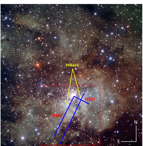
3.2.1 The target source: NGC 3603

With a total bolometric luminosity of L

> 10

L (Stolte et al., 2004), NGC 3603 is 100 times more luminous than the Orion Nebula and one of the most prominent HII regions in our Galaxy. It is located in the Carina spiral arm (the coordinates

of NGC 3603 are: α

= 11

15

09 .

1 and δ

= −61

16

17

) with a distance of about 7−8 kpc (Melena et al., 2008), and a total gas mass of ∼ 4 × 10

M (Grabelsky et al., 1988). It has

4

From SIMBAD: http://cdsweb.u-strasbg.fr/