on quantitative traits
Inaugural-Dissertation zur
Erlangung des Doktorgrades
der Mathematisch-Naturwissenschaftlichen Fakult¨at der Universit¨at zu K¨oln
vorgelegt von
Nico Riedel
aus Mettmann
K¨oln 2016
Prof. Dr. Michael L¨assig
Tag der m¨undlichen Pr¨ufung: 28.06.2016
The concept of evolution, which was introduced by Charles Darwin in 1859, and also its mathematical description by the theory of population genetics are well-established.
Population genetics describes the development of a population under the influence of mutations, creating new genetic variants, and natural selection, increasing the fre- quency of favorable phenotypes. Yet, the experimental verification of selective forces acting on species has proven difficult. With new experimental techniques that have been established in the field of quantitative genetics, like the sequencing of DNA or measurements of gene expression levels, it has become possible to find signs of natural selection on the level of the genome.
In this thesis, I develop a statistical test based on population genetics theory that can infer lineage-specific differences in selection between multiple lines of a species.
The test employs data from quantitative trait experiments and uses a log-likelihood scoring to quantify the evidence for different selective scenarios. I show that the use of multiple lines increases both the power and the scope of selection inference. Extensive numerical simulations demonstrate that the test can distinguish selection from neutral evolution as well as different scenarios of lineage-specific evolution. The principle of maximum entropy is used to derive a modified version of the selection test that accounts for the multiple testing problem arising when many traits are tested for selection at the same time. The developed test is applied to two published plant datasets and a published dataset of gene expression levels in three yeast lines. In all cases, I find signs of selection not seen with a two-line test. For the yeast dataset I find pervasive adaptation linked to stress resistance both on the level of individual genes as well as for larger gene modules consisting of several genes, like protein complexes and pathways.
This adaptation signal is also reflected on the protein levels.
Sowohl das Konzept der Evolution, welches 1859 von Charles Darwin eingef¨uhrt wurde, als auch die mathematische Beschreibung durch die Populationsgenetik sind seit langem etabliert. Die Populationsgenetik beschreibt die Entwicklung einer Population unter dem Einfluss von Mutationen, welche neue genetische Varianten erzeugen, und der nat¨urlichen Selektion, welche die H¨aufigkeit der g¨unstigen Phenotypen erh¨oht. Jedoch hat es sich als schwierig erwiesen, diese selektiven Kr¨afte experimentell nachzuweisen.
Neue experimentelle Techniken die sich im Feld der quantitativen Genetik etabliert haben, wie das Sequenzieren der DNA oder der Messung von Genexpressionsleveln, haben es erm¨oglicht, Spuren der nat¨urlichen Selektion auf dem Level des Genoms nachzuweisen.
In dieser Dissertation entwickle ich einen statistischen Test welcher auf der Theorie der Populationsgenetik basiert und mit welchem man linienspezifische Unterschiede in der Selektion zwischen verschiedenen Linien einer Spezies nachweisen kann. Dieser Test verwendet Resultate von Experimenten ¨uber quantitative Merkmale und ver- wendet einen Log-Likelihood-Quotienten um die Evidenz f¨ur verschiedene selektive Szenarien zu quantifizieren. Ich weise nach, dass die Verwendung von mehreren Lin- ien sowohl die Leistungsf¨ahigkeit als auch den Anwendungsbereich des Selektionstests vergr¨oßert. Umfangreiche numerische Simulationen zeigen, dass der Test zwischen Selektion und neutraler Evolution als auch zwischen verschiedenen linienspezifischen Evolutionsszenarien unterscheiden kann. Das Prinzip der maximalen Entropie wird verwendet um eine modifizierte Version des Selektionstests herzuleiten, welche das multiple Testproblem ber¨ucksichtigt, welches auftritt, wenn viele Merkmale gleichzeitig auf Selektion getestet werden. Der entwickelte Test wird auf zwei publizierte Pflanzen- datens¨atze sowie einen publizierten Datensatz zu Genexpressionsleveln in drei Hefe- linien angewandt. In allen F¨allen finde ich Hinweise f¨ur Selektion, welche nicht durch einen Zwei-Linien-Test entdeckt werden. F¨ur den Hefedatensatz finde ich weit verbre- itete selektive Anpassung die mit Stressresistenz verbunden ist, sowohl auf dem Level einzelner Gene als auch f¨ur gr¨oßere Genmodule, die aus mehreren Genen bestehen, wie zum Beispiel Proteinkomplexen. Diese Adaption kann auch f¨ur die Proteinlevel nachgewiesen werden.
1 Introduction 9
2 Genetics and evolution 11
2.1 The Genome . . . . 12
2.1.1 DNA . . . . 12
2.1.2 Genes and proteins . . . . 12
2.2 Quantitative traits and QTL mapping . . . . 13
2.2.1 Quantitative traits . . . . 13
2.2.2 QTL mapping . . . . 13
2.3 Population genetics and evolution . . . . 16
2.4 Connection to statistical physics . . . . 18
3 Multiple-line selection model 21 3.1 Idea of the selection test . . . . 21
3.2 Derivation of the model . . . . 22
3.3 Inference of selection and log-likelihood scoring of evolutionary scenarios 28 3.4 Advantages of multiple-line testing . . . . 31
3.4.1 Increase in the number of detected loci . . . . 31
3.4.2 Two vs. three lines at a constant number of crosses . . . . 35
3.5 Statistical power of the selection test . . . . 38
3.6 Robustness of the model assumptions . . . . 40
3.6.1 Epistasis and multiple segregating loci . . . . 40
3.6.2 Evolutionary timescales . . . . 45
3.7 Comparison to other selection tests . . . . 46
4 Multiple Testing and Maximum Entropy 49 4.1 Classical multiple testing corrections . . . . 50
4.1.1 Holm-Bonferroni Correction . . . . 50
4.1.2 Benjamini–Hochberg procedure . . . . 50
4.2 Conditioning on the trait difference . . . . 51
4.2.1 Pedagogical example . . . . 52
4.2.2 Derivation of the ascertained neutral scenario . . . . 55
5 Short evolutionary times 63 5.1 Two lines . . . . 63
5.2 Three lines . . . . 66
5.3 Statistical power of the short-time test . . . . 69
6 Selection on Plant Quantitative Traits 71 6.1 Maize photoperiodic response traits . . . . 71
6.2 Mimulus floral traits . . . . 74
7 Gene expression evolution in the yeast S. pombe 79 7.1 Yeast dataset . . . . 80
7.1.1 Available data . . . . 80
7.1.2 State configurations . . . . 81
7.2 Selection on individual genes . . . . 84
7.2.1 State configurations per gene . . . . 84
7.2.2 Selection analysis . . . . 86
7.2.3 Multiple testing correction . . . . 89
7.2.4 Adjusting for the high QTL false discovery rate . . . . 89
7.2.5 Lines with highest trait divergence . . . . 91
7.2.6 Pleiotropy . . . . 93
7.3 Selection on gene modules . . . . 96
7.3.1 State configurations per gene module . . . . 96
7.3.2 Selection analysis . . . . 97
7.3.3 Stress-specific gene modules under selection . . . . 99
7.3.4 Biological functions of gene modules under selection . . . 101
7.4 Protein level changes . . . 107
7.5 Possible use of protein QTL data . . . 109
7.6 Comparison to other selection tests . . . 110
7.6.1 Orr test . . . 110
7.6.2 Test for genome-wide level of selection . . . 111
8 Conclusions 113
Appendix 114
Introduction
In the past decades the field of quantitative genetics has experienced a tremendous progress. Quantitative genetics deals with traits of an organism that vary continuously (called quantitative traits), like the height of a plant or the expression level of a gene, and their underlying genetic basis. The development of the method of QTL analysis allowed to map observed changes in the phenotype, like changes in morphology, to the genome. This method helped to uncover the genetic basis of quantitative traits (Mackay 2004; Mackay et al. 2009). In numerous organisms like crop, cattle, or yeast genetic loci underlying many traits have been determined (Marullo et al. 2007; Goddard and Hayes 2009). In recent years, new, advanced experimental techniques have allowed the mapping of all gene expression or protein levels of an organism simultaneously, taking quantitative trait analysis from a level of individual macroscopic phenotypes to the level of changes in genes underlying these phenotypes (Hoheisel 2006; Bantscheff et al. 2007).
Furthermore, crossing multiple lines has allowed to study a greater genetic diversity underlying many quantitative traits. Yet, many challenges still persist. Identifying the genes underlying quantitative trait loci has proven difficult and was only possible with further experimental effort for individual cases (Fanara et al. 2002; De Luca et al.
2003) and interactions between different genetic loci have also complicated the picture of the genetic architecture underlying quantitative traits.
On the theoretical side, the field of population genetics has been long established, building the theoretical foundation for the stochastic evolution of populations under the influence of natural selection, mutations and random fluctuations in the composition of the population (called genetic drift) (Hartl et al. 1997). The theory of population genetics uses stochastic differential equations to describe the time evolution of a pop- ulation which allows to gain insights into the dynamics of the evolutionary process.
Established results describe the probability for new, beneficial mutations to spread in a population as well as the time it takes to fixation. There is also an close connection between the fields of population genetics and statistical physics (de Vladar and Bar-
ton 2011b). The time evolution of allele frequencies in a population can be described using stochastic differential equations and the steady state of a population, balancing the forces of selection (increasing the fitness) and random genetic drift (decreasing the fitness), can be determined using methods of statistical mechanics.
In this thesis, I combine aspects of both fields to study the evolutionary history of quantitative traits. Based on established results from population genetics theory I construct a model for the evolution of quantitative traits. This model quantifies the strength of evidence for selection acting on a particular trait. I define a log-likelihood score that weights different selective scenarios against each other. The model is defined for an arbitrary number of lines and I show that using multiple lines increases both the power and the scope of selection inference. First, a test based on three or more lines detects selection with strongly increased statistical significance. Second, a multiple- line test allows to distinguish different lineage-specific selection scenarios, unlike in the case of two lines. Extensive numerical simulations show the ability of the test to distinguish neutral evolution from selection as well as different scenarios of lineage- specific selection. I show explicitly how the sensitivity of the test depends on the number of lines. Different violations of the model assumptions, like epistasis or shorter evolutionary timescales, are investigated, showing the overall robustness of the model.
In addition to the case of long evolutionary times considered in the original model, I also give a solution for short evolutionary times. The multiple testing problem that arises when many traits are tested for selection is considered. Using the principle of maximum entropy, I derive a modified version of the developed selection test that accounts for a possible ascertainment bias.
I apply the multiple-line test to QTL data on floral character traits in plant species of the Mimulus genus and on photoperiodic traits in different maize lines, where sig- natures of lineage-specific selection are found that are not seen in a two-line test.
Finally, I use a dataset of expression QTL (eQTL) for three lines of the yeast species Schizosaccharomyces pombe to study the adaptation of oxidative stress response both for individual genes as well as for gene modules, like protein complexes or pathways. I consistently find high levels of selection on both genes and gene modules. The analysis of gene modules exclusively under selection in the stress condition uncovers the adap- tation of stress response on the level of individual genes and protein complexes. An analysis of the protein levels connected to the expression levels shows that the selection on the transcriptional level is also reflected in translational changes.
Genetics and evolution
The field of genetics has undergone a rapid development during the last decades. Build- ing upon the success of the discovery of DNA as the carrier of the genetic information necessary for the functioning and reproduction of an organism, the understanding of the structure and functionality of the genome has progressed. Many new experimental techniques changed genetics into a quantitative field (Hoheisel 2006; Bantscheff et al.
2007). Nowadays it is possible to measure the genetic sequence of numerous organisms, including humans (Metzker 2010). The field of quantitative genetics contains a rich variety of interesting mathematical problems and challenges connected to statistical physics. For example, the evolution of species is a stochastic system. Many processes inside organisms like the activity and regulation of genes and its time dynamics is a many-body problem with strong interaction between the individual elements of the system. Numerous inference problems appear in this context, where the result of a process is observed (like in the evolution of species), while the underlying dynamics are unknown. The contribution of statistical physics is to build appropriate mathemat- ical descriptions of the underlying processes which for example allow to infer model parameters from experimental observations.
In this chapter I introduce the basic genetic concepts necessary to understand the background and motivation for the selection test developed in this thesis. I start with a short introduction to DNA and the genome. The notion of quantitative traits and quantitative trait loci (QTL) is explained, which are key concepts used for the selec- tion test. I end the introductory chapter with the topics of evolution and population genetics, which puts the evolution of a population in a quantitative context described by stochastic differential equations.
2.1 The Genome
2.1.1 DNA
The DNA (deoxyribonucleic acid) stores all the inheritable information of an organism.
It is a linear molecule consisting of the four nucleotides cytosine (C), guanine (G), adenine (A), or thymine (T). It is structured as a double helix of two complementary strands of nucleotides with pairwise bonds between the nucleotides C and G as well as A and T. During reproduction the whole DNA of an organism is duplicated. The genome denotes the sum of all DNA present in an organism, which is often distributed on different chromosomes, that are separate DNA molecules. The sequence information contained in the genome is called the genotype of an organism and can be measured through DNA sequencing (Metzker 2010).
2.1.2 Genes and proteins
Genes are the central elements of the genome. Genes serve as the blueprint for proteins, which are biomolecules that perform a vast number of functions in an organism. The coding region of a gene is marked by a characteristic starting sequence, also called pro- moter, and is read off by a protein called polymerase. In the step called transcription, the polymerase synthesizes a single stranded RNA molecule with the complimentary nucleotide sequence. This messenger RNA (mRNA) is in turn read off by the ribosome, where three nucleotides are read off at a time, forming a codon. Each codon is assigned an amino acid (the smallest components of a protein), where different codons can map to the same amino acid. This map from nucleotide codons to amino acids is called the genetic code and is almost universal among all life forms (Crick et al. 1961). All codons are read off sequentially to produce a sequence of amino acids, which form the protein sequence of the underlying gene. This step is called translation. In summary, the conversion of genetic information starts with the DNA sequence of a gene and is mediated via the mRNA to form a protein as a final product. This process is also known as the central dogma of molecular biology (Crick et al. 1970). A gene can exist in different variants which are called alleles.
Not all genes are needed in an organism at all times or in all tissues. Therefore, a complex gene regulatory system exists that controls the gene expression (gene expres- sion denotes the amount of mRNA produced from a gene in the step of transcription).
An example for important elements of gene regulation are transcription factor binding sites, which are typically located within the promoter sequence close to the starting point of a gene. These sites can bind proteins, that are called transcription factors, which can modulate the binding probability of the polymerase which in turn modu- lates the gene expression levels. Many genes are coding for proteins that can alter the
expression of other genes. Thus, all genes are part of a complex regulatory network with many interactions between genes.
2.2 Quantitative traits and QTL mapping
2.2.1 Quantitative traits
While the genome provides all genetic information - the genotype - of an organism, the phenotype of an organism is the set of all observable characteristics or traits. These can be morphological traits like size or color but also more microscopic traits like the expression level of a gene or a protein level. The phenotype of an organism is a result of two main factors, the genotype and environmental factors. While the genotype provides the basic information for all features of an organism, environmental factors like nutrition, temperature, or the surrounding ecosystem can influence the phenotype as well. Understanding the genotype-phenotype map, which captures the relationship between the genotypes of an organism and its observed phenotypes, is one of the central problems of genetics (Doerge 2002; Mackay et al. 2009). While the complete genotype- phenotype map is still out of reach, the genetic basis of individual phenotypes, like e.g.
yield traits in maize (Xing and Zhang 2010), has already been uncovered.
Some traits have a very simple genetic basis, with only a single genetic locus af- fecting the trait and with only a few possible characteristics, see Figure 2.1 (A). These traits are called Mendelian traits, as the Mendelian inheritance patterns can directly be observed. An example for this is the flower color of pea plants, as originally discovered by Mendel (Mendel 1866).
In contrast to this, most traits have a complex genetic basis with many genetic regions influencing the trait (Mackay et al. 2009). The combined influence of these genetic loci leads to an effectively continuous scale of trait characteristics, see Fig- ure 2.1 (B). These traits are called quantitative traits. Examples for quantitative traits are flower size (Chen 2009), leaf number (Coles et al. 2010), or bristle number in flies (Mackay and Lyman 2005). Any genetic region that has an influence on a quan- titative trait is called a quantitative trait locus (QTL). QTL can be genes linked to the phenotype or regulatory elements that alter the expression of these genes. Often, a QTL might be caused by allelic variants such as single nucleotide polymorphisms (SNPs), where only changes in individual nucleotides occur, in coding as well as non- coding regions (Stam and Laurie 1996; Harbison et al. 2004; Jordan et al. 2006; Zheng et al. 2010).
Figure 2.1: Mendelian traits and quantitative traits. (A) Mendelian traits are only governed by a single genetic locus (marked by the dark bar) in the genome and can only take on few distinct and clearly defined characteristics. (B) Quantitative traits are affected by many genetic loci. Taken together the effects of these loci generate an approximately continuous spectrum of possible trait values.
2.2.2 QTL mapping
Understanding the complex genetic basis of quantitative traits is a key step towards the genotype-phenotype map and is important in many different contexts like the understanding of complex diseases in humans (Plomin et al. 2009). QTL analysis allows to identify the QTL underlying a quantitative trait by linking phenotypic variation to genetic markers. This is done by crossing individuals of different strains (also called lines) of a species. These might be different breeding lines for cattle or crops (Goddard and Hayes 2009; Xing and Zhang 2010) or different strains of wild yeast isolates that were collected in different environments (Marullo et al. 2007; Gerke et al. 2009). In the crossed individuals the two genomes of lines 1 and 2 recombine (which happens in the second offspring generation orF2 generation for diploid organisms that have a duplicate chromosome set) and the alleles of the lines get reshuffled. In these crosses the genome is a mixture of DNA stretches originating from line 1 and stretches originating from line 2 (see Figure 2.2 (B)).
For the crosses the trait values T of the quantitative trait (e.g. plant height mea- sured in cm) as well as the genotype in form of genetic markers are measured. The goal of QTL mapping is to find genetic markers which are correlated with the trait value, i.e. to find markers where the trait value is on average higher when the allele of that marker is inherited from line 1, compared to the crosses with the marker allele from line 2. The genetic markers need to differ between the lines and to be evenly distributed across the genome with a sufficient density. These markers can be for ex- ample single nucleotide polymorphisms (SNPs) (Wicks et al. 2001) or microsatellites (repetitive DNA elements) (Somers et al. 2004). With QTL mapping the QTL cannot
Figure 2.2: The principle of QTL mapping. (A) The goal of a QTL mapping experiment is to determine the genetic basis underlying trait differences ∆T between different lines of a species. (B) To achieve this goal, individuals of the lines are crossed. The genome of the offsprings (the F2 generation for diploid organisms) is a mixture of the genomes of the parental lines created by recombination events between the genomes. A certain number of markers (M1. . .M4) spread over the entire genome is measured in the offsprings to determine from which line they originate. (C) QTL mapping algorithms are used to determine which markers are correlated with the trait. If the trait value of the crosses is on average higher when a marker originates from line 1, it is likely that a QTL close to the marker is affecting the trait. This likelihood is quantified by the QTL mapping algorithm. Markers for which the likelihood is above a significance threshold (red areas) are in linkage with a QTL. Since the QTL cannot be measured directly but only by linkage to nearby markers, the QTL mapping does not reveal the exact gene or mutation causing the QTL, but allows to infer the number and effects of QTL affecting a trait.
be identified directly. Instead, the markers are in genetic linkage with nearby QTL due to the rare frequency of recombination events, as the whole genetic region around a marker gets inherited from the same line (Lynch et al. 1998). Thus, QTL mapping only identifies markers that are close to a QTL, but it does not unravel the nature of the QTL itself. As another restriction of QTL mapping only the genetic diversity present between the lines can be uncovered. Since all QTL that have the same allele in both lines also have that allele in all crosses, no difference of the trait effect can be observed between the lines for these QTL.
QTL mapping is a computationally nontrivial task. Many effects like interactions between QTL (called epistasis) (Wang et al. 1999), multiple testing problems (arising due to the high number of possible trait-marker pairs) (Doerge and Churchill 1996), or a limited number of recombination events lead to complications in the analysis.
There are many different QTL mapping algorithms employing different techniques like the interval mapping (Lander and Botstein 1989), composite interval mapping (Zeng 1994), or multiple trait mapping (Jiang and Zeng 1995; Kao et al. 1999). Up to today, quantitative traits of many organisms have been mapped, ranging from bristle numbers or wing shape in Drosophila to yield traits in rice (Dilda and Mackay 2002; Mackay 2004; Mezey et al. 2005; Mackay and Lyman 2005; Bernier et al. 2007; Flint and Mackay 2009; Xing and Zhang 2010). But only in few cases and with additional exper- imental effort it was possible to fine-map individual QTL, identifying the gene or even the nucleotide change responsible for the QTL (Pasyukova et al. 2000; Fanara et al.
2002; De Luca et al. 2003; Moehring and Mackay 2004; Harbison et al. 2004; Jordan et al. 2006). In recent years, QTL analysis has also been expanded onto multiple-line crosses, where crosses between all possible pairs of the lines or backcrosses to a com- mon line are performed. It has been shown that utilizing information from several lines drastically increases the power and accuracy of QTL identification (Rebai and Goffinet 2000; Steinhoff et al. 2011) and the genetic variability that can be accessed (Blanc et al. 2006).
2.3 Population genetics and evolution
Evolution describes the change of the genetic composition of a population over time.
These changes can occur on the species level, with the creation of new species, or on the molecular levels, with e.g. changes in gene expression levels. Random genetic mu- tations lead to a genetic diversity in a population by creating new genetic variants.
Natural selection acts on the level of different genetic variants of a population. Some of the genetic variants might have favorable phenotypes that have a greater reproduc- tive success than other phenotypes. Since the individuals with favorable phenotypes accumulate a larger number of offsprings over the generations, this often leads to the
prevalence of the favorable phenotype.
The fitness of an organism is the measure of its reproductive success and is defined as the average number of offsprings of an individual (Wrightian fitness; for subtleties between slightly different definitions of fitness see also (Orr 2009)). If the fitness of all variants in a population is the same, the population is evolving neutrally. In this case, new mutants can become prevalent in the population without any effect on the reproductive success, which is called random genetic drift.
Population genetics is the mathematical description of the evolutionary process at the population level (Hartl et al. 1997). Central to population genetics is the evolution of a population of N individuals under the effect of mutations, selection and repro- duction. The evolution of a population is a stochastic process that can be described by a stochastic differential equation. While selection is a directed process, increasing the fraction of the fittest individual in the population, reproductive fluctuations lead to undirected changes in the composition of the population. These stochastic fluctua- tions are larger for smaller population sizes and tend to zero for very large populations, leading to an effectively deterministic evolution of allele frequencies in the population.
Mutations introduce new genotypes in the population that can have different fitness values than the ancestral genotype.
In the simplest case, a population consisting of two genotypesaandbwith (Malthu- sian) fitness Fa and Fb, respectively, evolves under the action of selection and repro- ductive fluctuations as (L¨assig 2007)
d
dtNa/b(t) = Fa/bNa/b(t) +χa/b(t), (2.1) where the population size Na/b(t) of individuals with genotype a or b, respectively, evolves according to a simple exponential growth law with a growth rate Fa/b. χa/b(t) is a noise term that describes the reproductive fluctuations in the population. It is defined as a Gaussian random variable with mean hχa/b(t)i = 0 and variance hχa(t)χb(t)i=Na(t)δ(t−t0)δa,b that describes uncorrelated white noise. The evolution of the population fraction x(t) = Na/(Na+Nb) can be written in term of a Fokker- Planck equation that captures the time evolution of the probability distribution of the x(t):
∂
∂tP(x, t) = 1 2N
∂2
∂x2x(1−x)P(x, t)−∆Fa,b(t) ∂
∂xx(1−x)P(x, t), (2.2) where N is the total population size and ∆Fa,b(t) = Fa(t) − Fb(t) (Kimura 1962;
L¨assig 2007). Without mutations introducing new genotypes, the population eventually reaches the fix points x = 1 orx = 0. Atx= 1 the whole population is monomorphic and only consists of individuals of genotype a, called fixation of the genotype, while at x= 0 the genotype a is lost.
In this context there are many interesting questions arising: What is the probability of fixation of a newly introduced mutation? How does this fixation probability depend on the fitness of the mutant? What is the distribution of fitness values of new mutants?
What is the typical time to fixation? How do different mutations that arise at the same time interact with each other?
The fitness of new mutants depends on the fitness landscape the population is living in. A fitness landscape is a theoretical construct that maps every genotype onto a fitness value, where a population tends towards genotypes with the highest fitness (’fitness peaks’) (Orr 2005). As the genotype typically consists of many factors the fitness landscape is often very high-dimensional. A single mutation can have vastly different effects on fitness depending on the type of the fitness landscape. A fitness landscape can be smooth, with the fitness contributions of different parts of the genotype adding up linearly. Otherwise there can be interactions between different alleles, called epistasis, where for example a certain combination of alleles that individually have a positive effect on fitness, leads to a decrease in fitness. This can make the fitness landscape more ’rugged’, create multiple peaks, and make it more difficult for a population to reach the global fitness optimum (Whitlock et al. 1995).
When new mutations are allowed in the model, the fix points where the population becomes monomorphic are not the end of the dynamics. Instead, new mutations arise from time to time and either get fixed or are lost. For this, the weak mutation limit is typically assumed where the time for a new mutation to arise is much longer than the time to fixation. Otherwise multiple competing mutations can arise, leading to a more complicated dynamics which is known under the name of clonal interference (Gerrish and Lenski 1998). For a new mutation to become fixed in the population, it has to overcome the random reproductive fluctuations. When only a single individual with the new mutation is present at the beginning, it can easily go extinct even when the mutant has a higher fitness than the rest of the population. It can be shown that the substitution rate ua→b that describes the fixation of genotype b (after the genotype arises via a mutation) in a population with genotype a is (Kimura 1962)
ua→b =N µa→b
1−exp(−2∆Fab)
1−exp(−2N∆Fab), (2.3)
where µa→b is the mutation rate for creating genotype b from genotype a. This result will be used later for the population genetics model underlying my selection test.
2.4 Connection to statistical physics
Even though statistical physics does not directly relate to the topics of genetics and evo- lution many concepts of statistical physics can be transferred to these fields of research
and can help to deepen the mathematical understanding in many cases. As mentioned before, population genetics deals with the stochastic evolution of a population, well described by stochastic differential equations. Many-body problems arise at numerous levels of genetics and evolution, as in the context of gene regulatory networks, with many genes that alter the expression of other genes, or at the level of species, with different species competing for limited resources in an environment. Evolution takes place on timescales that often span millions or billions of years, but only the species and genomes present today can be observed. This leads to many inference problems:
given the genomes of todays species, what is the evolutionary history of the lines and how are the species related? One of the great success stories was the inference of the famous tree of life, which describes the evolutionary relations of all species, from the comparison of their genetic sequences (Woese and Fox 1977; Delsuc et al. 2005).
In the case of population genetics the connection to statistical physics goes even deeper. The system of an evolving population of many individuals can readily be mapped onto a thermodynamic system. Analogously to macroscopic observables that arise from the underlying microscopic dynamics in a thermodynamic system, the time evolution of averaged quantities (like allele frequencies or trait values) are considered for the large number of individuals of an evolving population (de Vladar and Barton 2011a; de Vladar and Barton 2011b). In population genetics the population size de- termines the magnitude of fluctuations in the population composition and is playing the role of inverse temperature. In addition, the fitness plays the role of the (negative) energy of the system, as the population tends to the state of maximum fitness and the steady state distribution of allele frequencies in certain evolutionary models has been found to follow a Boltzmann distribution (Sella and Hirsh 2005). A free fitness can be defined which increases during the evolutionary dynamics and that reaches its maxi- mum in the steady state of the system (Iwasa 1988; Sella and Hirsh 2005; Barton and de Vladar 2009; Barton and Coe 2009). As for the free energy in thermodynamics the free fitness balances two concepts: the maximization of fitness (corresponding to the minimization of energy) and the maximization of entropy. Also the non-equilibrium as- pects of adaptation to changing environments with a constant fitness flux in the steady state (Mustonen and L¨assig 2009; Mustonen and L¨assig 2010) as well as the connection to disordered systems (Mustonen and L¨assig 2008) have been explored. Overall, this shows the close connection between population genetics and thermodynamic systems.
In this thesis, I combine the two fields of quantitative trait analysis and popula- tion genetics. I develop a novel statistical framework to test different evolutionary hypotheses for multiple QTL lines. This test is based on a population genetics model describing the evolution of traits under different selective scenarios. This test allows to infer the evolutionary history of traits and can determine lineage-specific differences in the selection pressure between different lines.
Multiple-line selection model
As explained in the previous chapter, QTL analysis can be used to obtain information on the number and effect sizes of QTL affecting a trait. The aim of this thesis is to quantify the evolutionary forces acting on a trait using information from QTL analysis.
In this chapter, I develop a selection test that can infer lineage-specific selection on quantitative traits using multiple QTL lines. The model used for the selection test is derived using established population genetics theory. A log-likelihood score is intro- duced that tests different selective and neutral scenarios against each other. I provide arguments for the superiority of a multiple-line selection test as compared to a two-line test and perform numerical simulations to show its feasibility. Finally, I analyze the robustness of the selection test when several of the model assumptions are violated.
3.1 Idea of the selection test
When a trait diverges between two lines there are two basic evolutionary mechanisms that could have affected the change in trait values: First, natural selection that acts as a directed force, increasing or decreasing the trait value in one (or potentially all) of the lines. Second, when an allele is established in a population only due to random fluctuations in the composition of the population, this is called genetic drift (Lande 1976). For example two different plant lines grow in two geographically separated regions where individuals of one of the lines have on average a larger size. This can reflect either an adaptation of one (or both) of the lines to the different habitats, or random genetic changes that accumulated after the reproductive isolation following the geographic separation of the lines. The idea to distinguish these two cases, which was developed by Orr (Orr 1998), is the following: Under selection consistent changes of the QTL in one line would be expected, i.e. the QTL at different positions in the genome would all affect the trait value in the same way (e.g. 9 out of 10 QTL would increase the trait value in line 1). Under genetic drift a more even distribution of alleles
that increase or decrease the trait value would be expected. Of course, an imbalance of alleles can also be created in this case, yet one would typically expect less extreme imbalances as in the selective case.
Here, I use population genetics theory to develop a model that quantifies the evi- dence for natural selection versus genetic drift acting on a quantitative trait. I construct a population genetics model of QTL evolving in n haploid populations in the weak- mutation regime with full recombination. Trait and fitness are linear functions of the states of the loci. The effects of inter-locus epistasis, simultaneous polymorphism and lack of recombination will be examined in section 3.6.
3.2 Derivation of the model
I consider a quantitative trait T affected by L QTL labeledl = 1. . . L. I assume QTL analysis has been performed for a number ofn lines yielding estimates for the number, position and average effects of the QTL on the trait that are used as parameters in the model (see Figure 3.1). Due to the poor resolution of QTL mapping which is limited by the frequency of recombination events in the crosses (Lynch et al. 1998) the particular genetic feature affecting a QTL is unknown. Usually, many genes lie within the range of a QTL marker (Lynch et al. 1998) and only further experiments can clarify the molecular basis of a QTL (Mackay et al. 2009). Yet, we know that each locus is characterized by a genotype, and the genotype at each locus affects the trait in a particular way. As an example, consider a trait affected by a transcription factor. A transcription factor is a molecule that binds to a regulatory region close to a gene to alter its gene expression. In that case, the regulatory region of a gene may affect the trait. This regulatory region consists of a specific sequence of nucleotides that affect the binding strength of a particular transcription factor. A change in that sequence can alter the binding strength of the transcription factor and thus alter the expression of a gene which finally affects the value of a quantitative trait. I approximate the relationship between trait and locus by a two-state variable q with states ”on”
(functional binding site in the regulatory region) or ”off” (non-functional site). For simplification and since genetic details of a QTL are not known I describe each locus l by a number of macroscopic effect states ql (states for short). That way, I only allow for few possible states at each locus and each genotype is assigned to one of this states.
In general, different genotypes at a locus correspond to the same state (there are many different sequences with a functional binding site, and even more without). In the following, I denote the number of genotypes corresponding to a state by ωq.
In general, each of the n lines could have a different state at a given locus. As there are limitations in QTL mapping, the information on the effect state of a locus is indirect. In most cases it is not known what genetic feature close to a marker
determines the state of the locus (as there are typically many genes linked to one marker). Instead, for each allele at a locus, QTL analysis gives the effect a particular allele has on the trait averaged over many crosses. And due to the uncertainty on the estimated effects, different alleles with a very similar effect on the trait cannot be distinguished. QTL studies involving crosses of 4 different lines (Blanc et al. 2006;
Coles et al. 2010) showed that most QTL fall into a two state scheme, where a QTL either increases or decreases the trait value in a line. For this reason, I restrict myself to a two-state model with states ql =±1 per locus, effectively focusing on the genetic feature that has the largest effect on the trait. Yet, in a QTL study with 25 different maize lines, many different alleles could be found at one locus (Buckler et al. 2009), in which case an extension to a multiple state model would be necessary.
I assume a linear trait model without trait epistasis (inter-locus epistasis) where the state at each locus contributes additively to the trait
T({ql}) =
L
X
l=1
alql, (3.1)
where{ql}denotes the set of states of all loci in a single line. The additive QTL effects al are obtained from experiment as the average trait contribution of a locus averaged over many crosses between different lines, as is the state ql of a particular allele (see Figure 3.1). Without loss of generality I assumeal≥0 and ql =±1, such thatql= +1 (termed the + state) results in a higher trait value than ql = 1 (the − state).
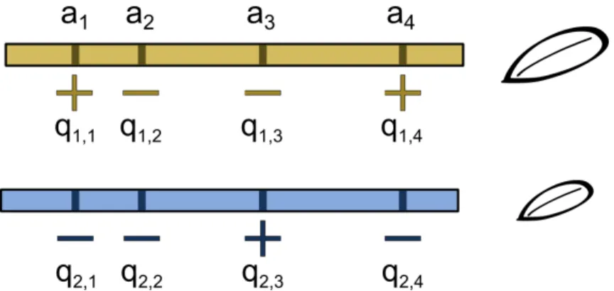
Figure 3.1: QTL data available from QTL experiments. From a QTL experiment one obtains the following data necessary for the selection test: the additive effect al that is fixed for locus l in all linesi= 1, . . . , n and the stateqi,l which can take the values ±1 and which can be different for each line (assuming that there are only two possible states). The trait value is the sum of contributions from all loci, see eq. (3.1).
Furthermore, I assume a linear Malthusian fitness (log-fitness) landscape F({ql}) =sT({ql}) =
L
X
l=1
salql, (3.2)
with the selection coefficient s. That is, if the trait is under selection (with selection strength s), the fitness increases linearly with the trait value. Fitness is the measure for the reproductive success of an individual and in population genetics fitness can be related to the probability of the establishment of an allele. Under the assumption of a linear fitness landscape, the effect of the state of a locus on both trait and fitness is independent of the states of other loci. This assumption will be examined and relaxed in section 3.6. The model contains no environmental component (quantitative traits often behave differently across different environments such as e.g. varying temperatures;
such effects are not considered here) and (for a diploid population) no dominance (a dominant allele masks the effect of a recessive allele).
I use established results from population genetics theory to derive the probability of observing the possible states q=±at a given locus. In population genetics the time evolution of a population of effective population sizeN is considered under the influence of selection, described by the fitness F, stochastic fluctuations of the reproductive process (genetic drift) and mutations (with a mutation rate µ) (L¨assig 2007). While mutations introduce new alleles into a population, selection and genetic drift finally lead to their fixation. In the case of low mutation rates (also called weak-mutation regime, which is the relevant regime for eukaryotes and most prokaryotes (Stewart and Plotkin 2013)) the time until a new mutation arises is much longer than the time needed for the fixation of a new allele. Thus, the population is monomorphic (i.e. has the same alleles in all individuals) most of the time. The other case, where several mutations segregate in one population and compete against each other is called clonal interference (Gerrish and Lenski 1998). In summary, mutations introduce new alleles at a certain rate and these mutations are either fixed in the population with a certain probability or lost.
Kimura (Kimura 1962) derived the rate of fixation of a new mutation in the weak- mutation regime. This can be done by solving the Fokker-Planck equation (2.2) in the stationary case, when ∂P(x, t)/∂t = 0. This yields the probability of fixation of a new mutation with fitness advantage ∆F as 1−exp(−2∆F)
1−exp(−2N∆F). Multiplying this fixation probability with the probability of creating an individual with this mutation in the population, which is µN, yields the substitution rate
uq→−q =µN 1−exp(−2∆F)
1−exp(−2N∆F), (3.3)
which depends on the fitness difference ∆F between the two possible states q and −q, the mutation rate µ, and the effective population size N. When considering multiple
loci, these loci do not segregate independently, but they are linked by the genetic sequence they share (called genetic linkage). There are two possible mechanisms that can break this linkage: recombination and a low mutation rate. Recombination events lead to a mixing of the genomes of different individuals. If a recombination event happens between two loci, one locus is inherited from one individual while the second locus is inherited from the other individual, which allows the loci to mix between different genomes. A low mutation rate leads to a monomorphic population where the mutations at different loci fix one by one and do not interfere. Thus, assuming the weak-mutation regime is sufficient to guarantee an independent segregation of the loci.
At low mutation rates, most loci are monomorphic at a given point in time, but may differ between lines (due to mutations that fix in a given population before the next mutation occurs). The state statistics P(q) of a locus describes the probability that this locus in a given line is in state q. In the limit of long evolutionary times between lines, this statistics no longer changes with time, so the probability P(q) is stationary (equilibrium). Under neutral evolution the genetic sequence constituting the locus is allowed to evolve freely and the equilibrium probability P(q) depends only on the number of sequence variants ωq of the locus corresponding to stateq. One obtains
P(q|Ω) = ωq ω++ω−
= exp(Ωq)
exp(Ω) + exp(−Ω), (3.4)
where I have introduced the multiplicity factor Ω = (1/2) log(ω+/ω−) of a locus which allows to capture the imbalance between + and − state in a single parameter. Loci with a high multiplicity factor have more sequence variants for the + state and thus a higher probability to be in that state. In the example with the transcription factor binding site, the number of sequences with a functioning binding site ω+ is much lower than the number of sequences without such a site ω−, leading to P(q = +1) 1 in the absence of selection (see also Figure 3.2). The multiplicity factor of a locus quantifies the asymmetry between the + and − state in the absence of selection, and correspondingly the relative number of mutations at a locus increasing or decreasing the trait.
Under selection, however, the fitness differences between the states can also create an additional bias towards one of the states. From eq. (3.3) one obtains that the ratio between the transition ratesu+→−/u−→+simplifies toµ+→−/µ−→+exp(2N∆F)∝ exp(2N∆F) forN∆F 1∆F (strong selection) and the probability to be in state q is proportional to exp(2N F) (Iwasa 1988; Berg et al. 2004; Sella and Hirsh 2005;
L¨assig 2007). The bias in mutation rates between states is exactly captured by the multiplicity factor Ω. Thus the probability of states for one locus becomes
P(q|N s,Ω, a) = exp(2N saq+ Ωq)
exp(2N sa+ Ω) + exp(−2N sa−Ω), (3.5)
Figure 3.2: Multiplicity factor of a QTL.A QTL is typically governed by a longer genetic sequence (e.g. a transcription factor binding site) and many sequence variants contribute to the two effective states q = ±. The number of sequence variants contributing to the + and −state, ω+ and ω−, can be very asymmetrically distributed. For example the + state can correspond to a functional transcription factor binding site (top) , while the − state corresponds to a non-functional binding site (bottom). Since the number of sequence variants which correspond to a non-functional binding site is much larger, there is an asymmetry between the number of sequence variants corresponding to the two states, ω− ω+. This asymmetry is contained in the multiplicity factor Ω = (1/2) log(ω+/ω−).
where I used the linear fitness function from eq. (3.2). I define a selection coefficient σ = N sa for each locus proportional to the additive effect a, which is the relevant quantity determining the strength of the selection. Since the effective population size N is usually unknown andN ands always appear together, only their product will be estimated later.
If there are n lines, each line i= 1. . . n can be in a different state q at that locus.
Thus, one locus consists of the set of states (q1, q2. . . , qn). Assuming the lines evolve independently of each other, the joint probability distribution in the limit of long evolutionary time factorizes over lines, so the state statistics for a given locus is
Pundiv(q1, . . . , qn|N s1, . . . , N sn,Ω, a) = 1
ZePni=1(2N sia+Ω)qi, (3.6) where Z = P
q1,...,qn=±1ePni=1(2N sia+Ω)qi. Here, each line can be under a different se- lection pressure si but the multiplicity factor is fixed, which reflects the same genetic basis of that locus in all lines.
Here, one needs to consider one subtlety arising from QTL analysis based on crosses between individuals from different lines: In the crosses only the effects of loci differing in their state q in at least two lines can be determined. A locus that has the same allele in all lines will also have that allele in all crosses between the lines, rendering its trait contribution invisible. This means that, independent of the number of lines, there are always two state configurations q1 =q2 =. . .=qn=±1 that cannot be observed.
From eq. (3.6) the result for the diverged loci directly follows as P(q1, . . . , qn|N s1, . . . , N sn,Ω, a) = 1
Z0ePni=1(2N sia+Ω)qi, (3.7) where I allow only diverged configurations (q1, . . . , qn) and the normalization constant has changed to Z0 = P0
q1,...,qn=±1ePni=1(2N sia+Ω)qi where the sum P0
excludes the two unobserved configurations q1 =q2 =. . .=qn =±1.
Under the linear fitness model (3.2), states at different loci are statistically inde- pendent, so the state statistics for several loci is the product of (3.7) over loci
P({qi,l}|{N si},{Ωl},{al}) =
Ldiv
Y
l=1
P(q1,l, . . . , qn,l|N s1, . . . , N sn,Ωl, al), (3.8) where the number of loci with different states in at least two lines is denoted by Ldiv. With this state statistics I can assign a probability to each of the possible configura- tions {qi,l} given the selection strength of the lines and the multiplicity factors of the loci.