Essays on Monetary Policy and Financial Regulation

Regulation

Inauguraldissertation zur

Erlangung des Doktorgrades der

Wirtschafts- und Sozialwissenschaftlichen Fakultät der

Universität zu Köln

2020

vorgelegt von

Christian Loenser, M.Sc. Wirtschaftsmathematik

aus

Castrop-Rauxel

Korreferent: Univ.-Prof. Michael Krause, Ph.D.

Tag der Promotion: 17.09.2020

The work on this dissertation during the last years was a very enriching and joyful experience. I would like to thank many people, who helped me during this time.

First of all, I would like to thank my supervisors Andreas Schabert and Michael Krause for their support and advice. Especially, I would like to express my deepest thanks and appreciation to Andreas Schabert for his excellent assistance and guidance during my doctoral studies. Working with him in our two joint research projects, that enter this thesis in Chapter 2 and 4, not only improved my understanding of economics but also my skills in scientific research. Furthermore, he intensified my interest in monetary economics already in my undergraduate studies and thereby played an important role for my decision to begin with doctoral studies in economics. By the way, while he influenced my economic thinking, his expertise regarding soccer (especially regarding Borussia Dortmund) is less appealing to me.

Furthermore, I want to thank Joost Röttger, who is my co-author in a joint research project with Andreas Schabert that enters this thesis in Chapter 4. The time we spent on our joint project was very interesting and instructive and his advice for my other projects was extremely helpful.

I would like to give thanks to the whole team of the Cologne Graduate School of Economics and the Center for Macroeconomic Research for the very nice years at the university of Cologne. Especially, I am very grateful to Erika Berthold, Ina Dinstühler, Diana Frangenberg, Sylvia Hoffmeyer and Dorothea Pakebusch for their assistance and patience with me in all administrative matters.

Lastly, I want to thank my family for their caring support. Mostly, I am deeply grateful to my wife for her loving assistance during all these years and to my newborn son who has sweetened the last days of my doctoral studies.

Castrop-Rauxel 16th February 2020

Christian Loenser

1 Introduction 1

2 Monetary Policy, Financial Constraints, and Redistribution 9

2.1 Introduction . . . . 9

2.2 A model with patient and impatient agents . . . . 13

2.2.1 The set-up . . . . 13

2.2.2 Results . . . . 15

2.3 A model with idiosyncratic risk . . . . 17

2.3.1 The set-up . . . . 18

2.3.2 A version with two representative agents . . . . 19

2.3.3 A calibrated version . . . . 22

2.4 Conclusion . . . . 33

A.2 Proof of Proposition 2 . . . . 34

B.2 Appendix to the calibrated model . . . . 35

B.2.1 Data on household debt . . . . 35

B.2.2 Transition matrix . . . . 35

B.2.3 Calculation of the stationary equilibrium under a given inflation rate . . . . 36

B.2.4 Calculation of the transition path to the new stationary equilibrium . . . . 39

C.2 Additional figures . . . . 41

3 A quantitative analysis of general equilibrium effects in a heterogeneous household economy 45 3.1 Introduction . . . . 45

3.2 The model economy . . . . 50

3.3 Quantitative analysis . . . . 54

3.3.1 Functional forms and parameters . . . . 54

VII

3.3.2 The relative magnitude of direct and indirect effects . . . . 56

3.3.3 Decomposition of indirect effects . . . . 63

3.3.4 The importance of the supply elasticity . . . . 70

3.4 Conclusion . . . . 78

A.3 Definition of equilibrium . . . . 79

A.3.1 Equilibrium under a fixed supply of durables . . . . 79

A.3.2 Equilibrium under an elastic supply of durables . . . . 79

B.3 Computational algorithm . . . . 80

B.3.1 Transition probabilities and income values . . . . 81

B.3.2 Calculation of the total effects under fixed supply . . . . 81

B.3.3 Calculation of the direct effects . . . . 85

B.3.4 Calculation of the indirect effects . . . . 85

B.3.5 Calculation of the total effects under a higher supply elasticity . . . . 86

4 Financial Regulation, Interest Rate Responses, and Distributive Effects 87 4.1 Introduction . . . . 87

4.2 A model with limited commitment and incomplete markets . . . . 92

4.2.1 A finite-horizon model with two types of agents . . . . 93

4.2.2 Pecuniary externalities and corrective policies . . . . 94

4.3 Quantitative analysis . . . 101

4.3.1 An infinite-horizon model with an endogenous wealth distribution . . . 101

4.3.2 Loan-to-value ratio . . . 104

4.3.3 Corrective taxes . . . 109

4.4 Conclusion . . . 116

A.4 Competitive equilibrium of the three-period model . . . 118

B.4 Social planner problem in the three-period model . . . 119

C.4 Definition of equilibrium for infinite-horizon model . . . 123

D.4 Computational algorithm . . . 123

D.4.1 Transition probabilities and income values . . . 124

D.4.2 Calculation of the stationary equilibrium . . . 124

D.4.3 Calculation of the transition path to the new stationary equilibrium . . . 127

E.4 Additional figures . . . 129

5 Bibliography and list of applied software 131

2.1 Consumption and welfare (in consumption units) of relatively impatient borrowers . . . . 17

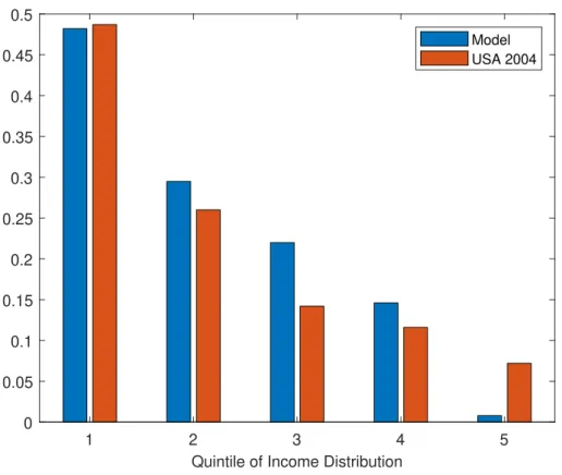
2.2 Ratios of debt to income for US income quintiles . . . . 24

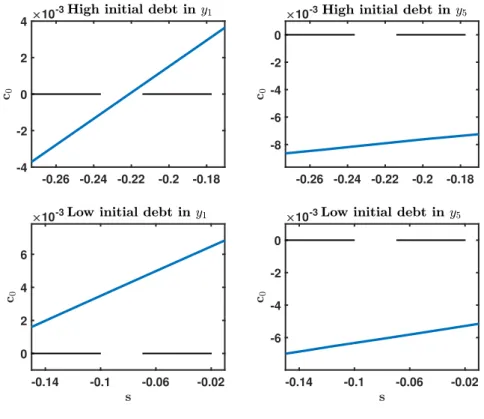
2.3 Change in the policy functions for consumption c in period 0 for an inflation reduction from 2% to -2% . . . . 25

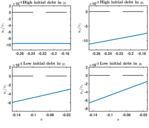
2.4 Change in the policy functions for beginning-of-period wealth s

/π in period 0 for an inflation reduction from 2% to -2% . . . . 26

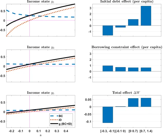
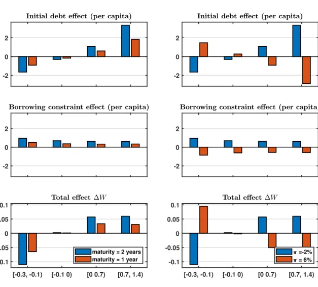
2.5 Individual welfare effects for three income states and welfare aggregated for four wealth sets 28 2.6 Welfare aggregated for four wealth sets with different maturities (left column) and different inflation rates (right column) . . . . 30

2.7 Individual welfare effects for three income states and welfare aggregated for four wealth sets under a calibration with lower autocorrelation of income . . . . 32

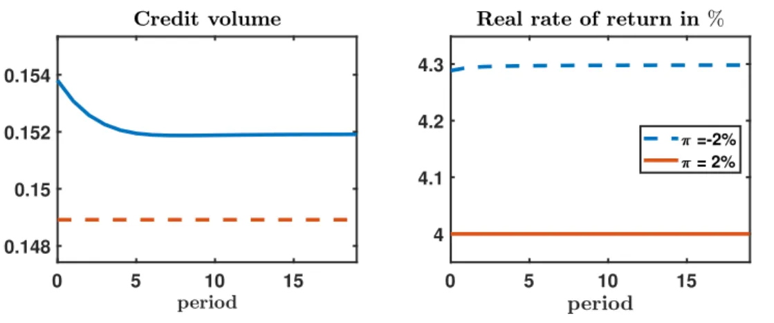
2.8 Paths of aggregate debt −s/π, and the real rate of return r

. . . . 33

2.9 Consumption and welfare (in consumption units) of relatively patient lenders . . . . 41

2.10 Policy functions for consumption and savings in period 0 . . . . 42

2.11 Policy functions for consumption and savings for stationary wealth distributions . . . . . 43

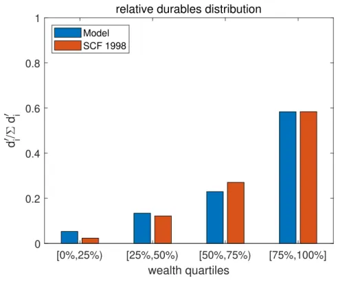
3.1 Relative durable holdings for different wealth quartiles (data vs model) . . . . 56

3.2 Relative net-wealth for different wealth quartiles (data vs model) . . . . 57

3.3 Transition path for the durables price after a positive shock on preferences for durables . 58 3.4 Percentage changes in individual decisions under a positive durables preference shock . . . 61

3.5 Percentage changes in individual decisions under an increase in the current price of durables 65 3.6 Percentage changes in individual decisions under an increase in the future price path of durables . . . . 67

IX

3.7 Percentage changes in individual decisions under an increase only in the current price of durables (dotted lines) and under an increase in both current and future prices of durables

(dashed-dotted lines) . . . . 69

3.8 Transition paths for durables price and for aggregate supply of durables after a positive durables preference shock under different supply elasticities - first part of the analysis . . 72

3.9 Percentage changes in individual decisions after a positive durables preference shock under different supply elasticities - first part of the analysis . . . . 73

3.10 Transition paths for durables price and for aggregate supply of durables after a positive durables preference shock under different supply elasticities - second part of the analysis . 75 3.11 Percentage changes in individual decisions after a positive durables preference shock under different supply elasticities - second part of the analysis . . . . 76

4.1 Relative durable holdings for different wealth quartiles (data vs model) . . . 103

4.2 Relative net-wealth for different wealth quartiles (data vs model) . . . 104

4.3 Transition paths for prices and credit after an unexpected change of loan-to-value ratio γ 105 4.4 Welfare effects conditional on income and wealth type (change in LTV) . . . 107

4.5 Transition paths for prices and credit after an unexpected change of loan-to-value ratio γ 108 4.6 Price transition paths after an unexpected tax change . . . 109

4.7 Transition path for price ratio and credit volume after an unexpected tax change . . . 110

4.8 Welfare effects conditional on income and wealth type of tax/subsidy on borrowing . . . . 111

4.9 Welfare effects of a tax/subsidy on borrowing . . . 112

4.10 Welfare effects of a Pigouvian-type tax with and without price-inelastic borrowing constraint113 4.11 Welfare effects conditional on income and wealth type of tax/subsidy on durables . . . 114

4.12 Welfare effects of a tax/subsidy on durables conditional on income state . . . 115

4.13 Aggregate welfare effects of a tax/subsidy on durables . . . 116

4.14 Bond holdings and welfare for y

(change in loan-to-value ratio γ) . . . 129

4.15 Durable holdings and welfare for y

(tax on durables)) . . . 129

2.1 Average after tax income, average value of these debt holdings, and debt-to-income for income quintiles in 2004 (in 2004 dollars) . . . . 35 3.1 Model parameters in chapter 3 . . . . 54 3.2 Summary of the qualitative impact of different indirect effects on households’ current

decisions . . . . 66 4.1 Model parameters in chapter 4 . . . 102

XI

Introduction

How do monetary policy and financial regulation affect economies populated by heterogeneous households under financial frictions? The existing theoretical literature that analyzes the impact of these policy inter- ventions on household saving and consumption typically applies relatively stylized frameworks concerning the role of household heterogeneity and financial frictions. While there is a growing branch of the lit- erature examining monetary policy effects in heterogeneous agent economies under incomplete markets, these studies are typically silent on the role of financial frictions for the monetary transmission (e.g.

Debortoli and Gali (2018), Kaplan et al. (2018) or Auclert (2019)). In contrast, studies on the effects of financial regulation on household behavior emphasize the importance of these frictions while the focus is typically on relatively stylized specifications of household heterogeneity (e.g. Bianchi (2011), Bianchi and Mendoza (2018) or Jeanne and Korinek (2019)).

As an important contribution to this literature, my doctoral thesis consists of three self-contained chapters that examine how heterogeneous households interact in quantitative models of household saving and consumption under financial frictions and how monetary policy and financial regulation affect these economies. This thesis finds that heterogeneous household economies with financial frictions give rise to a novel monetary transmission channel as well as to important ways financial interventions affect these economies that are neglected in the existing literature.

Chapter 2 addresses the effects of monetary policy in this type of framework. The research in this chapter is joint work with Andreas Schabert and provides a novel mechanism of monetary policy non- neutrality. The monetary transmission to the real economy is one of the most discussed research areas in economics.

In monetary policy analyses, the commonly used benchmark models typically disregard the role of household heterogeneity (see e.g. Woodford (2003)). Empirical studies, however, show that the

1See for example Woodford (2003).

1

sensitivity of consumption to interest rate changes in these types of models is typically too small to be reconciled with empirical evidence (e.g. Campbell and Mankiw (1989), Yogo (2004) or Canzoneri et al.

(2007)). In recent years, therefore, a growing literature has started to re-analyze the effects of monetary policy in models with heterogeneous agents under incomplete markets (e.g. Debortoli and Gali (2018), Kaplan et al. (2018) or Auclert (2019)). These studies show that the transmission of monetary policy to the real economy depends to relatively large extent on the way agents’ heterogeneity is modelled.

This heterogeneity, for example, affects the monetary transmission by changing the relative magnitude of direct and indirect (general equilibrium) effects of monetary policy (e.g. Kaplan et al. (2018)) or by generating important redistributive effects across different income groups (e.g. Auclert (2019)).

Based on broad empirical evidence, the vast majority of studies on monetary policy effects on house- hold saving and consumption considers nominal rigidities in goods and labor markets as the main sources of monetary non-neutrality.

In contrast, the role of financial frictions in this regard has received much less attention in the literature, even though their existence is undisputed.

Financial frictions, for example, can rationalize the existence of borrowing constraints whose role for household decisions is emphasized by numerous empirical and theoretical studies.

While these financial constraints in models with incomplete markets are crucial drivers of household behavior as well as important sources of inefficiencies, the litera- ture typically disregards the interaction of these constraints with monetary policy.

However, if monetary policy is able to influence borrowing constraints, it might exert important redistributive effects that would complement the above mentioned studies on monetary policy in economies with heterogeneous agents.

Therefore, chapter 2 addresses this interaction of monetary policy and borrowing constraints in a het- erogeneous household economy calibrated to match distributional targets based on US data and thereby works out a novel mechanism of monetary non-neutrality which is based on borrowing constraints related to current income. This type of financial constraint induces redistributive effects of monetary policy among heterogeneous households that exist even under flexible goods prices.

The central elements of this analysis are that only nominal debt is available and that outstanding debt is limited by current income. In principal, this type of constraint can be rationalized by the inability of borrowers to commit to repayment. Under a repudiation-proof debt contract, outstanding debt is then restricted by current income. Such limits for unsecured debt, for which broad empirical evidence exists (see e.g. Jappelli (1990) or Lian and Ma (2019)), do not account for expected price changes until maturity, implying that monetary policy can alter the real terms of borrowing. In our analysis, we introduce this

2This is true for monetary policy analyses that neglect the role of household heterogeneity as Woodford (2003) or Christiano et al. (2005) as well as for studies that acknowledge this heterogeneity as Kaplan et al. (2018).

3See for example the extensive survey of the role of financial frictions in macroeconomics in Brunnermeier et al. (2013).

4See e.g. Diaz and Luengo-Prado (2010), Saiz (2010), Mian and Suffi (2011) or Guerrieri and Iacoviello (2017)).

5Note that there does exist a borrowing constraint in Kaplan et al. (2018). This non-microfounded constraint, however, induces no additional monetary transmission channels in their study.

type of borrowing constraint into a Huggett (1993)-type heterogeneous agent economy with idiosyncratic endowment and non-state contingent bonds, calibrate this model to US data and examine the effects of an exogenously given change in the inflation rate on saving and consumption of heterogeneous households.

Given this borrowing constraint, a reduction in inflation tends to increase the maximum amount of debt that can be issued, while it also raises the beginning-of-period stock of debt to be repaid. The impact of inflation depends on the probability of borrowers to be unconstrained at maturity which especially depends on the persistence of the endowment process. The lower this probability is, the smaller is the beneficial effect of lower inflation for borrowers. The effect of monetary policy on the debt limit is opposed to the classic debt deflation effect when borrowers are initially indebted. While a reduction in the inflation rate increases the debt limit, the real value of initial debt obligations rises, too. The overall effect is therefore ex-ante ambiguous and depends on the initial debt/wealth position as well as the willingness to borrow. The study shows that lower inflation particularly benefits agents with low initial debt by relaxing effective borrowing constraints, whereas highly indebted borrowers suffer from the dominant debt deflation effect. For our benchmark calibration, we find that aggregate welfare losses due to the inflation reduction via the (conventional) effects of initial debt deflation are reduced by 83%

via the effects induced by the borrowing constraint. If the persistence of the endowment process is low enough, a reduction of the inflation rate can even enhance aggregate welfare.

Chapter 3 and 4 shift the focus towards the analysis of financial regulation in an economy with

an empirically relevant specification of borrowing constraints and household heterogeneity. Research

on financial regulation in macroeconomic frameworks intensified in the aftermath of the last financial

crisis. The severe consequences of the disruptions in financial markets convinced most economists to

complement the microprudential approach to financial regulation by a macroprudential one that focusses

on the financial system as a whole (see e.g. Hanson et al. (2011)). The literature on macroprudential

financial regulation especially addresses the interaction between de-leveraging and asset prices induced

by price-dependent collateral constraints. Given that the scope to borrow against collateral crucially

depends on the price of (pledgeable) assets, borrowers tend to de-leverage in states where asset prices

fall, giving rise to a financial amplification mechanism (see e.g. Kiyotaki and Moore (1997)). Given

that (borrowing) agents do not internalize the impact of their behavior on prices, they might tend to

overborrow. This pecuniary externality with regard to the collateral price provides a straightforward

rationale for a macroprudential approach to financial regulation as for example shown by Lorenzoni

(2008), Bianchi (2011), Bianchi and Mendoza (2018) or Jeanne and Korinek (2019). These studies then

typically find that the pecuniary externality regarding the collateral price can be corrected by an ex-ante

policy that constrains or dis-incentivizes borrowing, such as a reduction in the loan-to-value ratio or a

Pigouvian tax on borrowing.

While these studies focus on the role of financial frictions - especially of price-dependent borrow- ing constraints - the analyzed frameworks abstain from empirically relevant specifications of household heterogeneity. They usually employ infinite-horizon small open economy models (based on Mendoza (2010)), where a representative domestic agent borrows from abroad, or three-period closed economy models with distinct types of agents, who either borrow or lend (e.g. Lorenzoni (2008) or Jeanne and Korinek (2019)). The focus of these analyses is on the effects of collateral externalities that result from endogenous collateral prices in borrowing limits. Distributive externalities, however, which are a second type of pecuniary externalities that generally matters for (in-)efficiency in economies under financial fric- tions (see e.g. Davila and Korinek (2018)), are irrelevant in these studies. Distributive effects arise when the relative price at which agents trade goods or assets changes. This price adjustment then redistributes funds among buyers and sellers and thereby influences relative demand. The studies on financial regu- lation mentioned above, however, focus on models in which only a representative (domestic) borrower is able to hold the collateral asset. In these frameworks, therefore, changes in collateral prices do not induce distributive effects across lenders and borrowers. Furthermore, given that the real interest rate on bonds is fixed in these studies, distributive effects via changes in the real rate also do not exist.

While these studies analyze policy interventions in relatively stylized frameworks, my thesis examines financial regulation in an economy with both - an empirically relevant specification of borrowing con- straints as well as of household heterogeneity.

The framework is a Huggett (1993)-type heterogeneous agent economy extended by an occasionally binding collateral constraint and by a durable good, that has a dual role as a non-financial (collateral) asset and as a utility providing consumption good.

The model is calibrated to match several aggregate and distributional targets based on US data following Diaz and Luengo-Prado (2010). In this framework, changes in market prices induce not only collateral effects but also distributive effects via adjustments in collateral prices and the real interest rate.

The magnitude of pecuniary externalities and - as a consequence - the role of policy interventions in this type of model especially depend on the following two aspects. Firstly, it depends on the sensitivity of market prices. The higher the price sensitivity is, the more important are pecuniary externalities. A key driver of the sensitivity of the collateral price is the elasticity of aggregate supply of the collateral asset with respect to collateral price changes. The lower this elasticity of supply is, the larger is the price sensitivity. In the model applied to analyze financial interventions in this thesis - as in the studies

6Note that the empirical literature shows the existence of a pronounced observed and unobserved heterogeneity among households (e.g. Krueger et al. (2016a) or Hai and Heckman (2017)) and that theoretical studies find that this heterogeneity is important for the evolution of aggregate quantities and prices (e.g. Krusell and Smith (1998)) as well as for normative questions (e.g. Kaplan and Violante (2014)).

7Since the 1980s, household debt secured by durable consumption goods (like vehicles or especially residential real estate) has accounted for more than90%of US household debt in the United States (see Hintermaier and Koeniger (2016)).

mentioned above - the supply of the collateral asset is fixed such that the price sensitivity is relatively strong. Secondly, the impact of financial regulation depends on the relative magnitude of collateral and distributive effects of price changes which can have opposing effects that are not equally distributed among households. In the model in this thesis - in contrast to the studies mentioned above - the role of both types of price effects for policy interventions is examined.

Before chapter 4 analyzes the effect of financial regulation on household saving and consumption, chapter 3 at first examines the role of the price sensitivity of the collateral asset and the relative magnitude of collateral and distributive effects on household decisions in this type of framework absent any policy interventions. To do so, this study examines the relative magnitude of direct effects and indirect ones arising from changes in the collateral price on household saving and consumption induced by a shock on household preferences for the durable good. The direct effects of the shock are those that operate in the absence of any changes in market prices. In general equilibrium, additional indirect effects on households’

behaviour arise from changes in market prices that emanates from the direct effects.

The magnitude of the shock is set to induce an increase in the price of durables in the impact period which is close to the impulse response of the housing price under a shock on housing preferences in the estimated model in Guerrieri and Iacoviello (2017). The motivation to analyze shocks on preferences for the durable consumption good is based on quantitative studies which find that house price movements can be explained to a large extent by housing preference shocks (see e.g. Liu et al. (2013), Berger et al.

(2017) or Guerrieri and Iacoviello (2017)). The focus of this study is on the fluctuations of the collateral price - as in the studies mentioned above - while the real interest rate is time-invariant.

At first, the relative magnitude of direct and indirect effects is analyzed in a model version with a fixed aggregate supply of collateral. Empirical studies, however, find that growth rates in prices of housing, which is typically the dominant component of household wealth in the US (see e.g. Li and Yao (2007)), are not homogeneous across areas in the US in the 1980s and from 2002 to 2006 and that this heterogeneity is driven to a relatively large extent by heterogeneous supply elasticities of housing (see e.g.

Glaeser et al. (2008), Mian and Sufi (2009), Saiz (2010) or Mian et al. (2013)). Areas with a relatively inelastic housing supply, due to e.g. geographical limitations, experienced relatively high growth rates in house prices in the 1980s and from 2002 to 2006 whereas areas with a relatively elastic supply had lower growth rates.

Given the high share of housing in wealth of the household sector, household borrowing and consumption depends to a relatively large degree on the sensitivity of housing prices and therefore on the elasticity of housing supply (see e.g. Mian and Sufi (2011, 2013)). For example, those areas

8Saiz (2010) constructs an objective index measuring the possibility to expand new housing in metro areas. If land- topology in a metro area is such that expansion from the center is restricted - for example by hills, oceans or lakes - this area gets a low housing supply elasticity score.

that experienced relatively high growth rates in house prices due to a relatively inelastic housing supply typically also experienced larger increases in home-equity borrowing and thereby also in consumption.

These results imply that the model version with a fixed supply of durables generates an upper bound for the importance of indirect price effects. Therefore, the relative magnitude is re-analyzed in a model version with a more elastic supply in which the importance of price effects is reduced.

The analysis finds that in the considered type of model changes in the price of the collateral asset are not only a key driver of household behavior under a fixed aggregate supply of collateral but also when the price sensitivity is relatively strongly reduced by increasing the elasticity of aggregate collateral supply.

This result suggests that the large scope for financial regulation under fixed collateral supply - derived in chapter 4 as well as in the studies above - should also exist under less extreme assumptions concerning the supply elasticity. Furthermore, the study finds that households’ saving and consumption behavior are especially driven by distributive effects and only to lower extent by collateral ones. This result is in contrast to the importance of collateral effects in the studies on financial regulation with relatively stylized specifications of household heterogeneity. While these studies focus on the collateral price effect, the results from chapter 3 suggest that policy interventions, that address pecuniary externalities, should also take into account distributive effects of price changes. This finding i.a. motivates the analysis of financial regulation in a heterogeneous household economy in chapter 4 where - in contrast to the existing studies o financial regulation - both price effects - collateral and distributive effects - emerge.

Chapter 4 is joint work with Joost Röttger and Andreas Schabert and examines financial regulation and corrective policies in a heterogeneous agent economy similar to one analyzed in chapter 3. In contrast to chapter 3 and also in contrast to the literature on financial regulation mentioned above, the real interest rate in this framework is time-variant such that changes in two market prices - the price of durables and the real interest rate - are important for household saving and consumption. As a novel contribution, we analyze the impact of financial regulation in a framework in which household decisions are not only affected by collateral effects but also by distributive effects via changes in the collateral price and in the real interest rate.

In the first part of chapter 4, we solve for Pigouvian-type taxes/subsidies in debt and asset markets that

can correct the different pecuniary externalities and thereby implement a constrained efficient allocation

in a simplified three-period model. The framework analyzed in our study is an extension of the model in

Davila and Korinek (2018) by adding a price dependent borrowing constraint in the initial period. The

analysis then shows that without further information on preferences and the distributions of bonds and

durables it is in general unclear whether the implementation of a constrained efficient allocation requires

taxes or subsidies on debt and durables.

In the second part of chapter 4, we therefore analyze the effects of given policy interventions in a quantitative model calibrated to US data. While existing studies, as explained above, focus on collateral effects, this analysis reveals that the welfare consequences of policy interventions in credit and asset markets mainly depend on distributive effects of price changes, i.e. distributive effects of collateral price changes and of changes in the real interest rate.

The analysis finds that a loan-to-value reduction - an instrument typically suggested in the litera-

ture on financial regulation - benefits only few unconstrained borrowers and reduces social welfare. A

Pigouvian-type debt-tax/savings-subsidy, however, raises collateral prices and lowers interest rates, which

stimulates borrowing and generates welfare gains for almost all income groups. The analysis suggests that

in heterogeneous agent economies especially interventions in savers’ decisions are beneficial while these

instruments are typically ineffective in the macroprudential studies mentioned above. Overall, collateral

effects are of minor importance in this framework and interest rates rather than asset price responses are

decisive for welfare effects of corrective policies.

Monetary Policy, Financial Constraints, and Redistribution

This chapter is based on Loenser and Schabert (2019).

2.1 Introduction

Based on broad empirical evidence, the vast majority of studies on monetary policy effects considers nominal rigidities in goods and labor markets as the main sources of monetary non-neutrality. In contrast, the role of financial frictions in this regard has received much less attention in the literature, even though their existence is undisputed. Debt is typically issued in nominal terms and in a non state- contingent way, such that changes in the price level can alter real payoffs. This transmission channel of unexpected monetary policy (the so-called Fisher debt deflation channel) is well-established and has been examined in several studies.

In this paper, we examine a novel channel of monetary transmission via financial constraints expressed in nominal terms.

Thereby, monetary policy exerts redistributive effects, which complements other recently-studied general equilibrium effects of monetary policy on heterogeneous agents (see Kaplan et al. (2018) or Auclert (2019)).

The central elements of our analysis are that only nominal debt is available and that outstanding debt is limited by current income. The latter assumption is motivated by empirical evidence provided by numerous studies that current income or earnings serve as a relevant limit for unsecured debt (see e.g.

1For example, Doepke et al. (2015) or Auclert (2019) are recent contributions to this literature. They further provide comprehensive overviews over studies on distributional effects of monetary policy.

2Gariga et al. (2017) examine the transmission of monetary policy via nominal rigidities induced by fixed-rate and adjustable-rate mortgage contracts.

3Kaplan et al. (2018) show that indirect (general equilibrium) effects via labor income of heterogeneous households can outweight direct effects of monetary policy, in particular, via intertemporal substitution.

9

Japelli and Pagano (1989), Jappelli (1990), Duca and Rosenthal (1993), Del Río and Young (2006), Choi et al. (2018), Dettling and Hsu (2018), Drechsel (2019) or Lian and Ma (2019)) and by various theoretical studies that focus on current – rather than on future – factors that limit debt. In particular, studies on fire sales consider the impact of asset sales on their current period value (see e.g. Stein (2012), Woodford (2016), Davila and Korinek (2018)), inducing debt deleveraging by tightening the limit for end-of-period debt within the same period. Moreover, studies that rationalize macroprudential regulation by pecuniary externalities consider borrowing limits that restrict end-of-period debt by current period income valued at current relative prices (see e.g. Bianchi (2011), Benigno et al. (2016), Korinek (2018) or Schmitt-Grohe and Uribe (2019)).

This type of constraints can principally be rationalized by the inability of borrowers to commit to repayment. If debt can be renegotiated after issuance, borrowers – who cannot commit – might make a take-it-of-leave-it offer to reduce the value of debt. Suppose that lenders who reject this offer, can seize borrowers’ wealth. When assets are not available, as considered in this paper, an offer will thus be accepted when the repayment value of debt does not exceed borrowers’ available income. Under a repudiation-proof debt contract, outstanding debt is then restricted by current income.

We explore implications for monetary policy and its redistributive effects under fully flexible goods prices when repayment of unsecured debt is constrained by current income. Apparently, the debt limit in terms of commodities at maturity can then be affected by price level changes and thereby by monetary policy. To make this argument more transparent, consider a nominal repayment S

that is contracted in t at the period t price Q

and due in t + 1. Suppose that it is limited at issuance by current income, S

≤ P

y

, where y

denotes an exogenous real income and P

the price level in period t. Then, real debt repayment in terms of commodities in period t + 1, x

= S

/P

, has to satisfy x

≤ y

/π

, where π

denotes the inflation rate π

= P

/P

. Thus, a change in the inflation rate alters the effective debt limit, i.e. the maximum debt in terms of commodities at maturity.

To understand the macroeconomic effects of monetary policy under a debt limit based on current income, consider for example an unexpected permanent increase in the inflation rate. On the one hand, a higher inflation rate implies the debt limit to shrink in terms of commodities at maturity. Given that this reduction in the value of debt at maturity is internalized by lenders, they also demand a lower debt price Q

at issuance, which tends to reduce the maximum amount of funds that can be borrowed. On the other hand, there is a beneficial effect of the reduced debt repayment value in terms of commodities at

4Other theoretical studies, which consider current income as debt limits are, for example, Laibson et al. (2003) or Mendoza (2006).

5Note that such a constraint relates total outstanding debt to income and therefore differs from payment-to-income ratios that are relevant for mortgage (see Corbae and Quintin (2015) or Greenwald (2018)).

6If debt limits instead account for expected future price changes, debt limits would be specified in terms of commodities at maturity, implying that monetary policy does not affect the effective tightness of the borrowing constraints. Then, monetary policy matters just due to the (conventional) effects of initial debt deflation.

maturity, which is in fact identical to the conventional debt deflation effect in the initial period. Hence, the increase in inflation tends to reduce the maximum amount of debt that can be issued (debt limit effect ) as well as the stock of debt to be repaid (debt deflation effect ). The beneficial debt deflation effect is opposed to the impact on the effective debt limit. Thus, the effect of higher inflation on borrowers’

overall consumption possibilities and welfare is ex-ante ambiguous, and particularly depends on the likelihood that the borrowing constraint is binding and on the borrowers’ initial debt level. Moreover, when borrowing decreases due to a tighter effective debt limit under a higher inflation rate, the real interest rate and thus the real cost of borrowing tend to fall.

To assess the overall impact of changes in the inflation rate, we examine two distinct models. We first consider the highly stylized case of a stationary equilibrium of an economy where agents permanently differ by their degree of patience (as for example studied by Kiyotaki and Moore (1997)). Relatively impatient agents tend to frontload consumption and are willing to borrow from more patient agents up to the maximum amount. A higher inflation rate then leads to the two effects described above: Debt repayment as well as the amount of newly issued debt are reduced. In this economy, where agents never switch types (borrower/lender), the beneficial debt deflation effect dominates the debt limit effect, such that borrowers are better off with higher inflation rates. In contrast, if the borrowing limit were exogenously tightened, say, by an exogenous reduction of the fraction of seizable income, borrowers’

welfare would tend to decrease. The apparent reason is that this impulse lacks the beneficial effect from a reduction of the initial debt burden, while it reduces initial and future consumption possibilities of borrowers due to a tighter effective debt limit.

For the main part of our analysis, we focus on a second – less stylized – framework and apply an incomplete market model (see Huggett (1993)). Agents differ with regard to their random individual income, while they are equally impatient.

When an agent draws a very low realization of income, he is willing to borrow up to the debt limit. The adverse (beneficial) effect of a higher (lower) inflation rate that tends to lower (raise) the effective debt limit and, correspondingly, the maximum amount of borrowed funds at issuance might then outweigh the beneficial (adverse) debt deflation effect. This is actually the case when the probability of drawing again a low realization of individual income at maturity is small enough, such that the marginal valuation of funds at issuance is sufficiently higher than the expected marginal valuation of funds at maturity. Ex-ante, a borrower tends to prefer a lower inflation rate and

7Notably, this pecuniary externality (non-trivially) applies also for the opposite case of lower inflation, which increases the maximum debt repayment: Given that agents do not internalize how their demand for funds affects the real interest rate, a lower inflation rate can cause an increase in debt due to borrowers exploiting the higher debt limit, which tends to increase the real cost of borrowing. A related externality with regard to the real interest rate is discussed by Smith (2009).

8This set-up closely relates to Auclert’s (2019) incomplete market model, which he uses to examine redistribution of monetary policy. In contrast to our model, the borrowing constraint in his model limits issued debt rather than outstanding debt, such that the changes in inflation does not alter the effective debt limit.

thus a higher effective debt limit even with the higher debt repayment, if he has a relatively high valuation of funds when debt is issued.

We examine two versions of the incomplete market model with idiosyncratic risk. For the first version, we assume that preferences are linear-quadratic and that income shocks ensure that the borrowing con- straint always binds for borrowers, facilitating aggregation and allowing for the derivation of analytical results. Under these assumptions, the competitive equilibrium of the heterogenous agents economy can be characterized in terms of a representative borrower and a representative lender. For this economy, we show analytically that a reduction in the inflation rate can enhance welfare of the representative borrower if the autocorrelation of income shocks is sufficiently low, which tends to raise the gain from the debt limit effect relative to the debt deflation effect. The reason is that a constrained borrower is under a lower autocorrelation of individual income less likely to be constrained at maturity, such that the expected marginal utility of consumption at maturity is lower than the marginal utility of consumption at issuance. With this favorable effect for constrained agents, monetary policy can in principle enhance aggregate welfare by lowering inflation.

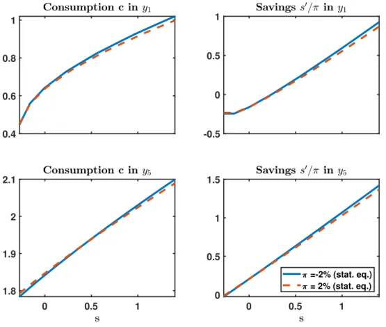
To quantitatively assess the effects of changes in the inflation rate, we apply a second version of the model, imposing less restrictive assumptions. Specifically, we consider a standard CRRA utility function, long-term debt, and a more realistic income process, such that the borrowing constraint is not permanently binding. Given that this version cannot be solved analytically, we calibrate the model to match characteristics of US postwar data and solve it numerically. The calibration is based on an inflation rate of 2%. We then assume that the central bank reduces the average inflation rate to -2%. We find that borrowers with a high initial debt position suffer most from lower inflation, given that the debt deflation effect is dominant for them. In contrast, borrowers who are initially less indebted gain from lower inflation due to a dominant debt limit effect. Apparently, a household with positive wealth benefits from both effects when the central bank reduces the inflation rate: Initial real wealth increases as well as debt limits in future periods in which they might be constrained. For our benchmark calibration, we find that aggregate welfare losses due to the inflation reduction via the (conventional) effects of initial debt deflation are reduced by 83% via the effects induced by the borrowing constraint.

To assess the sensitivity of these results, we vary the maturity of debt, examine an equally-sized increase (instead of a reduction) in inflation, and we re-calibrate the model for an alternative income process with lower autocorrelation. Firstly, a reduction of debt maturity leads to an almost proportional

9Studies on monetary policy in incomplete market economies with zero debt and fixed borrowing limits typically find effects of higher inflation rates that are beneficial for borrowers (see e.g. Akyol (2004), Algan and Ragot (2010), or Kryvtsov et al. (2011)).

10As a measure for aggregate welfare, we apply agents’ ex-ante expected lifetime utility, which relates to an utilitarian welfare measure.

reduction of the welfare effects. As described by Doepke and Schneider (2006), debt deflation effects of non-transitory inflation changes increase with the maturity of nominal debt. Likewise, fixing nominal payments for longer terms is crucial for the effects of monetary policy via nominal rigidities induced by fixed-rate mortgage contracts (see Gariga et al. (2017)). The debt limit effect is also enhanced with higher maturities, which – like a lower autocorrelation of income – increase the likelihood that borrowers are unconstrained at maturity. Secondly, we find that an increase in inflation leads to almost symmetric effects compared to an equally-sized inflation reduction. These effects are slightly less pronounced, given that the distortionary effects of the borrowing constraint are reduced under higher inflation rates. Finally, we also consider a lower autocorrelation for the income process, as suggested by Guvenen (2007) for the US and by Floden and Line (2001) for Sweden. Re-calibrating the model for Guvenen’s (2007) estimates, we find that aggregate welfare (slightly) increases for a reduction in the inflation rate, consistent with the analytical results derived for the simplified version of the model.

In Section 2, we examine the redistributive effects of monetary policy in a stylized model with two agents which are characterized by different degrees of impatience. In Section 3, we apply a model where heterogeneity of agents, instead, originates from idiosyncratic income shocks, and examine the inflation effects analytically as well as numerically. Section 4 concludes.

2.2 A model with patient and impatient agents

Before we examine financial frictions for monetary policy effects in a Huggett (1993) type model (see Section 2.3), we analyze the effects in a more stylized model. We assume that two types of agents differ with regard to their degree of patience induced by different discount factors (as in Kiyotaki and Moore (1997)). The patient agents with the higher discount factor will permanently be lenders and the impatient agents with the lower discount factor will permanently be borrowers. The persistence of agents’ types will be the main difference between this model and the model in Section 2.3, where agents might switch roles in the credit market depending on their particular income draws and their endogenous wealth positions.

2.2.1 The set-up

There is a continuum of infinitely lived agents of mass two, who have equal income from an exogenous

labor supply, consume and trade one-period nominal non-state contingent discount bonds at the issuance

price 1/R

(= Q

), paying one unit of currency in period t. For simplicity, we neglect uncertainty and

disregard holdings of fiat money, which can be interpreted as the limit case of a cashless economy, while

we assume that money only serves as a unit of account (see also Sheedy (2014) or Auclert (2019)).

Households maximize the present value of utilities P

t=0

(β

)

u(c

) where c

is consumption of agent i and i = l (i = b) is the index of lenders (borrower), who constitute half of the population. The parameter β

is the discount factor of agent i and satisfies β

< β

< 1. The utility function is identical for all agents and satisfies u

> 0 and u

< 0. Agent i’s budget constraint in nominal terms is given by

P

c

= −(S

/R

) + S

+ P

y

, (2.1)

where P

denotes the price level, S

denotes nominal debt with S

> 0 and S

< 0. The endowment y

will be identical for all agents, y

= y

. In each period, agents first trade in the asset market before they enter the goods market.

As the central element of our analysis, we consider that debt is restricted by current income, for which several studies found empirical support.

To rationalize this observation, we consider that agents cannot commit to repay debt. We assume that debt can be renegotiated after issuance. Borrowers might then make a take-it-of-leave-it offer to reduce the value of outstanding debt. Lenders who reject this offer, can take borrowers to court and can seize their available income up to a fraction γ < 1 (due to imperfections in legal enforcement). Hence, a repudiation-proof debt contract restricts debt repayment to γP

y

, leading to the following borrowing constraint

− S

≤ γP

y

. (2.2)

In real terms, i.e. in terms of period t commodities, the budget and borrowing constraints are given by c

= −s

/R

+ s

/π

+ y

and −s

≤ γy

, where π

:= P

/P

denotes the inflation rate and s

:= S

/P

the real value of wealth at the end of the period t, which is a predetermined state variable in t + 1. Accordingly, real end-of-period debt s

is constrained by a fraction of real income in period t, y

. Yet, when debt matures, prices might have changed, such that the real value s

has to be adjusted by the inflation rate to account for real debt burden in terms of commodities at maturity, i.e.

s

/π

= S

/P

. Accordingly, the borrowing constraint −S

/P

≤ γy

/π

shows that a higher inflation rate reduces the limit for debt repayment in terms of commodities at maturity t + 1.

Maximizing lifetime utility subject to the budget- and borrowing constraints, leads to the borrowers’ and lenders’ first order conditions given by

11Examples are Japelli and Pagano (1989), Jappelli (1990), Duca and Rosenthal (1993), Del Río and Young (2006), Choi et al. (2018), Dettling and Hsu (2018). Lian and Ma (2019) and Drechsel (2019) further provide evidence that firms’

borrowing is constrained by their earnings.

12Studies where borrowing is also constrained by the current value of income, are for example Laibson et al. (2003), Mendoza (2006), Bianchi (2011), Benigno et al., (2016), Korinek (2018), Schmitt-Grohe and Uribe (2019).

u

(c

)/R

= β

u

(c

)π

+ ζ

, (2.3)

u

(c

)/R

= β

u

(c

)π

, (2.4)

where ζ

denotes the multiplier on the borrowing constraint (2.2), which is irrelevant for lenders. Further, the associated complementary slackness condition, ζ

(γy

+ s

) ≥ 0, holds.

In this cashless economy, the central bank can control the nominal interest rate via a channel system.

Given that changes in the nominal interest rate will affect the (expected) inflation rate, we will assume, for convenience, that the central bank controls the inflation rate by setting the interest rate in order to meet specific inflation targets, as for example in Sheedy (2014). Given that there is no aggregate uncertainty, we will focus on constant inflation targets, π > 0 . Notably, the inflation choice might imply values for the nominal interest rate for which the zero lower bound, R

≥ 1, is binding.

The equilibrium is then a set of sequences {c

, c

, s

, s

, R

, ζ

≥ 0}

for a given constant inflation rate π > 0 and a given constant endowment y

= y > 0 satisfying (2.3) and (2.4), c

=

−(s

/R

) + (s

/π) + y, c

+ c

= 2y, −s

≤ γy, ζ

(γy

+ s

) ≥ 0, and −s

= s

, given

−s

= s

. The real interest rate satisfies (2.4) and will be strictly positive in a long-run equilibrium, i.e. it equals the inverse of the lenders’ discount factor, R/π = 1/β

> 1. Given that β

< β

, borrowers will be constrained in a long-run equilibrium, ζ

> 0 (see 2.3).

2.2.2 Results

We now examine the effects of a permanent change in the inflation rate in this simple economy. Specif- ically, we consider an unanticipated permanent inflation shock in period t = 0, where borrowers are endowed with beginning-of-period wealth s

= S

/P

. Suppose that the latter is sufficiently close to its steady state value, such that the economy will be in the steady state in period t ≥ 1. Using the steady state real interest rate, R/π = 1/β

, and that borrowers are always constrained, s

= −γy, the borrowers’ budget constraint, c

= −s

R

+ s

π

+ y, implies initial consumption and steady state consumption (in t ≥ 1) to satisfy

c

= [s

/π]

| {z }

A.)initial debt deflation effect

+ γ [y/R

(c

, c

, π)]

| {z }

B.)initial debt limit effect

+ y, (2.5)

c

= − [γy/π]

| {z }

C.)debt deflation effect

+ [γy/π]β

| {z }

D.)debt limit effect

| {z }

<0

+ y, ∀t ≥ 1, (2.6)

where the beginning of period stock of debt, s

< 0, is given. Consider an unexpected permanent increase in the inflation rate in period 0. This tends to increase borrowers’ consumption in period 0 according to the initial debt deflation effect (see A. in 2.5), which is independent of the borrowing constraint. At the same time, higher inflation tends to reduce c

due to the initial debt limit effect (see B.). Specifically, a higher inflation rate causes lenders’ to demand a higher nominal interest rate according to their credit supply schedule (2.4), such that the amount of funds raised at issuance γy/R

decreases. From t = 1 onwards, the economy is in the steady state, where the real interest satisfies R/π = 1/β

> 1. As in t = 0, the debt deflation effect (C.) tends to raise and the debt limit effect (D.) tends to reduce borrowers’ consumption under higher inflation (see 2.6). In contrast to the initial period, the latter effect is unambiguously weaker than the former, as debt is rolled over at a constant positive interest rate. Hence, borrowers’ consumption strictly increases with higher inflation for t ≥ 1.

Two aspects should be noted here.

Firstly, a higher inflation rate would have no further effect on borrowers’ consumption than the initial debt deflation effect (A.), if the borrowing limit were specified terms of commodities in period t + 1. If borrowing were instead limited by −S

≤ γP

y

⇐⇒ −s

/π

≤ γy

, borrowers’ consumption in t ≥ 1 (in which the economy is in a steady state) would be given by c

= −γy (1 − β

) + y. Monetary policy would then be neutral in the steady state, since the debt limit is not affected by price changes.

Secondly, a permanent reduction of the fraction of seizable income γ starting in period t = 0, which for example might be imposed by regulation, is actually not equivalent to an increase in the inflation, which can be seen from (2.5). The reason is that a change of γ in t = 0 cannot affect real initial wealth s

(for which γ would already have to be changed in t = −1).

For demonstrative purposes, we provide quantitative results for the effects of inflation. To abstract from transitional dynamics, we assume that borrowers are initially endowed with the steady state stock of debt, s

= −γy. Notably, the latter assumption implies that the borrower will be in a steady state in all periods t ≥ 0 with s

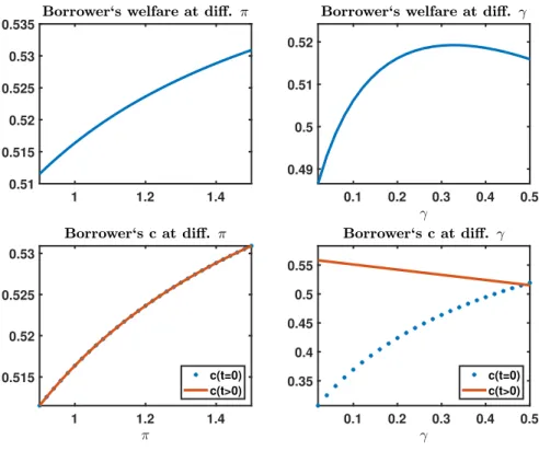
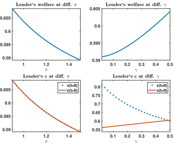
= −γy regardless of the inflation rate. Figure 2.1 shows the steady state effect of the inflation rate π and the parameter γ on borrower’s consumption and welfare for the period t = 0 and t > 0. The corresponding effects on lenders are shown in Figure 2.9 in Appendix C.2.

We compute welfare of borrowers by v

= P

t=0

β

u(c

) = u(−γ(y/π) (1 − β

) + y)/(1 − β

) and

display consumption equivalents CE

= u

((1 − β

)v

). The chosen parameter values are y = 0.56,

β

= 0.82, β

= 0.84 and γ = 0.487 with a CRRA utility function u(c

) = c

/(1 − σ) and σ = 2 (see

Section 2.3.3 for a discussion of the parameter values). The first column shows the effects of a change in

the inflation rate. Consumption and welfare of borrowers unambiguously increase with the inflation rate,

in accordance with the effects described above. The second column of Figure 2.1 displays the effects of

changes in the fraction γ at a constant inflation rate π.

Figure 2.1: Consumption and welfare (in consumption units) of relatively impatient borrowers

1 1.2 1.4

0.51 0.515 0.52 0.525 0.53 0.535

0.1 0.2 0.3 0.4 0.5

0.49 0.5 0.51 0.52

1 1.2 1.4

0.515 0.52 0.525 0.53

c(t=0) c(t>0)

0.1 0.2 0.3 0.4 0.5

0.35 0.4 0.45 0.5 0.55

c(t=0) c(t>0)

A reduction of γ has a positive impact on borrowers’ consumption in t > 0 by lowering debt (see solid line), which qualitatively accords to the impact of a higher inflation rate. In contrast to the latter, a lower value γ has an adverse effect on borrowers’ initial consumption, since it simply implies a more restricted access to external funds under a given initial debt level s

(see 2.5). For γ < 0.32, borrowers’ welfare monotonically decreases with a tighter borrowing constraint induced by a lower fraction γ. For larger values of γ that are nevertheless associated with a binding borrowing constraint, we find that borrowers’

welfare can increase under a reduction of γ. The reason is that adverse effects of an increased borrowing on (higher) interest rate and future consumption possibilities are not internalized by agents (see Gottardi and Kubler (2015) for a similar finding).

2.3 A model with idiosyncratic risk

In this Section, we examine the effects of inflation in a Hugget-type model, where agents have the

identical discount factor. Idiosyncratic endowment shocks induce agents to borrow/lend, while there is no

aggregate risk. As in the model presented in the previous section, only non-state-contingent nominal debt

is available such that agents cannot share risk. This model can in general not be solved analytically, given

that agents might have different histories of y

-draws and their decisions depend on their beginning-of- period wealth s

. We will therefore apply some simplifying assumptions in the first part of the analysis.

Specifically, we consider a constant borrowing limit, a linear-quadratic utility function and we assume that the borrowing constraint binds for agents who draw a low income level, which facilitates aggregation and derivation of analytical results. In the second part, we calibrate a more realistic version of the model to assess the inflation effects in a quantitative way. There, we examine a less stylized framework, which will be calibrated for US data.

2.3.1 The set-up

Consider an economy with infinitely lived and infinitely many households i of mass two. These households share the same utility function, but might differ with regard to a random idiosyncratic income. Preferences of a household i are given by

E

∞

X

t=0

β

u(c

), (2.7)

where E

denotes an expectations operator and c

consumption of household i. As before, the utility function u(c

) is assumed to satisfy u

> 0 and u

< 0. Note that in the subsequent analysis, we will examine the model for two different types of utility functions. First, we apply a linear-quadratic (LQ) utility function, which facilitates aggregation and the derivation of analytical results. Second, we use a standard CRRA utility function for a numerical analysis.

Real income y

= Y

/P

is identically and independently distributed over all households, but might be serially correlated over time. We consider a finite set of n possible realizations of the random variable y, y

,... y

, where y

< y

and with transition probabilities p

from state k to state l and a positive unconditional mean Ey

= y > 0. Households who draw an income y

tend to borrow from households who draw y

> y

. Shocks are realized at the beginning of each period, before the asset market opens. Once, these shocks are realized, households enter the asset market where they repay debt and can borrow/lend funds from/to other households.

To allow for a more realistic debt maturity, we introduce long-term debt contracts that mature proba- bilistically (see for example Chatterjee and Eyigungor (2012)). We assume that each unit of outstanding debt matures in the subsequent period with a constant probability θ. Given that a unit bond issued in period t − k leads to the same payoff as an unit bond issued in t − k

with k

> k > 1, it is sufficient to keep track of the total number of bonds. Bond units are infinitesimally small, such that for s

bond units outstanding at the beginning of period t + 1 real payment obligations are θs

π

with certainty.

Let Q

be the issuance price of a unit bond in period t. The budget constraint for a household i in income

state y

for i = 1, ..., n and wealth state s

is

P

c

+ Q

(S

− (1 − θ)S

) = θS

+ P

y

. (2.8)

For one-period debt, θ = 1, the budget constraint reduces to (2.1), where R

= 1/Q

. As borrowers cannot commit to repay, the borrowing constraint restricts total outstanding debt −S

(irrespective of maturity) to a fraction of current income (2.2). To disclose the main mechanism, we will further apply a simplified borrowing constraint for the derivation of analytical results in the first part of the analysis:

−s

≤ b, where the constant b can be interpreted as referring to mean income, b = γy (see Section 2.3.2).

Households aim at maximizing lifetime utility (2.7) subject to (2.2) and (2.8) taking prices as given.

The first order conditions for a household i in income state y

= y

for j = 1, ..., n and wealth state s

= s

is

u

Q

= βE

(Q

(1 − θ) + θ) u

/π

+ ζ

, (2.9)

where ζ

≥ 0 denotes the multiplier on (2.2). Further, the budget constraint (2.8) is binding and the complementary slackness conditions for (2.2), 0 = ζ

(γy

+ s

), and ζ

≥ 0, hold. Notably, the first order condition (2.9) for one-period debt (θ = 1) simplifies to u

/R

= βE

[u

π

] + ζ

.

In equilibrium, prices adjust such that plans are realized and markets clear. A competitive equilibrium is a set of sequences {c

, s

, Q

, ζ

}

satisfying (2.9), −s

≤ γy

, c

+ Q

s

− (1 − θ)s

π

= θs

π

+ y

, y

= Σ

y

= Σ

c

and Σ

s

= 0, and the complementary slackness conditions for a given inflation rate π

and given s

. The first best allocation {c

}

evidently satisfies u

(c

) = u

(c

) for all agents i 6= j, which we will consider as a benchmark case.

2.3.2 A version with two representative agents

In this subsection, we apply a simple version of the model and analytically examine the main effects of changes in the inflation rate. We consider two realizations for income, y

and y

, with symmetric transition probabilities, and we consider one-period debt, θ = 1. To derive analytical results, we further impose a linear-quadratic utility function.

Assumption 1 Households’ preferences satisfy u(c

) = (δc

− c

), where δ ≥ Σ

y

.

When preferences satisfy Assumption 1, the marginal utilities are linear in individual consumption,

which greatly facilitates aggregation over individual household choices. We further consider a constant

borrowing limit b and restrict our attention to the case where the variance of the preference shocks is

sufficiently large such that the borrowing constraint will always be binding for agents drawing y

. To achieve this, we apply a relatively large income difference y

− y

compared to the parameter b governing the tightness of the borrowing constraint.

Assumption 2 The borrowing constraint is given by −s

≤ b. Idiosyncratic income satisfies y

∈ {y

, y

}, where p

= p

, p

= p

> 0, and (y

− y

)/b is sufficiently large such that ζ

> 0 for all households j drawing y

.

Hence, borrowers’ end-of-period wealth positions equals −b. Accordingly, lenders, which are of the same mass as borrowers, have a wealth position equal to (minus) the debt level of borrowers (b). As for the model with different degrees of patience, we analyze the effects of inflation on agents initially endowed with s

= −b or s

= b and Σ

s

= 0 to abstract from transitional dynamics. Under Assumptions 1 and 2, we can analytically aggregate over individual choices of agents. We separately analyze two types of agents, borrowers drawing y

and potential lenders drawing y

. The choices of the former are characterized by the conditions (δ−2c

)/R

= (β/π)

p

(δ − 2c

) + p

(δ − 2c

)

+ζ

, −s

≤ b, and c

= −s

R

+ s

π

+ y

, where ζ

≥ 0 and ζ

s

+ b

= 0. Given that all conditions are linear in the choice variables for ζ

> 0, we can easily aggregate. Let c

= Σ

c

, ζ

= Σ

ζ

and s

= Σ

s

. Then, we get the following set of conditions describing the behavior of a representative borrower:

(δ − 2c

)/R

= (β/π) [p

(δ − 2c

) + p

(δ − 2c

)] + ζ

, (2.10)

−s

= b, (2.11)

c

= −(s

/R

) − p

(b/π) + p

(b/π) + y

, (2.12)

and ζ

> 0. Note that we used that beginning of period wealth either equals b or −b, depending on whether the current borrower was a lender or a borrower in the previous period. Using the law of large numbers, a fraction of p

(p

) of previous borrowers (lenders) draw y

in the current period. Thus, current period initial wealth of the representative borrower equals the weighted average −p

(b/π) + p

(b/π). Apparently, the same arguments apply for all agents drawing y

, such that we can proceed analogously and get the following conditions describing the behavior of a representative lender:

(δ − 2c

)/R

= (β/π) [p

(δ − 2c

) + p

(δ − 2c

)] , (2.13) c

= −(s

/R

) − p

(b/π) + p

(b/π) + y

. (2.14)

Hence, we can characterize a competitive equilibrium in terms of a representative borrower and lender.