DFG-Schwerpunktprogramm 1324

” Extraktion quantifizierbarer Information aus komplexen Systemen”

Introduction to Compressed Sensing

M. A. Davenport, M. F. Duarte, Y. C. Eldar, G. Kutyniok

Preprint 93

AG Numerik/Optimierung

Fachbereich 12 - Mathematik und Informatik Philipps-Universit¨ at Marburg

Hans-Meerwein-Str.

35032 Marburg

” Extraktion quantifizierbarer Information aus komplexen Systemen”

Introduction to Compressed Sensing

M. A. Davenport, M. F. Duarte, Y. C. Eldar, G. Kutyniok

Preprint 93

The aim of this preprint series is to make new research rapidly available

for scientific discussion. Therefore, the responsibility for the contents is

solely due to the authors. The publications will be distributed by the

authors.

Sensing

Mark A. Davenport

Stanford University, Department of Statistics

Marco F. Duarte

Duke University, Department of Computer Science

Yonina C. Eldar

Technion, Israel Institute of Technology, Department of Electrical Engineering Stanford University, Department of Electrical Engineering (Visiting)

Gitta Kutyniok

University of Osnabrueck, Institute for Mathematics

In recent years, compressed sensing (CS) has attracted considerable attention in areas of applied mathematics, computer science, and electrical engineering by suggesting that it may be possible to surpass the traditional limits of sam- pling theory. CS builds upon the fundamental fact that we can represent many signals using only a few non-zero coefficients in a suitable basis or dictionary.

Nonlinear optimization can then enable recovery of such signals from very few measurements. In this chapter, we provide an up-to-date review of the basic theory underlying CS. After a brief historical overview, we begin with a dis- cussion of sparsity and other low-dimensional signal models. We then treat the central question of how to accurately recover a high-dimensional signal from a small set of measurements and provide performance guarantees for a variety of sparse recovery algorithms. We conclude with a discussion of some extensions of the sparse recovery framework. In subsequent chapters of the book, we will see how the fundamentals presented in this chapter are extended in many excit- ing directions, including new models for describing structure in both analog and discrete-time signals, new sensing design techniques, more advanced recovery results, and emerging applications.

1.1 Introduction

We are in the midst of a digital revolution that is driving the development and deployment of new kinds of sensing systems with ever-increasing fidelity and resolution. The theoretical foundation of this revolution is the pioneering work of Kotelnikov, Nyquist, Shannon, and Whittaker on sampling continuous-time band-limited signals [162, 195, 209, 247]. Their results demonstrate that signals,

1

images, videos, and other data can be exactly recovered from a set of uniformly spaced samples taken at the so-called Nyquist rate of twice the highest frequency present in the signal of interest. Capitalizing on this discovery, much of signal processing has moved from the analog to the digital domain and ridden the wave of Moore’s law. Digitization has enabled the creation of sensing and processing systems that are more robust, flexible, cheaper and, consequently, more widely used than their analog counterparts.

As a result of this success, the amount of data generated by sensing systems has grown from a trickle to a torrent. Unfortunately, in many important and emerging applications, the resulting Nyquist rate is so high that we end up with far too many samples. Alternatively, it may simply be too costly, or even physi- cally impossible, to build devices capable of acquiring samples at the necessary rate [146, 241]. Thus, despite extraordinary advances in computational power, the acquisition and processing of signals in application areas such as imaging, video, medical imaging, remote surveillance, spectroscopy, and genomic data analysis continues to pose a tremendous challenge.

To address the logistical and computational challenges involved in dealing with such high-dimensional data, we often depend on compression, which aims at finding the most concise representation of a signal that is able to achieve a target level of acceptable distortion. One of the most popular techniques for signal compression is known as transform coding, and typically relies on finding a basis or frame that provides sparse or compressible representations for signals in a class of interest [31, 77, 106]. By a sparse representation, we mean that for a signal of length n, we can represent it with k n nonzero coefficients; by a compressible representation, we mean that the signal is well-approximated by a signal with only k nonzero coefficients. Both sparse and compressible signals can be represented with high fidelity by preserving only the values and locations of the largest coefficients of the signal. This process is called sparse approxima- tion, and forms the foundation of transform coding schemes that exploit signal sparsity and compressibility, including the JPEG, JPEG2000, MPEG, and MP3 standards.

Leveraging the concept of transform coding, compressed sensing (CS) has

emerged as a new framework for signal acquisition and sensor design. CS enables

a potentially large reduction in the sampling and computation costs for sensing

signals that have a sparse or compressible representation. While the Nyquist-

Shannon sampling theorem states that a certain minimum number of samples

is required in order to perfectly capture an arbitrary bandlimited signal, when

the signal is sparse in a known basis we can vastly reduce the number of mea-

surements that need to be stored. Consequently, when sensing sparse signals we

might be able to do better than suggested by classical results. This is the fun-

damental idea behind CS: rather than first sampling at a high rate and then

compressing the sampled data, we would like to find ways to directly sense the

data in a compressed form — i.e., at a lower sampling rate. The field of CS grew

out of the work of Cand` es, Romberg, and Tao and of Donoho, who showed that

a finite-dimensional signal having a sparse or compressible representation can be recovered from a small set of linear, nonadaptive measurements [3, 33, 40–

42, 44, 82]. The design of these measurement schemes and their extensions to practical data models and acquisition systems are central challenges in the field of CS.

While this idea has only recently gained significant attraction in the signal processing community, there have been hints in this direction dating back as far as the eighteenth century. In 1795, Prony proposed an algorithm for the estima- tion of the parameters associated with a small number of complex exponentials sampled in the presence of noise [201]. The next theoretical leap came in the early 1900’s, when Carath´ eodory showed that a positive linear combination of any k sinusoids is uniquely determined by its value at t = 0 and at any other 2k points in time [46, 47]. This represents far fewer samples than the number of Nyquist- rate samples when k is small and the range of possible frequencies is large. In the 1990’s, this work was generalized by George, Gorodnitsky, and Rao, who studied sparsity in biomagnetic imaging and other contexts [134–136, 202]. Simultane- ously, Bresler, Feng, and Venkataramani proposed a sampling scheme for acquir- ing certain classes of signals consisting of k components with nonzero bandwidth (as opposed to pure sinusoids) under restrictions on the possible spectral sup- ports, although exact recovery was not guaranteed in general [29, 117, 118, 237].

In the early 2000’s Blu, Marziliano, and Vetterli developed sampling methods for certain classes of parametric signals that are governed by only k param- eters, showing that these signals can be sampled and recovered from just 2k samples [239].

A related problem focuses on recovery of a signal from partial observation of its Fourier transform. Beurling proposed a method for extrapolating these obser- vations to determine the entire Fourier transform [22]. One can show that if the signal consists of a finite number of impulses, then Beurling’s approach will cor- rectly recover the entire Fourier transform (of this non-bandlimited signal) from any sufficiently large piece of its Fourier transform. His approach — to find the signal with smallest `

norm among all signals agreeing with the acquired Fourier measurements — bears a remarkable resemblance to some of the algorithms used in CS.

More recently, Cand` es, Romberg, Tao [33, 40–42, 44], and Donoho [82] showed that a signal having a sparse representation can be recovered exactly from a small set of linear, nonadaptive measurements. This result suggests that it may be possible to sense sparse signals by taking far fewer measurements, hence the name compressed sensing. Note, however, that CS differs from classical sampling in three important respects. First, sampling theory typically considers infinite length, continuous-time signals. In contrast, CS is a mathematical theory focused on measuring finite-dimensional vectors in R

. Second, rather than sampling the signal at specific points in time, CS systems typically acquire measurements in the form of inner products between the signal and more general test functions.

This is in fact in the spirit of modern sampling methods which similarly acquire

signals by more general linear measurements [113, 230]. We will see throughout this book that randomness often plays a key role in the design of these test functions. Thirdly, the two frameworks differ in the manner in which they deal with signal recovery, i.e., the problem of recovering the original signal from the compressive measurements. In the Nyquist-Shannon framework, signal recovery is achieved through sinc interpolation — a linear process that requires little computation and has a simple interpretation. In CS, however, signal recovery is typically achieved using highly nonlinear methods.

See Section 1.6 as well as the survey in [226] for an overview of these techniques.

CS has already had notable impact on several applications. One example is medical imaging [178–180, 227], where it has enabled speedups by a factor of seven in pediatric MRI while preserving diagnostic quality [236]. Moreover, the broad applicability of this framework has inspired research that extends the CS framework by proposing practical implementations for numerous applica- tions, including sub-Nyquist sampling systems [125, 126, 186–188, 219, 224, 225, 228], compressive imaging architectures [99, 184, 205], and compressive sensor networks [7, 72, 141].

The aim of this book is to provide an up-to-date review of some of the impor- tant results in CS. Many of the results and ideas in the various chapters rely on the fundamental concepts of CS. Since the focus of the remaining chapters is on more recent advances, we concentrate here on many of the basic results in CS that will serve as background material to the rest of the book. Our goal in this chapter is to provide an overview of the field and highlight some of the key technical results, which are then more fully explored in subsequent chapters. We begin with a brief review of the relevant mathematical tools, and then survey many of the low-dimensional models commonly used in CS, with an emphasis on sparsity and the union of subspaces models. We next focus attention on the theory and algorithms for sparse recovery in finite dimensions. To facilitate our goal of providing both an elementary introduction as well as a comprehensive overview of many of the results in CS, we provide proofs of some of the more technical lemmas and theorems in the Appendix.

1.2 Review of Vector Spaces

For much of its history, signal processing has focused on signals produced by physical systems. Many natural and man-made systems can be modeled as linear.

Thus, it is natural to consider signal models that complement this kind of linear structure. This notion has been incorporated into modern signal processing by modeling signals as vectors living in an appropriate vector space. This captures

1 It is also worth noting that it has recently been shown that nonlinear methods can be used in the context of traditional sampling as well, when the sampling mechanism is nonlinear [105].

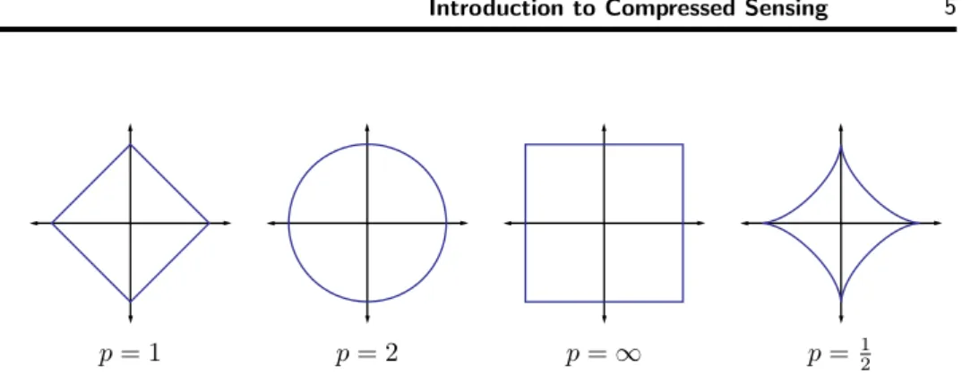
p = 1 p = 2 p = ∞ p =

Figure 1.1

Unit spheres in

for the

norms with

= 1, 2,

quasinorm with

=

.

the linear structure that we often desire, namely that if we add two signals together then we obtain a new, physically meaningful signal. Moreover, vector spaces allow us to apply intuitions and tools from geometry in R

, such as lengths, distances, and angles, to describe and compare signals of interest. This is useful even when our signals live in high-dimensional or infinite-dimensional spaces.

This book assumes that the reader is relatively comfortable with vector spaces.

We now provide only a brief review of some of the key concepts in vector spaces that will be required in developing the CS theory.

1.2.1 Normed vector spaces

Throughout this book, we will treat signals as real-valued functions having domains that are either continuous or discrete, and either infinite or finite. These assumptions will be made clear as necessary in each chapter. We will typically be concerned with normed vector spaces, i.e., vector spaces endowed with a norm.

In the case of a discrete, finite domain, we can view our signals as vectors in an n-dimensional Euclidean space, denoted by R

. When dealing with vectors in R

, we will make frequent use of the `

norms, which are defined for p ∈ [1, ∞]

as

kxk

=





 ( P

i=1

|x

|

)

, p ∈ [1, ∞);

i=1,2,...,n

max |x

|, p = ∞. (1.1) In Euclidean space we can also consider the standard inner product in R

, which we denote

hx, zi = z

x =

n

X

i=1

x

z

. This inner product leads to the `

norm: kxk

= p

hx, xi.

In some contexts it is useful to extend the notion of `

norms to the case

where p < 1. In this case, the “norm” defined in (1.1) fails to satisfy the triangle

inequality, so it is actually a quasinorm. We will also make frequent use of the

notation kxk

:= |supp(x)|, where supp(x) = {i : x

6= 0} denotes the support of

x

A x

A x

x

x x A

x

A x

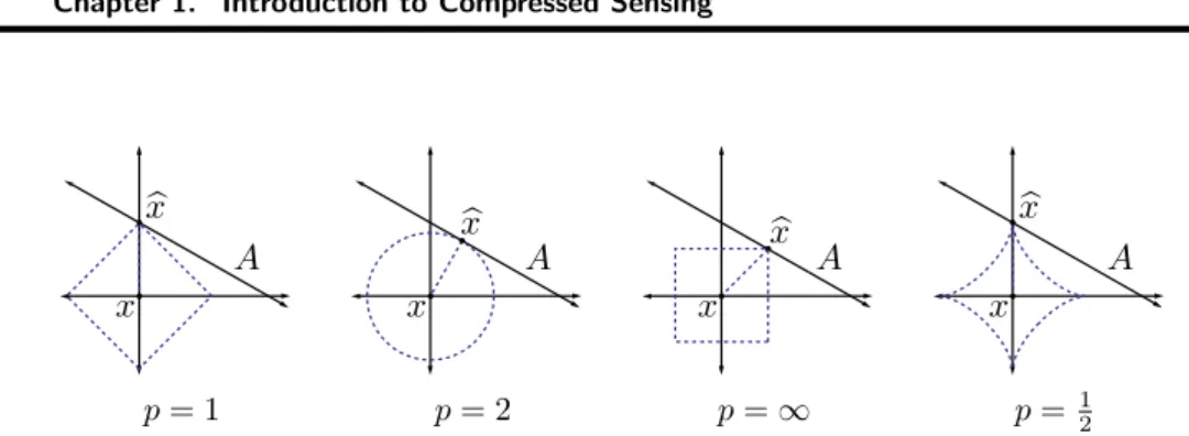
p = 1 p = 2 p = ∞ p =

Figure 1.2

Best approximation of a point in

by a one-dimensional subspace using the

norms for

= 1, 2,

quasinorm with

=

.

x and |supp(x)| denotes the cardinality of supp(x). Note that k·k

is not even a quasinorm, but one can easily show that

p→0

lim kxk

= |supp(x)|,

justifying this choice of notation. The `

(quasi-)norms have notably different properties for different values of p. To illustrate this, in Fig. 1.1 we show the unit sphere, i.e., {x : kxk

= 1}, induced by each of these norms in R

.

We typically use norms as a measure of the strength of a signal, or the size of an error. For example, suppose we are given a signal x ∈ R

and wish to approximate it using a point in a one-dimensional affine space A. If we measure the approximation error using an `

norm, then our task is to find the b x ∈ A that minimizes kx − b xk

. The choice of p will have a significant effect on the properties of the resulting approximation error. An example is illustrated in Fig. 1.2. To compute the closest point in A to x using each `

norm, we can imagine growing an `

sphere centered on x until it intersects with A. This will be the point x b ∈ A that is closest to x in the corresponding `

norm. We observe that larger p tends to spread out the error more evenly among the two coefficients, while smaller p leads to an error that is more unevenly distributed and tends to be sparse. This intuition generalizes to higher dimensions, and plays an important role in the development of CS theory.

1.2.2 Bases and frames

A set {φ

}

is called a basis for R

if the vectors in the set span R

and are linearly independent.

This implies that each vector in the space has a unique representation as a linear combination of these basis vectors. Specifically, for any x ∈ R

, there exist (unique) coefficients {c

}

such that

x =

n

X

i=1

c

φ

.

2 In anyn-dimensional vector space, a basis will always consist of exactlynvectors. Fewer vectors are not sufficient to span the space, while additional vectors are guaranteed to be linearly dependent.

Note that if we let Φ denote the n × n matrix with columns given by φ

and let c denote the length-n vector with entries c

, then we can represent this relation more compactly as

x = Φc.

An important special case of a basis is an orthonormal basis, defined as a set of vectors {φ

}

satisfying

hφ

, φ

i =

( 1, i = j;

0 , i 6= j.

An orthonormal basis has the advantage that the coefficients c can be easily calculated as

c

= hx, φ

i, or

c = Φ

x

in matrix notation. This can easily be verified since the orthonormality of the columns of Φ means that Φ

Φ = I , where I denotes the n × n identity matrix.

It is often useful to generalize the concept of a basis to allow for sets of possibly linearly dependent vectors, resulting in what is known as a frame [48, 55, 65, 163, 164, 182]. More formally, a frame is a set of vectors {φ

}

in R

, d < n corresponding to a matrix Φ ∈ R

, such that for all vectors x ∈ R

,

A kxk

≤ Φ

x

2

2

≤ B kxk

with 0 < A ≤ B < ∞. Note that the condition A > 0 implies that the rows of Φ must be linearly independent. When A is chosen as the largest possible value and B as the smallest for these inequalities to hold, then we call them the (optimal) frame bounds. If A and B can be chosen as A = B, then the frame is called A-tight, and if A = B = 1, then Φ is a Parseval frame. A frame is called equal- norm, if there exists some λ > 0 such that kφ

k

= λ for all i = 1, . . . , n, and it is unit-norm if λ = 1. Note also that while the concept of a frame is very general and can be defined in infinite-dimensional spaces, in the case where Φ is a d × n matrix A and B simply correspond to the smallest and largest eigenvalues of ΦΦ

, respectively.

Frames can provide richer representations of data due to their redundancy [26]:

for a given signal x, there exist infinitely many coefficient vectors c such that x = Φc. In order to obtain a set of feasible coefficients we exploit the dual frame Φ. Specifically, any frame satisfying e

Φe Φ

= ΦΦ e

= I

is called an (alternate) dual frame. The particular choice ˜ Φ = (ΦΦ

)

Φ is

referred to as the canonical dual frame. It is also known as the Moore-Penrose

pseudoinverse. Note that since A > 0 requires Φ to have linearly independent rows, this also ensures that ΦΦ

is invertible, so that ˜ Φ is well-defined. Thus, one way to obtain a set of feasible coefficients is via

c

= (ΦΦ

)

Φx.

One can show that this sequence is the smallest coefficient sequence in `

norm, i.e., kc

k

≤ kck

for all c such that x = Φc.

Finally, note that in the sparse approximation literature, it is also common for a basis or frame to be referred to as a dictionary or overcomplete dictionary respectively, with the dictionary elements being called atoms.

1.3 Low-Dimensional Signal Models

At its core, signal processing is concerned with efficient algorithms for acquiring, processing, and extracting information from different types of signals or data.

In order to design such algorithms for a particular problem, we must have accu- rate models for the signals of interest. These can take the form of generative models, deterministic classes, or probabilistic Bayesian models. In general, mod- els are useful for incorporating a priori knowledge to help distinguish classes of interesting or probable signals from uninteresting or improbable signals. This can help in efficiently and accurately acquiring, processing, compressing, and communicating data and information.

As noted in the introduction, much of classical signal processing is based on the notion that signals can be modeled as vectors living in an appropriate vector space (or subspace). To a large extent, the notion that any possible vector is a valid signal has driven the explosion in the dimensionality of the data we must sample and process. However, such simple linear models often fail to capture much of the structure present in many common classes of signals — while it may be reasonable to model signals as vectors, in many cases not all possible vectors in the space represent valid signals. In response to these challenges, there has been a surge of interest in recent years, across many fields, in a variety of low- dimensional signal models that quantify the notion that the number of degrees of freedom in high-dimensional signals is often quite small compared to their ambient dimensionality.

In this section we provide a brief overview of the most common low-dimensional

structures encountered in the field of CS. We will begin by considering the tradi-

tional sparse models for finite-dimensional signals, and then discuss methods for

generalizing these classes to infinite-dimensional (continuous-time) signals. We

will also briefly discuss low-rank matrix and manifold models and describe some

interesting connections between CS and some other emerging problem areas.

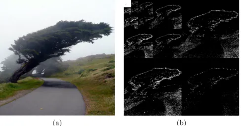
(a) (b)

Figure 1.3

Sparse representation of an image via a multiscale wavelet transform.

(a) Original image. (b) Wavelet representation. Large coefficients are represented by light pixels, while small coefficients are represented by dark pixels. Observe that most of the wavelet coefficients are close to zero.

1.3.1 Sparse models

Signals can often be well-approximated as a linear combination of just a few elements from a known basis or dictionary. When this representation is exact we say that the signal is sparse. Sparse signal models provide a mathematical framework for capturing the fact that in many cases these high-dimensional signals contain relatively little information compared to their ambient dimension.

Sparsity can be thought of as one incarnation of Occam’s razor — when faced with many possible ways to represent a signal, the simplest choice is the best one.

Sparsity and nonlinear approximation

Mathematically, we say that a signal x is k-sparse when it has at most k nonzeros, i.e., kxk

≤ k. We let

Σ

= {x : kxk

≤ k}

denote the set of all k-sparse signals. Typically, we will be dealing with signals that are not themselves sparse, but which admit a sparse representation in some basis Φ. In this case we will still refer to x as being k -sparse, with the under- standing that we can express x as x = Φc where kck

≤ k.

Sparsity has long been exploited in signal processing and approximation the-

ory for tasks such as compression [77, 199, 215] and denoising [80], and in statis-

tics and learning theory as a method for avoiding overfitting [234]. Sparsity

also figures prominently in the theory of statistical estimation and model selec-

tion [139, 218], in the study of the human visual system [196], and has been

exploited heavily in image processing tasks, since the multiscale wavelet trans-

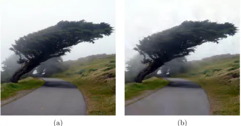
(a) (b)

Figure 1.4

Sparse approximation of a natural image. (a) Original image.

(b) Approximation of image obtained by keeping only the largest 10% of the wavelet coefficients.

form [182] provides nearly sparse representations for natural images. An example is shown in Fig. 1.3.

As a traditional application of sparse models, we consider the problems of image compression and image denoising. Most natural images are characterized by large smooth or textured regions and relatively few sharp edges. Signals with this structure are known to be very nearly sparse when represented using a mul- tiscale wavelet transform [182]. The wavelet transform consists of recursively dividing the image into its low- and high-frequency components. The lowest fre- quency components provide a coarse scale approximation of the image, while the higher frequency components fill in the detail and resolve edges. What we see when we compute a wavelet transform of a typical natural image, as shown in Fig. 1.3, is that most coefficients are very small. Hence, we can obtain a good approximation of the signal by setting the small coefficients to zero, or thresh- olding the coefficients, to obtain a k-sparse representation. When measuring the approximation error using an `

norm, this procedure yields the best k-term approximation of the original signal, i.e., the best approximation of the signal using only k basis elements.

Figure 1.4 shows an example of such an image and its best k-term approxima- tion. This is the heart of nonlinear approximation [77] — nonlinear because the choice of which coefficients to keep in the approximation depends on the signal itself. Similarly, given the knowledge that natural images have approximately sparse wavelet transforms, this same thresholding operation serves as an effec-

3 Thresholding yields the bestk-term approximation of a signal with respect to an orthonormal basis. When redundant frames are used, we must rely on sparse approximation algorithms like those described in Section 1.6 [106, 182].

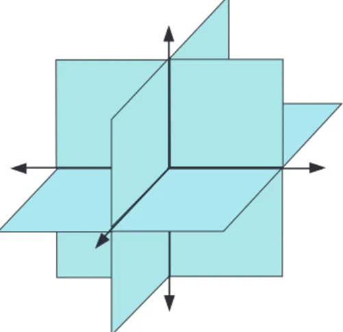
Figure 1.5

Union of subspaces defined by Σ

, i.e., the set of all 2-sparse signals in

.

tive method for rejecting certain common types of noise, which typically do not have sparse wavelet transforms [80].

Geometry of sparse signals

Sparsity is a highly nonlinear model, since the choice of which dictionary elements are used can change from signal to signal [77]. This can be seen by observing that given a pair of k-sparse signals, a linear combination of the two signals will in general no longer be k sparse, since their supports may not coincide. That is, for any x, z ∈ Σ

, we do not necessarily have that x + z ∈ Σ

(although we do have that x + z ∈ Σ

). This is illustrated in Fig. 1.5, which shows Σ

embedded in R

, i.e., the set of all 2-sparse signals in R

.

The set of sparse signals Σ

does not form a linear space. Instead it consists of the union of all possible

canonical subspaces.

In Fig. 1.5 we have only

3 2

= 3 possible subspaces, but for larger values of n and k we must consider a potentially huge number of subspaces. This will have significant algorithmic consequences in the development of the algorithms for sparse approximation and sparse recovery described in Sections 1.5 and 1.6.

Compressible signals

An important point in practice is that few real-world signals are truly sparse;

rather they are compressible, meaning that they can be well-approximated by a sparse signal. Such signals have been termed compressible, approximately sparse, or relatively sparse in various contexts. Compressible signals are well approxi- mated by sparse signals in the same way that signals living close to a subspace

4 Union of subspaces

are well approximated by the first few principal components [139]. In fact, we can quantify the compressibility by calculating the error incurred by approximating a signal x by some b x ∈ Σ

:

σ

( x )

= min

bx∈Σk

kx − b xk

. (1.2)

If x ∈ Σ

, then clearly σ

(x)

= 0 for any p. Moreover, one can easily show that the thresholding strategy described above (keeping only the k largest coefficients) results in the optimal approximation as measured by (1.2) for all `

norms [77].

Another way to think about compressible signals is to consider the rate of decay of their coefficients. For many important classes of signals there exist bases such that the coefficients obey a power law decay, in which case the signals are highly compressible. Specifically, if x = Φc and we sort the coefficients c

such that |c

| ≥ |c

| ≥ · · · ≥ |c

|, then we say that the coefficients obey a power law decay if there exist constants C

, q > 0 such that

|c

| ≤ C

i

.

The larger q is, the faster the magnitudes decay, and the more compressible a signal is. Because the magnitudes of their coefficients decay so rapidly, compress- ible signals can be represented accurately by k n coefficients. Specifically, for such signals there exist constants C

, r > 0 depending only on C

and q such that

σ

(x)

≤ C

k

.

In fact, one can show that σ

(x)

will decay as k

if and only if the sorted coefficients c

decay as i

[77].

1.3.2 Finite unions of subspaces

In certain applications, the signal has a structure that cannot be completely expressed using sparsity alone. For instance, when only certain sparse support patterns are allowable in the signal, it is possible to leverage such constraints to formulate more concise signal models. We give a few representative examples below; see Chapters 2 and 8 for more detail on structured sparsity.

r For piecewise-smooth signals and images, the dominant coefficients in the wavelet transform tend to cluster into a connected rooted subtree inside the wavelet parent-child binary tree [79, 103, 104, 167, 168].

r In applications such as surveillance or neuronal recording, the coefficients might appear clustered together, or spaced apart from each other [49, 50, 147].

See Chapter 11 for more details.

r When multiple sparse signals are recorded simultaneously, their supports

might be correlated according to the properties of the sensing environment [7,

63, 76, 114, 121, 185]. One possible structure leads to the multiple measurement

vector problem; see Section 1.7 for more details.

r In certain cases the small number of components of a sparse signal correspond not to vectors (columns of a matrix Φ), but rather to points known to lie in particular subspaces. If we construct a frame by concatenating bases for such subspaces, the nonzero coefficients of the signal representations form block structures at known locations [27, 112, 114]. See Chapters 3, 11, and 12 for further description and potential applications of this model.

Such examples of additional structure can be captured in terms of restricting the feasible signal supports to a small subset of the possible

selections of nonzero coefficients for a k-sparse signal. These models are often referred to as structured sparsity models [4, 25, 102, 114, 177]. In cases where nonzero coefficients appear in clusters, the structure can be expressed in terms of a sparse union of sub- spaces [102, 114]. Structured sparse and union of subspace models extend the notion of sparsity to a much broader class of signals that can incorporate both finite-dimensional and infinite-dimensional representations.

In order to define these models, recall that for canonically sparse signals, the union Σ

is composed of canonical subspaces U

that are aligned with k out of the n coordinate axes of R

. See, for example, Fig. 1.5, which illustrates this for the case where n = 3 and k = 2. Allowing for more general choices of U

leads to powerful representations that accommodate many interesting signal priors.

Specifically, given the knowledge that x resides in one of M possible subspaces U

, U

, . . . , U

, we have that x lies in the union of M subspaces! [114, 177]:

x ∈ U =

M

[

i=1

U

.

It is important to note that, as in the generic sparse setting, union models are nonlinear: the sum of two signals from a union U is generally no longer in U. This nonlinear behavior of the signal set renders any processing that exploits these models more intricate. Therefore, instead of attempting to treat all unions in a unified way, we focus our attention on some specific classes of union models, in order of complexity.

The simplest class of unions arises when the number of subspaces comprising the union is finite, and each subspace has finite dimensions. We call this setup a finite union of subspaces model. Under the finite-dimensional framework, we revisit the two types of models described above:

r Structured sparse supports: This class consists of sparse vectors that meet

additional restrictions on the support (i.e., the set of indices for the vector’s

nonzero entries). This corresponds to only certain subspaces U

out of the

subspaces present in Σ

being allowed [4].

r Sparse union of subspaces where each subspace U

comprising the union is a direct sum of k low-dimensional subspaces [114].

U

=

k

M

j=1

A

. (1.3)

Here {A

} are a given set of subspaces with dimensions dim(A

) = d

, and i

, i

, . . . , i

select k of these subspaces. Thus, each subspace U

corresponds to a different choice of k out of M subspaces A

that comprise the sum. This framework can model standard sparsity by letting A

be the one-dimensional subspace spanned by the j

canonical vector. It can be shown that this model leads to block sparsity in which certain blocks in a vector are zero, and others are not [112].

These two cases can be combined to allow for only certain sums of k subspaces to be part of the union U . Both models can be leveraged to further reduce sampling rate and allow for CS of a broader class of signals.

1.3.3 Unions of subspaces for analog signal models

One of the primary motivations for CS is to design new sensing systems for acquiring continuous-time, analog signals or images. In contrast, the finite- dimensional sparse model described above inherently assumes that the signal x is discrete. It is sometimes possible to extend this model to continuous-time sig- nals using an intermediate discrete representation. For example, a band-limited, periodic signal can be perfectly represented by a finite-length vector consist- ing of its Nyquist-rate samples. However, it will often be more useful to extend the concept of sparsity to provide union of subspaces models for analog sig- nals [97, 109, 114, 125, 186–188, 239]. Two of the broader frameworks that treat sub-Nyquist sampling of analog signals are Xampling and finite-rate of innova- tion, which are discussed in Chapters 3 and 4, respectively.

In general, when treating unions of subspaces for analog signals there are three main cases to consider, as elaborated further in Chapter 3 [102]:

r finite unions of infinite dimensional spaces;

r infinite unions of finite dimensional spaces;

r infinite unions of infinite dimensional spaces.

In each of the three settings above there is an element that can take on infinite values, which is a result of the fact that we are considering analog signals: either the underlying subspaces are infinite-dimensional, or the number of subspaces is infinite.

There are many well-known examples of analog signals that can be expressed as a union of subspaces. For example, an important signal class corresponding to a finite union of infinite dimensional spaces is the multiband model [109].

In this model, the analog signal consists of a finite sum of bandlimited signals,

where typically the signal components have a relatively small bandwidth but are distributed across a comparatively large frequency range [117, 118, 186, 237, 238].

Sub-Nyquist recovery techniques for this class of signals can be found in [186–

188].

Another example of a signal class that can often be expressed as a union of subspaces is the class of signals having a finite rate of innovation [97, 239].

Depending on the specific structure, this model corresponds to an infinite or finite union of finite dimensional subspaces [19, 125, 126], and describes many common signals having a small number of degrees of freedom. In this case, each subspace corresponds to a certain choice of parameter values, with the set of possible values being infinite dimensional, and thus the number of subspaces spanned by the model being infinite as well. The eventual goal is to exploit the available structure in order to reduce the sampling rate; see Chapters 3 and 4 for more details. As we will see in Chapter 3, by relying on the analog union of subspace model we can design efficient hardware that samples analog signals at sub-Nyquist rates, thus moving the analog CS framework from theory to practice.

1.3.4 Low-rank matrix models

Another model closely related to sparsity is the set of low-rank matrices:

L = {M ∈ R

: rank( M ) ≤ r}.

The set L consists of matrices M such that M = P

k=1

σ

u

v

where σ

, σ

, . . . , σ

≥ 0 are the nonzero singular values, and u

, u

, . . . , u

∈ R

, v

, v

, . . . , v

∈ R

are the corresponding singular vectors. Rather than con- straining the number of elements used to construct the signal, we are constrain- ing the number of nonzero singular values. One can easily observe that the set L has r(n

+ n

− r) degrees of freedom by counting the number of free parameters in the singular value decomposition. For small r this is significantly less than the number of entries in the matrix — n

n

. Low-rank matrices arise in a variety of practical settings. For example, low-rank (Hankel) matrices correspond to low- order linear, time-invariant systems [198]. In many data-embedding problems, such as sensor geolocation, the matrix of pairwise distances will typically have rank 2 or 3 [172, 212]. Finally, approximately low-rank matrices arise naturally in the context of collaborative filtering systems such as the now-famous Netflix rec- ommendation system [132] and the related problem of matrix completion, where a low-rank matrix is recovered from a small sample of its entries [39, 151, 204].

While we do not focus in-depth on matrix completion or the more general prob-

lem of low-rank matrix recovery, we note that many of the concepts and tools

treated in this book are highly relevant to this emerging field, both from a the-

oretical and algorithmic perspective [36, 38, 161, 203].

1.3.5 Manifold and parametric models

Parametric or manifold models form another, more general class of low- dimensional signal models. These models arise in cases where (i) a k-dimensional continuously-valued parameter θ can be identified that carries the relevant infor- mation about a signal and (ii) the signal f (θ) ∈ R

changes as a continuous (typically nonlinear) function of these parameters. Typical examples include a one-dimensional (1-D) signal shifted by an unknown time delay (parameterized by the translation variable), a recording of a speech signal (parameterized by the underlying phonemes being spoken), and an image of a 3-D object at an unknown location captured from an unknown viewing angle (parameterized by the 3-D coordinates of the object and its roll, pitch, and yaw) [90, 176, 240]. In these and many other cases, the signal class forms a nonlinear k-dimensional manifold in R

, i.e.,

M = {f (θ) : θ ∈ Θ},

where Θ is the k-dimensional parameter space. Manifold-based methods for image processing have attracted considerable attention, particularly in the machine learning community. They can be applied to diverse applications includ- ing data visualization, signal classification and detection, parameter estimation, systems control, clustering, and machine learning [14, 15, 58, 61, 89, 193, 217, 240, 244]. Low-dimensional manifolds have also been proposed as approximate mod- els for a number of nonparametric signal classes such as images of human faces and handwritten digits [30, 150, 229].

Manifold models are closely related to all of the models described above.

For example, the set of signals x such that kxk

= k forms a k-dimensional Riemannian manifold. Similarly, the set of n

× n

matrices of rank r forms an r ( n

+ n

− r )-dimensional Riemannian manifold [233].

Furthermore, many manifolds can be equivalently described as an infinite union of subspaces.

A number of the signal models used in this book are closely related to manifold models. For example, the union of subspace models in Chapter 3, the finite rate of innovation models considered in Chapter 4, and the continuum models in Chapter 11 can all be viewed from a manifold perspective. For the most part we will not explicitly exploit this structure in the book. However, low- dimensional manifolds have a close connection to many of the key results in CS.

In particular, many of the randomized sensing matrices used in CS can also be shown to preserve the structure in low-dimensional manifolds [6]. For details and further applications see [6, 71, 72, 101].

5 Note that in the case where we allow signals with sparsity less than or equal tok, or matrices of rank less than or equal tor, these sets fail to satisfy certain technical requirements of a topological manifold (due to the behavior where the sparsity/rank changes). However, the manifold viewpoint can still be useful in this context [68].

1.4 Sensing Matrices

In order to make the discussion more concrete, for the remainder of this chapter we will restrict our attention to the standard finite-dimensional CS model. Specif- ically, given a signal x ∈ R

, we consider measurement systems that acquire m linear measurements. We can represent this process mathematically as

y = Ax, (1.4)

where A is an m × n matrix and y ∈ R

. The matrix A represents a dimen- sionality reduction, i.e., it maps R

, where n is generally large, into R

, where m is typically much smaller than n. Note that in the standard CS framework we assume that the measurements are non-adaptive, meaning that the rows of A are fixed in advance and do not depend on the previously acquired measure- ments. In certain settings adaptive measurement schemes can lead to significant performance gains. See Chapter 6 for further details.

As noted earlier, although the standard CS framework assumes that x is a finite-length vector with a discrete-valued index (such as time or space), in prac- tice we will often be interested in designing measurement systems for acquir- ing continuously-indexed signals such as continuous-time signals or images. It is sometimes possible to extend this model to continuously-indexed signals using an intermediate discrete representation. For a more flexible approach, we refer the reader to Chapters 3 and 4. For now we will simply think of x as a finite- length window of Nyquist-rate samples, and we temporarily ignore the issue of how to directly acquire compressive measurements without first sampling at the Nyquist rate.

There are two main theoretical questions in CS. First, how should we design the sensing matrix A to ensure that it preserves the information in the signal x? Second, how can we recover the original signal x from measurements y? In the case where our data is sparse or compressible, we will see that we can design matrices A with m n that ensure that we will be able to recover the original signal accurately and efficiently using a variety of practical algorithms.

We begin in this section by first addressing the question of how to design the sensing matrix A. Rather than directly proposing a design procedure, we instead consider a number of desirable properties that we might wish A to have.

We then provide some important examples of matrix constructions that satisfy these properties.

1.4.1 Null space conditions

A natural place to begin is by considering the null space of A, denoted N ( A ) = {z : Az = 0}.

If we wish to be able to recover all sparse signals x from the measurements

Ax, then it is immediately clear that for any pair of distinct vectors x, x

∈ Σ

,

we must have Ax 6= Ax

, since otherwise it would be impossible to distinguish x from x

based solely on the measurements y. More formally, by observing that if Ax = Ax

then A ( x − x

) = 0 with x − x

∈ Σ

, we see that A uniquely represents all x ∈ Σ

if and only if N (A) contains no vectors in Σ

. While there are many equivalent ways of characterizing this property, one of the most common is known as the spark [86].

Definition 1.1. The spark of a given matrix A is the smallest number of columns of A that are linearly dependent.

This definition allows us to pose the following straightforward guarantee.

Theorem 1.1 (Corollary 1 of [86]). For any vector y ∈ R

, there exists at most one signal x ∈ Σ

such that y = Ax if and only if spark(A) > 2k.

Proof. We first assume that, for any y ∈ R

, there exists at most one signal x ∈ Σ

such that y = Ax . Now suppose for the sake of a contradiction that spark(A) ≤ 2k. This means that there exists some set of at most 2k columns that are linearly independent, which in turn implies that there exists an h ∈ N (A) such that h ∈ Σ

. In this case, since h ∈ Σ

we can write h = x − x

, where x, x

∈ Σ

. Thus, since h ∈ N (A) we have that A(x − x

) = 0 and hence Ax = Ax

. But this contradicts our assumption that there exists at most one signal x ∈ Σ

such that y = Ax. Therefore, we must have that spark(A) > 2k.

Now suppose that spark( A ) > 2 k . Assume that for some y there exist x, x

∈ Σ

such that y = Ax = Ax

. We therefore have that A(x − x

) = 0. Letting h = x − x

, we can write this as Ah = 0. Since spark(A) > 2k, all sets of up to 2k columns of A are linearly independent, and therefore h = 0. This in turn implies x = x

, proving the theorem.

It is easy to see that spark( A ) ∈ [2 , m + 1]. Therefore, Theorem 1.1 yields the requirement m ≥ 2k.

When dealing with exactly sparse vectors, the spark provides a complete char-

acterization of when sparse recovery is possible. However, when dealing with

approximately sparse signals we must consider somewhat more restrictive condi-

tions on the null space of A [57]. Roughly speaking, we must also ensure that

N (A) does not contain any vectors that are too compressible in addition to vec-

tors that are sparse. In order to state the formal definition we define the following

notation that will prove to be useful throughout much of this book. Suppose that

Λ ⊂ {1, 2, . . . , n} is a subset of indices and let Λ

= {1, 2, . . . , n}\Λ. By x

we

typically mean the length n vector obtained by setting the entries of x indexed

by Λ

to zero. Similarly, by A

we typically mean the m × n matrix obtained by setting the columns of A indexed by Λ

to zero.

Definition 1.2. A matrix A satisfies the null space property (NSP) of order k if there exists a constant C > 0 such that,

kh

k

≤ C kh

k

√ k (1.5)

holds for all h ∈ N (A) and for all Λ such that |Λ| ≤ k.

The NSP quantifies the notion that vectors in the null space of A should not be too concentrated on a small subset of indices. For example, if a vector h is exactly k-sparse, then there exists a Λ such that kh

k

= 0 and hence (1.5) implies that h

= 0 as well. Thus, if a matrix A satisfies the NSP then the only k-sparse vector in N (A) is h = 0.

To fully illustrate the implications of the NSP in the context of sparse recovery, we now briefly discuss how we will measure the performance of sparse recovery algorithms when dealing with general non-sparse x . Towards this end, let ∆ : R

→ R

represent our specific recovery method. We will focus primarily on guarantees of the form

k∆(Ax) − xk

≤ C σ

(x)

√ k (1.6)

for all x, where σ

(x)

is as defined in (1.2). This guarantees exact recovery of all possible k -sparse signals, but also ensures a degree of robustness to non-sparse signals that directly depends on how well the signals are approximated by k- sparse vectors. Such guarantees are called instance-optimal since they guarantee optimal performance for each instance of x [57]. This distinguishes them from guarantees that only hold for some subset of possible signals, such as sparse or compressible signals — the quality of the guarantee adapts to the particular choice of x. These are also commonly referred to as uniform guarantees since they hold uniformly for all x .

Our choice of norms in (1.6) is somewhat arbitrary. We could easily measure the reconstruction error using other `

norms. The choice of p, however, will limit what kinds of guarantees are possible, and will also potentially lead to alternative formulations of the NSP. See, for instance, [57]. Moreover, the form of the right-hand-side of (1.6) might seem somewhat unusual in that we measure the approximation error as σ

(x)

/ √

k rather than simply something like σ

(x)

. However, we will see in Section 1.5.3 that such a guarantee is actually not possible

6 We note that this notation will occasionally be abused to refer to the length |Λ| vector obtained by keeping only the entries corresponding to Λ or them× |Λ|matrix obtained by only keeping the columns corresponding to Λ respectively. The usage should be clear from the context, but in most cases there is no substantive difference between the two.

without taking a prohibitively large number of measurements, and that (1.6) represents the best possible guarantee we can hope to obtain.

We will see in Section 1.5 (Theorem 1.8) that the NSP of order 2k is sufficient to establish a guarantee of the form (1.6) for a practical recovery algorithm (`

minimization). Moreover, the following adaptation of a theorem in [57] demon- strates that if there exists any recovery algorithm satisfying (1.6), then A must necessarily satisfy the NSP of order 2k.

Theorem 1.2 (Theorem 3.2 of [57]). Let A : R

→ R

denote a sensing matrix and ∆ : R

→ R

denote an arbitrary recovery algorithm. If the pair (A, ∆) satisfies (1.6) then A satisfies the NSP of order 2k.

Proof. Suppose h ∈ N (A) and let Λ be the indices corresponding to the 2k largest entries of h. We next split Λ into Λ

and Λ

, where |Λ

| = |Λ

| = k. Set x = h

+ h

and x

= −h

, so that h = x − x

. Since by construction x

∈ Σ

, we can apply (1.6) to obtain x

= ∆(Ax

). Moreover, since h ∈ N (A), we have

Ah = A (x − x

) = 0

so that Ax

= Ax. Thus, x

= ∆(Ax). Finally, we have that kh

k

≤ khk

= kx − x

k

= kx − ∆( Ax )k

≤ C σ

(x)

√ k = √

2 C kh

k

√ 2k , where the last inequality follows from (1.6).

1.4.2 The restricted isometry property

While the NSP is both necessary and sufficient for establishing guarantees of the form (1.6), these guarantees do not account for noise. When the measure- ments are contaminated with noise or have been corrupted by some error such as quantization, it will be useful to consider somewhat stronger conditions. In [43], Cand` es and Tao introduced the following isometry condition on matrices A and established its important role in CS.

Definition 1.3. A matrix A satisfies the restricted isometry property (RIP) of order k if there exists a δ

∈ (0 , 1) such that

(1 − δ

) kxk

≤ kAxk

≤ (1 + δ

) kxk

, (1.7) holds for all x ∈ Σ

.

If a matrix A satisfies the RIP of order 2k, then we can interpret (1.7) as

saying that A approximately preserves the distance between any pair of k -sparse

vectors. This will clearly have fundamental implications concerning robustness

to noise. Moreover, the potential applications of such stable embeddings range

far beyond acquisition for the sole purpose of signal recovery. See Chapter 10 for examples of additional applications.

It is important to note that while in our definition of the RIP we assume bounds that are symmetric about 1, this is merely for notational convenience.

In practice, one could instead consider arbitrary bounds α kxk

≤ kAxk

≤ β kxk

where 0 < α ≤ β < ∞. Given any such bounds, one can always scale A so that it satisfies the symmetric bound about 1 in (1.7). Specifically, multiplying A by p

2/(β + α) will result in an A e that satisfies (1.7) with constant δ

= (β − α ) / ( β + α ). While we will not explicitly show this, one can check that all of the theorems in this chapter based on the assumption that A satisfies the RIP actually hold as long as there exists some scaling of A that satisfies the RIP.

Thus, since we can always scale A to satisfy (1.7), we lose nothing by restricting our attention to this simpler bound.

Note also that if A satisfies the RIP of order k with constant δ

, then for any k

< k we automatically have that A satisfies the RIP of order k

with constant δ

≤ δ

. Moreover, in [190] it is shown that if A satisfies the RIP of order k with a sufficiently small constant, then it will also automatically satisfy the RIP of order γk for certain γ, albeit with a somewhat worse constant.

Lemma 1.1 (Corollary 3.4 of [190]). Suppose that A satisfies the RIP of order k with constant δ

. Let γ be a positive integer. Then A satisfies the RIP of order k

= γ

2

with constant δ

< γ · δ

, where b·c denotes the floor operator.

This lemma is trivial for γ = 1, 2, but for γ ≥ 3 (and k ≥ 4) this allows us to extend from RIP of order k to higher orders. Note however, that δ

must be sufficiently small in order for the resulting bound to be useful.

The RIP and stability

We will see in Sections 1.5 and 1.6 that if a matrix A satisfies the RIP, then this is sufficient for a variety of algorithms to be able to successfully recover a sparse signal from noisy measurements. First, however, we will take a closer look at whether the RIP is actually necessary. It should be clear that the lower bound in the RIP is a necessary condition if we wish to be able to recover all sparse signals x from the measurements Ax for the same reasons that the NSP is necessary. We can say even more about the necessity of the RIP by considering the following notion of stability [67].

Definition 1.4. Let A : R

→ R

denote a sensing matrix and ∆ : R

→ R

denote a recovery algorithm. We say that the pair (A, ∆) is C-stable if for any x ∈ Σ

and any e ∈ R

we have that

k∆ (Ax + e) − xk

≤ C kek

.

This definition simply says that if we add a small amount of noise to the measurements, then the impact of this on the recovered signal should not be arbitrarily large. Theorem 1.3 below demonstrates that the existence of any decoding algorithm (potentially impractical) that can stably recover from noisy measurements requires that A satisfy the lower bound of (1.7) with a constant determined by C.

Theorem 1.3 (Theorem 3.1 of [67]). If the pair (A, ∆) is C-stable, then 1

C kxk

≤ kAxk

(1.8)

for all x ∈ Σ

.

Proof. Pick any x, z ∈ Σ

. Define e

= A(z − x)

2 and e

= A(x − z)

2 ,

and note that

Ax + e

= Az + e

= A(x + z)

2 .

Let b x = ∆(Ax + e

) = ∆(Az + e

). From the triangle inequality and the defini- tion of C -stability, we have that

kx − zk

= kx − b x + b x − zk

≤ kx − b xk

+ k x b − zk

≤ C ke

k

+ C ke

k

= C kAx − Azk

. Since this holds for any x, z ∈ Σ

, the result follows.

Note that as C → 1, we have that A must satisfy the lower bound of (1.7) with δ

= 1 − 1/C

→ 0. Thus, if we desire to reduce the impact of noise in our recovered signal then we must adjust A so that it satisfies the lower bound of (1.7) with a tighter constant.

One might respond to this result by arguing that since the upper bound is not necessary, we can avoid redesigning A simply by rescaling A so that as long as A satisfies the RIP with δ

< 1, the rescaled version αA will satisfy (1.8) for any constant C. In settings where the size of the noise is independent of our choice of A, this is a valid point — by scaling A we are essentially adjusting the gain on the “signal” part of our measurements, and if increasing this gain does not impact the noise, then we can achieve arbitrarily high signal-to-noise ratios, so that eventually the noise is negligible compared to the signal.

However, in practice we will typically not be able to rescale A to be arbitrarily

large. Moreover, in many practical settings the noise is not independent of A .

For example, consider the case where the noise vector e represents quantization

noise produced by a finite dynamic range quantizer with B bits. Suppose the

measurements lie in the interval [−T, T ], and we have adjusted the quantizer to capture this range. If we rescale A by α, then the measurements now lie between [−αT, αT ], and we must scale the dynamic range of our quantizer by α.

In this case the resulting quantization error is simply αe, and we have achieved no reduction in the reconstruction error.

Measurement bounds

We can also consider how many measurements are necessary to achieve the RIP.

If we ignore the impact of δ and focus only on the dimensions of the problem (n, m, and k) then we can establish a simple lower bound, which is proven in Section A.1.

Theorem 1.4 (Theorem 3.5 of [67]). Let A be an m × n matrix that satisfies the RIP of order 2k with constant δ ∈ (0,

]. Then

m ≥ Ck log n k

where C = 1/2 log( √

24 + 1) ≈ 0.28.

Note that the restriction to δ ≤

is arbitrary and is made merely for con- venience — minor modifications to the argument establish bounds for δ ≤ δ

for any δ

< 1. Moreover, although we have made no effort to optimize the constants, it is worth noting that they are already quite reasonable.

While the proof is somewhat less direct, one can establish a similar result (in terms of its dependence on n and k) by examining the Gelfand width of the `

ball [124]. However, both this result and Theorem 1.4 fail to capture the precise dependence of m on the desired RIP constant δ . In order to quantify this dependence, we can exploit recent results concerning the Johnson-Lindenstrauss lemma, which relates to embeddings of finite sets of points in low-dimensional spaces [158]. Specifically, it is shown in [156] that if we are given a point cloud with p points and wish to embed these points in R

such that the squared `

distance between any pair of points is preserved up to a factor of 1 ± , then we must have that

m ≥ c

log( p )

, where c

> 0 is a constant.

The Johnson-Lindenstrauss lemma is closely related to the RIP. In [5] it is

shown that any procedure that can be used for generating a linear, distance-

preserving embedding for a point cloud can also be used to construct a matrix

that satisfies the RIP. Moreover, in [165] it is shown that if a matrix A satisfies

the RIP of order k = c

log(p) with constant δ, then A can be used to construct

a distance-preserving embedding for p points with = δ/4. Combining these we

obtain

m ≥ c

log(p)

= 16c

k c

δ

.

Thus, for very small δ the number of measurements required to ensure that A sat- isfies the RIP of order k will be proportional to k/δ

, which may be significantly higher than k log(n/k). See [165] for further details.

The relationship between the RIP and the NSP

Finally, we will now show that if a matrix satisfies the RIP, then it also satisfies the NSP. Thus, the RIP is strictly stronger than the NSP.

Theorem 1.5. Suppose that A satisfies the RIP of order 2k with δ

< √ 2 − 1.

Then A satisfies the NSP of order 2k with constant C =

√ 2δ

1 − (1 + √ 2)δ

.

The proof of this theorem involves two useful lemmas. The first of these follows directly from standard norm inequality by relating a k-sparse vector to a vector in R

. We include a simple proof for the sake of completeness.

Lemma 1.2. Suppose u ∈ Σ

. Then kuk

√ k ≤ kuk

≤ √

k kuk

.

Proof. For any u , kuk

= |hu, sgn( u )i|. By applying the Cauchy-Schwarz inequal- ity we obtain kuk

≤ kuk

ksgn(u)k

. The lower bound follows since sgn(u) has exactly k nonzero entries all equal to ±1 (since u ∈ Σ

) and thus ksgn(u)k

= √

k.

The upper bound is obtained by observing that each of the k nonzero entries of u can be upper bounded by kuk

.

Below we state the second key lemma that we will need in order to prove Theorem 1.5. This result is a general result which holds for arbitrary h, not just vectors h ∈ N ( A ). It should be clear that when we do have h ∈ N ( A ), the argument could be simplified considerably. However, this lemma will prove immensely useful when we turn to the problem of sparse recovery from noisy measurements in Section 1.5, and thus we establish it now in its full generality.

The intuition behind this bound will become more clear after reading Section 1.5.

We state the lemma here, which is proven in Section A.2.

Lemma 1.3. Suppose that A satisfies the RIP of order 2k, and let h ∈ R

, h 6= 0

be arbitrary. Let Λ

be any subset of {1 , 2 , . . . , n} such that |Λ

| ≤ k . Define Λ

as the index set corresponding to the k entries of h

with largest magnitude,

and set Λ = Λ

∪ Λ

. Then kh

k

≤ α

h

√ k + β |hAh

, Ahi|

kh

k

, where

α =

√ 2δ

1 − δ

, β = 1 1 − δ

.

Again, note that Lemma 1.3 holds for arbitrary h. In order to prove Theo- rem 1.5, we merely need to apply Lemma 1.3 to the case where h ∈ N (A).

Proof of Theorem 1.5. Suppose that h ∈ N (A). It is sufficient to show that kh

k

≤ C kh

k

√ k (1.9)

holds for the case where Λ is the index set corresponding to the 2k largest entries of h. Thus, we can take Λ

to be the index set corresponding to the k largest entries of h and apply Lemma 1.3.

The second term in Lemma 1.3 vanishes since Ah = 0, and thus we have kh

k

≤ α

h

√ k . Using Lemma 1.2,

h

= kh

k

+ kh

k

≤ √

k kh

k

+ kh

k

resulting in

kh

k

≤ α

kh

k

+ kh

k

√ k

.

Since kh

k

≤ kh

k

, we have that

(1 − α) kh

k

≤ α kh

k

√ k . The assumption δ

< √

2 − 1 ensures that α < 1, and thus we may divide by 1 − α without changing the direction of the inequality to establish (1.9) with constant

C = α 1 − α =

√ 2δ

1 − (1 + √ 2)δ

,

as desired.

1.4.3 Coherence

While the spark, NSP, and RIP all provide guarantees for the recovery of k-sparse

signals, verifying that a general matrix A satisfies any of these properties has a

combinatorial computational complexity, since in each case one must essentially