Robust Adaptive Model Predictive Control of Quadrotors

(1)

Research Collection

Master Thesis

Robust Adaptive Model Predictive Control of Quadrotors

Author(s):

Didier, Alexandre Publication Date:

2020-08

Permanent Link:

https://doi.org/10.3929/ethz-b-000455248

Rights / License:

In Copyright - Non-Commercial Use Permitted

This page was generated automatically upon download from the ETH Zurich Research Collection. For more information please consult the Terms of use.

ETH Library

(2)

Robust Adaptive Model

Predictive Control of Quadrotors

Master’s Thesis

Automatic Control Laboratory

Swiss Federal Institute of Technology (ETH) Zurich

Supervision Anil Parsi Jeremy Coulson Prof. Dr. Roy Smith

August 2020

(3)

(4)

Abstract

Robust Adaptive Model Predictive Control is a novel control method that combines robustness guarantees with respect to unknown parameters and bounded disturbances into a Model Predictive Control scheme. Given prior information on the parameters, a set of possible parameters is improved online using Set-Membership Estimation while state and input constraint satisfaction is guaranteed robustly. In this thesis, we compare three Robust Adaptive Model Predictive Control methods based on their performance, conservatism and computational efficiency. We then run simulations of a quadrotor flight with a direct and decoupled control architecture in different scenarios. These scenarios include an unknown mass of the quadrotor as a package delivery scenario, wind as a bounded disturbance or constant force acting on the quadrotor, single rotor failure and all rotor efficiency drop as a power delivery problem. Lastly, we test Robust Adaptive Model Predictive Control on a real quadrotor.

Keywords: Robust Control, Adaptive Control, Model Predictive Control, Quadrotors.

i

(5)

(6)

Chapter 1 Introduction

Model Predictive Control is an optimisation based control scheme, which guarantees state and input constraint satisfaction at every time step for a discrete time, nominal system. Robust Model Predictive Control integrates robustness guarantees with respect to bounded disturbances and parametric uncertainties in the dynamics into the optimisation problem. In this thesis, we compare three different methods of Robust Adaptive Model Predictive Control (RAMPC), as seen in [1], [2]

and [3]. RAMPC is a novel control method, which combines the robustness guarantees with respect to uncertain parameters and bounded disturbances with online identification of the uncertain parameter in order to improve performance. The novel RAMPC schemes have only been applied to theoretical models and no examples with practical problems like noise were considered. The goal of this thesis is to implement RAMPC on a real quadrotor in order to robustly guarantee a safe flight while achieving good performance.

As an identification method, Set-Membership estimation is used, which intersects the current set of estimates of the parameters with the possible parameters given the system evolution at every time step. This method guarantees that the real parameter will always be within the set of estimates, if it is contained in the prior set of estimates. As this method guarantees consistency for the parameter estimation, it is well suited to give robustness guarantees with respect to this parameter. The three RAMPC methods we consider have different approaches in order to guarantee that state and input constraints on the system will not be violated. As they all vary in terms of conservatism and computational efficiency, we will compare the three methods in a quadrotor flight simulation.

Additionally, we propose solutions to practical problems, which may arise in the application of these control schemes, notably a steady-state input depending on the uncertain parameter and measurement noise. We give both theoretical guarantees which allow to resolve these issues, as well as heuristics which showed good performance during a practical implementation.

In order to show the effectiveness of RAMPC, we test it in different scenarios on the quadrotor. The first scenario, which is used to compare all three methods involves an uncertain quadrotor mass as part of a package delivery scenario. If the mass of the package the drone is delivering is unknown, it may lead to an unsafe flight resulting in a crash of the quadrotor. We thus compare how well RAMPC can cope with such an uncertainty. An uncertain mass is presumed in all experiments. In a second scenario, an unknown wind force is acting on the quadrotor. Wind is a common factor during an outdoors quadrotor flight and has been considered in papers such as [4] and [5]. Finally we consider a loss of efficiency in a single rotor as a failure as well as a loss of efficiency in all rotors as a power delivery problem, as seen in [6] and [7]. These scenarios are evaluated for a direct thrust control of the quadrotor and some on a decoupled control method and are then implemented on a real quadrotor.

The report is structured as follows. Chapter 2 contains a description of the three RAMPC methods we compare including a description of the Set-Membership estimation and a discussion on practical

1

(9)

implementation issues and their solutions. In Chapter 3, we show the results of simulations of different quadrotor flight scenarios and in Chapter 4 we discuss the results of the tests on the real quadrotor.

Notation.The set of integers t1, . . . , nu is given as Nⁿ1, the set of positive reals is R°0 and the n-dimensional set of reals is Rⁿ. A positive semi-definite matrix A fulfils A © 0 and A © B is equivalent toA´B ©0, whereas a matrix whose entries are all non-negative is denoted asA•0.

Thei-th row of the matrixAis given asrAsⁱand thei-th entry of the vectorbasrbsⁱ. The diagonal matrix with entriesa, b, c on its main diagonal is denoted asA“diagpa, b, cqand the convex hull of a set A is defined as copAq. The identity matrix is denoted as I and 1is the vector of ones.

The Euclidean norm ofb is is given byÎbÎ andÎxÎ²A“x^TAx.A‘B denotes the Minkowski set addition.

(10)

Chapter 2 Robust Adaptive Model Predictive Control

In this chapter, three different, novel methods of Robust Adaptive Model Predictive Control are presented and compared with respect to theoretical guarantees, conservatism and performance.

Robust Adaptive Model Predictive Control aims to achieve good performance by using online identification of uncertain parameters while integrating robustness guarantees with respect to these bounded parametric uncertainties and a bounded disturbance into the Model Predictive Control scheme. Firstly a description of how these different methods operate in general is given, by making use of the notation in [1], followed by a detailed description of each method.

2.1 Problem Formulation

Consider linear, discrete time, parameter dependent dynamics with an additive disturbance xk`1“Ap◊qxk`Bp◊quk`wk, (2.1) with the state vectorxkPRⁿ, the disturbancewk PRⁿ, the input vectorukPR^m and the uncertain parameter◊PR^p, whose true value is ◊“◊^˚.

Assumption 1.

1. The disturbance wk is bounded by a convex polytope

wkPW“ twPRⁿ|Hww§hwu, (2.2) withHwPRⁿ^w^ˆⁿ andhwPRⁿ^w.

2. The system matrices Ap◊q and Bp◊q depend affinely on the parameter vector ◊ P R^p, such that

pAp◊q, Bp◊qq “ pA0, B0q ` ÿp

i“1pAi, Biqr◊sⁱ. (2.3) 3. The uncertain parameters◊ are bounded in a convex polytope

◊P 0“ t◊PR^p|H◊◊§h◊u, (2.4) which is known and contains the true parameter vector◊^˚, which is unknown.

3

(11)

The states and inputs are constrained using polytopic state and input constraints

pxk, ukq PZ“ tpx, uq PRⁿˆR^m|F x`Gu§1u, (2.5) withFPRⁿ^z^ˆn andGPRⁿ^z^ˆm.

2.2 Set-Membership Identification

Set-Membership Identification, as presented e.g. in [1], is a parameter identification method, which recursively updates a set of possible parameters that is guaranteed to contain the true parameter.

Given state measurements, the previous input and the bounded disturbance set W, the goal is to identify the uncertain parameter vector ◊ online in order to achieve a better performance as our estimate improves. The Robust Adaptive Model Predictive Control methods presented in [1], [2] and [3] make use of Set-Membership Identification in order to guarantee robustness. The identification method relies on a prior known uncertainty set , which contains the true parameter

◊^˚ and recursively updates the set of parameter estimates while guaranteeing consistency, i.e. the true parameter◊^˚P k,@k•0.

In order to compute this recursive update, the following helper functions are introduced:

Dk“Dpxk, ukq “ rA1xk`B1uk, A2xk`B2uk, . . . , Apxk`Bpuksand (2.6) dk “dpxk, xk´1, uk´1q “A₀xk´1`B₀uk´1´xk, (2.7) which are affine in pxk, ukq.

At every time stepk, the set of possible parameters that explains how the system evolved given the unknown, bounded disturbance can now be computed. This set of parameters k, called the non-falsified parameter set, is given as

k“ t◊PR^p|xk´ pAp◊qxk´1`Bp◊quk´1q PWu

“ t◊PR^p|Hwpxk´ pAp◊qxk´1`Bp◊quk´1qq§hwu (2.8)

“ t◊PR^p| ´HwDk´1◊§hw`Hwdku. The recursive update is then given by

k “ ^k´1X ^k, (2.9)

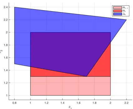
as illustrated in Figure 2.1.

This identification scheme leads to a consistent method for the parameter estimation and k, as the intersection of two convex polytopes remains a convex polytope.

Lemma 1. ( [1])

The set k is a convex, polytopic set explicitly given in half-space form

k “ t◊PR^p|H◊k◊§h◊ku, (2.10) withH◊k PRⁿ^◊^ˆ^p andh◊kPRⁿ^◊,@kPN. Furthermore ◊^˚P ^k and k`1Ñ ^k,@kPN.

It should be noted that by recursively taking intersections of past parameter sets, the complexity of this set and therefore the RAMPC scheme will increase at potentially every time step. Instead, the matrixH◊k can be set constant asH◊ and the vectorh◊k can be updated at every time step.

This leads to a polytope where the directions of the facets are fixed and only their position in the parameter space is updated. In order to guarantee consistency,h◊k needs to be chosen in a way such that

k Ö ^k´1X ^k. (2.11)

(12)

0.8 1 1.2 1.4 1.6 1.8 2 2.2 1

1 1.2 1.4 1.6 1.8 2 2.2 2.4

2

k-1 k k

Figure 2.1: Illustration of Set-Membership Identification. At every time step k, the new set of estimates k is computed through the intersection of the previous set of estimates k´1 and the non-falsified parameter set k.

This can be achieved by solving the following linear program:

hPRⁿ^◊,minPRⁿ^◊^ˆpw1^Th s.t. „

H◊

´HwDk

⇢

“H◊, (2.12)

„ h◊k

hw`Hwdk`1

⇢

§h,

•0,

withpw“n◊`nw. The update (2.11) is illustrated in Figure 2.2. The LP (2.12) follows from the following Lemma from [8].

Lemma 2. ( [8])

Let P1 “ txPRⁿ|H₁x§h₁u andP2 “ txPRⁿ|H₂x§h₂u, withH₁ PRⁿ¹^ˆⁿ, H₂ PRⁿ²^ˆⁿ, f₁P Rⁿ¹ andf2PRⁿ². ThenP1ÑP2 if and only if there exists PRⁿ²^ˆⁿ¹ such that

H₁“H₂,

h1§h2, (2.13)

•0.

Proof. Assume P1ÑP2. Then, by denoting the i-th row ofH2 asrH2sⁱ, it holds @ithat

µi“maxrH2sⁱx (2.14)

s.t.H₁x§h₁.

(13)

whereµi§rh2sⁱ. The dual of the LP (2.14) is given by µi“ min

⁄PR^1ˆn¹⁄h₁

s.t.⁄H₁“ rH₂sⁱ, (2.15)

⁄•0.

The matrix in (2.13) can be constructed by setting thei-th row of to ⁄i. Conversly, assume that exists such that (2.13) is satisfied, then@xPP1it holds that

H₂x“ H₁x§ h₁§h₂.

0.8 1 1.2 1.4 1.6 1.8 2 2.2

1 1

1.2 1.4 1.6 1.8 2 2.2 2.4

2

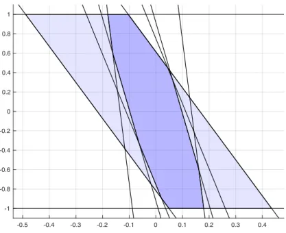
Figure 2.2: Illustration of bounded complexity Set-Membership Identification. The set of estimates

k has a fixed number of hyperplanes which are moved along their normal according to (2.12).

2.3 Tube Model Predictive Control

In order to guarantee robustness with respect to the bounded disturbancewk and the uncertain parameters◊, a state tubetXl|kulPN^N0 is introduced at time step k for the predicted time stepsl.

This tube consists ofN`1predicted polytopesXl|kÄRⁿ in the state space at time stepk, where N is the time horizon of the RAMPC scheme. If at each predicted time stepl|k, it is ensured that the states are inside of the polytopeXl|k for allwPWand◊P ^k, then robustness is guaranteed if the states inside of these polytopes do not violate the state constraints and the computed inputs do not violate the input constraints. This can thus be reduced to the following constraints that must to hold@lPN^N0

X0|kQxk, (2.16a)

X^l`1|kQAp◊qx`Bp◊qul|kpxq `w, @xPX^l|k, wPW,◊P ^k, (2.16b)

px, ul|kpxqq PZ, @xPX^l|k, (2.16c)

(14)

for some input mappingul|k :RⁿÑR^m. The first polytope of the tube is initialised such that the current state measurement lies inside the first polytope, as described in (2.16a). The state then propagates at every predicted time step according to the system dynamics. If for every possible disturbance and uncertain parameter any statexin a polytopeXl|k propagates into the polytope at the next predicted time stepXl`1|k, as stated in (2.16b), and all the states and mapped inputs in these polytopes fulfil the state and input constraints (2.16c), then the constraints of the system will not be violated.

Finally, in order to guarantee recursive feasibility of the scheme, the following terminal constraint is applied on the final polytope of the tubeX^N|k:

XN|kÑX^f, (2.17)

whereX^f is a terminal set. This terminal set will be presented more in detail for each of the three methods that are being comparing in their respective section.

The three RAMPC schemes use an input parametrisationul|kpxq “Kx`vl|k, with a prestabilising feedback matrixK PR^m^ˆⁿ and the decision variablestvl|kulPN^N´10 , wherevl|k PR^m. The prestabilisation matrixK needs to fulfil the following assumption.

Assumption 2. The feedback gain K is chosen such that Aclp◊q “Ap◊q `Bp◊qK is stable for all

◊P ⁰ and it holds that

Aclp◊q^TP Aclp◊q `Q`K^TRK©P, @◊P 0, (2.18) whereQPRⁿ^ˆⁿ, RPR^m^ˆ^mand P PRⁿ^ˆⁿ are positive definite cost matrices of the cost function defined in Section 2.4.

A prestabilisation feedback matrix is used in order to prove robust constraint satisfaction. In order to find a prestabilisation matrixK and terminal costP which fulfil Assumption 2, it is necessary and sufficient to designK andP such that they hold at the vertices of 0.

Lemma 3. Given a feedback matrix K and terminal cost matrix P, Assumption 2 holds for all

◊P if and only if they hold for all vertices◊^j of 0, where jPNⁿ1^v,◊.

Proof. Assume Assumption 2 holds for all vertices of . It follows that Aclp◊^jq is stable for all jPN1ⁿ^v,◊ and thus the maximal singular value‡¯pAclp◊^jqq†1. It then holds that for alljPNⁿ1^v,◊

¯

‡pAclp◊^jqq†1 ôAclp◊^jqAclp◊^jq^T ®I ôI´Aclp◊^jqI^´1Aclp◊^jq^T ©0 ô

« I Aclp◊^jq Aclp◊^jq^T I

ff

©0 ôA˜p◊^jq©0.

where Schur’s complement from [9] is used in the third equivalence. As the condition (2.3) is convex in◊^j, the convex hull property can be used to show it holds for all ◊P . Consider–j°0where

∞

j–j “1. As A˜p◊^jq ©0, it follows that–jA˜p◊^jq©0 and ∞

j–jA˜p◊^jq©0. Thus for all◊ P 0, Aclp◊qis stable. Conversely,◊^j P 0, so ifAclp◊qis stable for all◊P 0it also holds for the vertices

◊^j. The proof for (2.18) is analogous as Schur’s complement is used directly on (2.18).

In order to find a prestabilisation matrix K and terminal cost P that fulfil Assumption 2, the following semi-definite program, which computes the largest ellipsoidtx P Rⁿ|x^TP x § 1u such that the conditions onP andKare fulfilled and is given in [3], can be solved:

(15)

minX,Y ´log detpXq

s.t.

¨

˚˚

˚˝

X pAp◊^jqX`Bp◊^jqYq^T Q^0.5X Y^TR

¨ X 0 0

¨ ¨ I 0

¨ ¨ ¨ I

˛

‹‹

‹‚©0, (2.19)

ˆ1 rFsⁱX` rGsⁱY

¨ X

˙

©0,

whereP “X^´1 andK“Y P and¨represents symmetric matrix entries.

2.4 Cost Function and Point Estimator

At each time step k, a cost function Jpxk,◊ˆk,uN|kq, which depends on the current state measurement xk, a point estimator of the uncertain parameters ◊ˆk and sequence of future inputs uN|k “ tul|kulPN^N0^´1, is minimised. This point estimate◊ˆis chosen as a least mean squares estimate of the true parameter◊^˚ and is updated◊ˆk recursively using the update formula

◊˜k“◊ˆk´1`µD_k^T_´1pxk´ pAp◊ˆk´1qxk´1`Bp◊ˆk´1quk´1qq, (2.20)

◊ˆk “ kp◊˜kq, (2.21)

where kp¨q denotes the projection onto the set k and µ is a constant filter parameter. If the condition_µ¹ °sup_p_x,u_qPZÎDpx, uqÎ²is satisfied, the following Lemma proves that the stability guarantee for the scheme can be derived.

Lemma 4. ( [1]) If sup_k_PNÎxkÎ †8, sup_k_PNÎukÎ †8, and _µ¹ °sup_p_x,u_qPZÎDpx, uqÎ² then the parameter estimate◊ˆk is bounded, in accordance with the prior parameter set, i.e.◊ˆk P 0, and

sup

mPN,wkPW,◊ˆ0P 0

∞m

k“0

.. .x˜_1|k

.. .²

1 µ

..

.◊ˆ0´◊^˚...²`∞m

k“0ÎwkÎ² §1, with the prediction errorx˜_1|k “Ap◊^˚qxk`Bp◊^˚quk´ pAp◊ˆkqxk`Bp◊ˆkqukq.

Proof. As◊ˆk is the projection of (2.20) onto k, which is a convex polytope according to Lemma 1,◊ˆk is bounded at every time step. The bound on the prediction error arrises as follows:

1 µ ..

.◊ˆk`1´◊^˚...²´1 µ ..

.◊ˆk´◊^˚...

§1 µ ..

.◊˜k`1´◊^˚...²´1 µ ..

.◊ˆk´◊^˚...²

“1 µ ..

.◊˜k`1´◊ˆk

.. .²`2

µp◊˜k`1´◊ˆkq^Tp◊ˆk´◊^˚qq

“1 µ ..

.µD^T_kpx˜_1|k`wkq...²`2px˜_1|k`wkq^TDkp◊ˆk´◊^˚q

§pµÎDkÎ²´1q...x˜_1|k`wk

..

.²´...x˜_1|k

..

.²`ÎwkÎ²

§´...x˜_1|k

..

.²`ÎwkÎ².

(16)

The first inequality follows from (2.21). As ◊˜k`1 is projected onto k`1, its distance from the true parameter will be greater or equal than the distance of the projection. The first equality follows from expanding the norm terms and the second equality follows from the definition of the prediction error in Lemma 4 and (2.20). Completing the squares and the bound on _µ¹ yield the last two inequalities. By summing the inequality overk, the given bound is achieved.

It is thus possible to bound the magnitude of the prediction error with respect to the initial error of the parameter estimate and the total magnitude of the disturbance. If the total disturbance is bounded over time, then the magnitude of the prediction error is upper bounded by a constant and thus converges to0with time.

Corollary 1. If supkPNÎxkÎ † 8, supkPNÎukÎ † 8 and ∞₈

k“0ÎwkÎ² † 8, then the prediction error converges to0 asymptotically, i.e. limkÑ8

.. .x˜_1|k

.. .“0.

Given the point estimate of the uncertain parameter◊, the cost function is defined asˆ JNpxk,◊ˆk,uN|kq “

Nÿ´1 l“0

.. .xˆl|k

.. .²

Q`...uˆl|k

.. .²

R`...xˆN|k

.. .²

P, (2.22)

whereQPRⁿ^ˆⁿ, RPR^m^ˆ^m are positive definite cost matrices,P PRⁿ^ˆⁿ represents the positive definite terminal cost. The state estimatexˆl|k is defined recursively as

ˆ

xl`1|k “Ap◊ˆkqxˆl|k`Bp◊ˆkquˆl|k, withxˆ_0|k “xk. (2.23) Another cost function that can be implemented is a min-max cost function as mentioned in [1] and used in [2]. Here, a point estimator◊ˆis not used, but instead optimise over the worst case states and input with respect to k andW. The cost function can be formulated as follows

xkPXmaxk,k“0,1,...

ÿ8

k“0pmaxtQxku `maxtRukuq, (2.24) wheremaxt¨udenotes the maximum element ofp¨qand whereQPRⁿ^Q^ˆⁿandRPRⁿ^R^ˆ^mare such thatmaxtQxuandmaxtRuuare positive definite functions ofxanduso thattxPRⁿ :Qx§1u and tu PR^m|Ru§ 1u are compact polytopic sets. However, this cost function does not lead to a bound on the prediction error as with the quadratic cost function, but rather to an asymptotic upper bound on the worst caselimkÑ8maxtQxkuandlimkÑ8maxtRukuthat depends on the size ofW. In order to compare the three different methods, the quadratic cost function is used due to the bound on the prediction error based on the total disturbance that actually acts on the system, but a more detailed description of the min-max cost function and asymptotic bound is given in Section 2.7.

2.5 Homothetic Tube Method

In this section, the method described in [1] is presented in detail. The polytopes used to construct the tube are translations and dilations of a polytope X0 “ tx P Rⁿ|Hxx § 1u which can be rewritten as the convex hullX0“cotx¹, . . . , xⁿ^v,xuof its verticesx^j, withjPNⁿ1^v,x. The polytopes Xl|k can thus be written as

Xl|k “ tzl|ku ‘–l|kX0

“ txPRⁿ|Hxpx´zl|kq§–l|k1u (2.25)

“ tzl|ku ‘–l|kcotx¹, . . . , xⁿ^v,xu,

(17)

wherezN|k “ tzl|kulPN^N0 and –N|k“ t–l|kulPN^N0 are decision variables for the translation and dila- tion of the polytopes, respectively. This homothetic formulation for the polytopes allows using the half-space as well as the vertex representation of the polytopesXl|kin the state space. Additionally, it allows to rewrite the constraints (2.16) into a linear form with respect to the decision variables zN|k,–N|k andvN|k. Before the linear constraints are stated, some terms for ease of notation are introduced. Let

d^j_l_|_k “A₀x^j_l_|_k`B₀u^j_l_|_k´zl`1|k, (2.26)

D_l|k^j “Dpx^j_l|k, u^j_l|kq, (2.27)

withx^j_l_|_k“zl|k`–l|kx^j andu^j_l_|_k“ul|kpx^j_l_|_kq. (2.28) Additionally, let

rw˜sⁱ“max

wPWrHxsⁱw, @iPNⁿ1^x, (2.29) rcsⁱ “max

xPX0rF`GKsⁱx, @iPNⁿ1^z. (2.30) Proposition 1.( [1])LettXl|kulPN^N0 be parametrized as in(2.25)with decision variableszN|k,–N|k

and vN|k. Equations (2.16a)-(2.16c) are satisfied if and only if for all j PNⁿ0^v,x, l P N^N0^´1 there exists ^j_l_|_k PRⁿ^x^ˆⁿ^◊ such that

pF`GKqzl|k`Gvl|k`–l|kc§1, (2.31a)

´Hxz_0|k´–_0|k1§´Hxxk, (2.31b)

j

l|kh◊k`Hxd^j_l_|_k´–l`1|k1§´w,˜ (2.31c)

HxD^j_l_|_k “ ^jl|kH◊k, (2.31d)

j

l|k •0. (2.31e)

Proof. The constraint (2.16c) can be written as

px, ul|kpxqq PZ, @xPX^l|k

ôF x`Gul|kpxq§1, @xPXl|k

ôpF`GKqzl|k`Gvl|k`–l|kpF`GKqx§1, @xPX0

ôpF`GKqzl|k`Gvl|k`–l|kc§1.

Constraint (2.16a) can be reformulated as xkPX0

ôxP tz_0|ku ‘–_0|kX0

ôHxpxk´z_0|kq§–_0|k1 ô ´Hxz_0|k´–_0|k1§´Hxxk. Finally, rewrite (2.16b) as

ôHxpAclp◊qx`Bp◊qvl|k`wk´zl`1|kq§–l`1|k1, @xPXl|k,◊P k, wk PW

ôHxpAclp◊qpzl|k`–l|kxq `Bp◊qvl|k´zl`1|kq ´–l`1|k1§´Hxw, @xPX0,◊P ^k, wk PW ôHxpAclp◊qpzl|k`–l|kx^jq `Bp◊qvl|k´zl`1|kq ´–l`1|k1§´max

wPWHxw, @◊P ^k,@jPNⁿ1^v,x

ômax

◊P k

!HxpAclp◊qpzl|k`–l|kx^jq `Bp◊qvl|kq)

´Hxzl`1|k´–l`1|k1§´w,˜ @jPNⁿ1^v,x

(18)

ômax

◊P k

# Hx

ÿp i“1

Air◊sⁱx^j`Hx

ÿp i“1

Bir◊sⁱpKx^j`vl|kq +

`HxpA0x^j`B0pKx^j`vl|kq ´zl`1|kq ´–l`1|k1§´w,˜ @j PNⁿ1^v,x

ômax

◊P k

´HxD^j_l_|_k◊¯

`Hxd^j_l_|_k–l`1|k1§w,˜ @jPNⁿ1^v,x

ô

$’

’&

’’

%

j

l|kh◊k`Hxd^j_l_|_k´–l`1|k1§´w˜ HxD^j_l_|_k “ ^jl|kH◊k

j l|k•0

,/ /. // -

, @jPNⁿ1^v,x,

wheremaxt¨udenotes the row-wise maximisation and the last equivalence arises from the dual of the maximisation over◊. For each row iof the maximisation, it can be shown that

max◊P k

!rHxsⁱD_l^j_|_k◊)

“min

⁄i

max◊P k

!rHxsⁱD^j_l_|_k◊`⁄^T_iph◊k´H◊k◊q) s.t.⁄i •0

“min

⁄i

⁄^T_i h◊k

s.t.rHxsⁱD_l^j_|_k´⁄^T_iH◊k “0,

⁄i•0.

By combining all the rows for the dual conditions, the final formulation for the tube inclusion constraints is achieved.

At this point, it should be noted that by using the dual formulation of the maximisation, a large number of decision variables are added through the elements of ^j_l_|_k. In fact, the number of decision variables for only the dual variables isnx˚nv,x˚n◊˚N, i.e. the number of halfspaces ofX0times the number of vertices ofX0 times the number of halfspaces of times the number of time step.

Additionally to the high number of decision variables, by using the dual formulation for the tube inclusion constraint, 3˚ nx˚nv,x˚N constraints are used. Due to the increase in complexity of polytopes in higher dimensions, it seems that this method will not be suitable for a practical application on a quadrotor, which has 12 states. This computational complexity issue is considered in [2] and [3] by using stronger assumptions onX0 and computing more terms in the optimisation problem offline, which however leads to more conservatism.

As the constraints (2.16) have now been presented in a linear form with respect to all the decision variables, the terminal constraint (2.17) is considered. First, the existence of a non-empty terminal set is assumed, as in [1], such that recursive feasibility can be proved for the RAMPC scheme.

Assumption 3.

There exists a nonempty terminal set X^f “ tpz,–q P Rⁿ ˆR•0|HTz `hT– § 1u such that px, Kxq PZfor all xP tzu ‘X0,pz,–q PX^f and for all ◊P it holds that

pz,–q PX^f

ñDpz^`,–^`q PX^f s.t.Aclp◊qptzu ‘–X0q ‘WÑtz^`u ‘–^`X0.

Thus the terminal set needs to guarantee that for any translation and dilationz and –of X0 in this set, there exists a translation and dilationz^`and–^`in the terminal set such that the state at the next time step is within this transformation ofX0, while fulfilling state and input constraints.

The terminal constraint in term of our decision variables is then of the form

pzN|k,–N|kq PX^f. (2.32)

(19)

In order to find a terminal set which fulfils Assumption 3, a recursive algorithm can be used, as is described in [1]. Firstly, initializeX⁰f as the translations and dilations which satisfy the state and input constraints, i.e.

X⁰f “ tpz,–q PRⁿˆR•0|pF`GKqz`–c§1u, (2.33) and then recursively update this set according to

Xⁱf^`1“

$&

%pz,–q PRⁿˆR•0

ˇˇ ˇˇ ˇ

Dpz^`,–^`q PXⁱf

s.t.Aclp◊qptzu ‘–X0q ‘WÑtz^`u ‘–^`X0, @◊P ,.

-XX⁰f. (2.34) This recursion can be computed by using the vertices◊^jof 0, wherer¯h^j_xsⁱ“maxxPX0rHxsⁱAclp◊^jqx, in the following update formulation

X˜ⁱf^`1“

$&

%pz,–, z^`,–^`q ˇˇ ˇˇ ˇ

pz,–q PX⁰f,pz^`,–^`q PXⁱf

HxpAclp◊^jqz´z^`q `¯h^j_x–´1–^`§´w,˜ @j PNⁿ1^v,◊

,. -

“

$’

’’

’&

’’

%

pz,–, z^`,–^`q ˇˇ ˇˇ ˇ

»

——

—— –

pF`GKq c 0 0 0 0 H_Tⁱ hⁱ_T HxAclp◊¹q ¯h¹_x ´Hx ´1

... ... ... ...

HxAclp◊^pq ¯h^p_x ´Hx ´1 fi ffiffi ffiffi ffiffi fl

»

—— –

z – z^` –^`

fi ffiffi fl§

»

——

—— –

1 hⁱ_f

´w˜ ...

´w˜ fi ffiffi ffiffi ffiffi fl

,/ // // /. // // // -

, (2.35)

whereXⁱf “ tpz,–q|H_Tⁱz`hⁱ_T–§hⁱ_fu. By projectingX˜ⁱf^`1 onto the firstn`1dimensions,Xⁱf^`1is obtained. This projection has a high computational cost and the translations can therefore be set to0in order to compute a set of dilations for which Assumption 3 holds.

To finish offthis section, the full optimisation problem that is solved is presented and it is shown that this method is recursively feasible, consistent, robustly guarantees state and input constraint satisfaction and that the system is finite gain¸₂-stable by using this Robust Adaptive Model Pre- dictive Control scheme. GivendN|k “ tzN|k,–N|k,vN|k, N|kuwith N|k “ t ^jl|kujPN^nv,x1 ,lPN^N´10 , at every time step after measuring the statexk and updating kand◊ˆk, the following optimisation problem is solved: