Greenland Ice Sheet: Higher Nonlinearity of Ice Flow Signi fi cantly Reduces Estimated Basal Motion

Greenland Ice Sheet: Higher Nonlinearity of Ice Flow Signi fi cantly Reduces Estimated Basal Motion

P. D. Bons¹ , T. Kleiner² , M.-G. Llorens^1,3 , D. J. Prior⁴ , T. Sachau¹ , I. Weikusat^1,2 , and D. Jansen²

1Department of Geosciences, Eberhard Karls University Tübingen, Tübingen, Germany,²Alfred Wegener Institute Helmholtz Centre for Polar and Marine Research, Bremerhaven, Germany,³Departament de Geologia, Universitat Autònoma de Barcelona, Barcelona, Spain,⁴Department of Geology, University of Otago, Dunedin, New Zealand

Abstract

In times of warming in polar regions, the prediction of ice sheet discharge is of utmost importance to society, because of its impact on sea level rise. In simulations theflow rate of ice is usually implemented as proportional to the differential stress to the power of the exponentn= 3. This exponent influences the softness of the modeled ice, as higher values would produce fasterflow under equal stress. We show that the stress exponent, which bestfits the observed state of the Greenland Ice Sheet, equalsn= 4. Our results, which are not dependent on a possible basal sliding component offlow, indicate that most of the interior northern ice sheet is currently frozen to bedrock, except for the large ice streams and marginal ice.

Plain Language Summary

Ice in the polar ice sheetsflows toward the oceans under its own weight. Knowing how fast the iceflows is of crucial importance to predict future sea level rise. Theflow has two components: (1) internal shearingflow of ice and (2) basal motion, which is sliding along the base of ice sheets, especially when the ice melts at this base. To determine thefirst component, we need to know howsoftthe ice is. By considering theflow velocities at the surface of the northern Greenland Ice Sheet and calculating the stresses that cause theflow, we determined that the ice is effectively softer than is usually assumed. Previous studies indicated that the base of the ice is thawed in large parts (up to about 50%) of the Greenland Ice Sheet. Our study shows that that is probably overestimated, because these studies assumed ice to be harder than it actually is. Our new assessment reduces the area with basal motion and thus melting to about 6–13% in the Greenland study area.

1. Introduction

Ice is constantly transported from ice sheets to the surrounding oceans by gravity-drivenflow. Theflow velo- city of ice is assumed to have two main components. First, ice exhibits crystal-plastic behavior that leads to nonlinear viscousflow (Budd & Jacka, 1989; Durham et al., 1983; Glen, 1952, 1955; Goldsby & Kohlstedt, 2001; Hutter, 1983; Treverrow et al., 2012; Weertman, 1983). The second isbasal motiondue to sliding over the bedrock or shearing within subglacial sediments, when the base is thawed (Bell et al., 2014;

Fahnestock et al., 2001; Hewitt, 2013; MacGregor et al., 2016; Rignot & Mouginot, 2012; Sergienko et al., 2014; Stokes et al., 2007; Wolovick et al., 2014). Recent studies have proposed that basal motion may domi- nate ice transport in up to 50% of the Greenland ice sheet area (Rignot & Mouginot, 2012); MacGregor et al., 2016). These studies used measurements of surface velocities in combination with inverse modeling, to determine the contribution of each of the two velocity components to the total ice transport rate. An under- estimate of the internal deformation rate of the ice automatically leads to an overestimate of the basal motion. A correct description of the iceflow law is therefore crucial to understand current ice transport rates and predict their possible future changes (Clark et al., 2016; Gillet-Chaulet et al., 2012; Graversen et al., 2011;

Intergovernmental Panel on Climate Change, 2014; Ren et al., 2011).

Experiments and observations on ice sheets and glaciers suggest that the quasi-viscous rheology of ice can be described with a power law, also known as Glen’s law (Glen, 1952, 1955), of the form:

_

ε¼Aσⁿ (1)

withε_the strain rate,σthe differential stress,nthe stress exponent, andAthe temperature-dependent rate factor. Stress exponents in the range from one tofive are obtained from observations on natural iceflows (borehole deformation measurements, iceflow velocities, etc.; Cuffey & Kavanaugh, 2011; Gillet-Chaulet

RESEARCH LETTER

10.1029/2018GL078356

Key Points:

• The steady state stress exponent of ice in polar ice sheets is

approximately four

• Underestimating the stress exponent causes an overestimate of basal motion

• The proposed stress exponent significantly reduces basal motion and therefore assumed basal thawing in polar ice sheets

Supporting Information:

•Supporting Information S1

•Data Set S1

Correspondence to:

P. D. Bons,

paul.bons@uni-tuebingen.de

Citation:

Bons, P. D., Kleiner, T., Llorens, M.-G., Prior, D. J., Sachau, T., Weikusat, I., &

Jansen, D. (2018). Greenland Ice Sheet:

Higher nonlinearity of iceflow significantly reduces estimated basal motion.Geophysical Research Letters,45, 6542–6548. https://doi.org/10.1029/

2018GL078356

Received 14 APR 2018 Accepted 7 JUN 2018

Accepted article online 19 JUN 2018 Published online 5 JUL 2018

©2018. The Authors.

This is an open access article under the terms of the Creative Commons Attribution-NonCommercial-NoDerivs License, which permits use and distri- bution in any medium, provided the original work is properly cited, the use is non-commercial and no modifications or adaptations are made.

et al., 2011; Hutter, 1983; Pettit & Waddington, 2003) and laboratory experiments on polycrystalline ice aggre- gates at stresses mostly below 1 MPa, as is typical for ice sheets (Durham et al., 1983; Glen, 1955; Goldsby &

Kohlstedt, 2001; Hooke, 1981; Treverrow et al., 2012; Weertman, 1983). Although the exact value of the stress exponent of ice under Earth conditions is far from certain, the current literature almost invariably assumes thatn= 3. Here we reassess and challenge the paradigmatic assumption thatn= 3 by determiningnin situ in the northern Greenland Ice Sheet (GrIS).

2. Materials and Methods

The surface velocity (v_s) of an ice sheet is the sum ofv_ice, caused by bedrock-parallel shearing inside the ice, andv_basedue to basal motion. We use the Shallow Ice Approximation (SIA; Budd & Jacka, 1989; Hutter, 1983), which ignores all stresses other than the shear stresses resolved on planes parallel to the bedrock. This is valid in areas where all other stress components are small (Kirchner et al., 2016). The advantage of using the SIA here is that no assumptions need to be made on far-field stresses. Measurements obtained from one point on the ice sheet are thus independent of such assumptions.v_icecan be related to the driving stress (τ) with

v_ice¼ 2A

nþ1Hτⁿ: (2)

The driving stress is proportional to the surface gradient (∇S) and local ice sheet thickness (H), according to

τ¼ ρgH∇S; (3)

withρthe ice density of 917 kg/m³andgthe 9.81 m/s²gravitational acceleration. Several studies have used this approach, with the a priori assumption thatn= 3 in Glen’s law, to determine the amount of basal motion (MacGregor et al., 2016) and/or the rate factorA(Rignot & Mouginot, 2012). We use the same approach here, but instead, we determine the stress exponent for an area that covers most of the north of GrIS (Figure 1a).

3. Data

We used surface and bedrock elevation data (Bamber et al., 2013) on a rectangular 500-m resolution grid, to determine ice sheet thicknessHand surface elevationSfor every grid point in the northern part of Greenland.

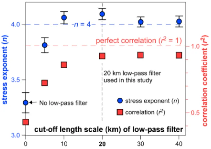
Data analysis was restricted to areas whereH>200 m. As the SIA is only an appropriate approximation of the stress state in the ice sheet away from the fast-flowing ice streams, the ice sheet margins and divides (Kirchner et al., 2016), we only take into account data from areas away from these (except for divides, which are discussed below). The driving stress (τ) was obtained from the surface gradient, using equation (3) (Figure 1b). Absolute surface velocities (v_s) and directions of surface flow were obtained from the MEaSUREs velocity data set (Joughin et al., 2010a, 2010b) with data from the years 2000–2008. The surface elevation of GrIS shows undulations and, hence, variations in surface slope, on the 5- to 20-km scale (Sergienko et al., 2014). Surface roughness was removed with a low-passfilter applied to the surface elevation data. After considering several cutoff wavelengths, we found that a 20-km low-passfilter gives the optimal compromise between spatial resolution and data quality, with a smooth distribution ofτ(Figures 1b and 2) and a good alignment of the directions of observed surface velocities v_s and τ, except near divides (Figure S1b in the supporting information). The alignment is a prerequisite for the validity of equation (2).

Furthermore, 20 km is about 10 times the ice sheet thickness, at which distance longitudinal stresses are eliminated, making the SIA an appropriate approach (Kamb & Echelmeyer, 1986).

4. Results and Discussion

From equation (2) it follows that

log v_s

H ¼nlogð Þ þτ CwithC¼ log 2A nþ1þv_base

Hτⁿ

(4)

Thus, a double logarithmic plot of the ratiov_s/Hand the driving stressτcan be used to determine the stress exponentnfrom a linear regression. This double logarithmic plot now shows a good correlation (Figure 3).

10.1029/2018GL078356

Geophysical Research Letters

Scatter in thev_s/Hdata can in part be explained by noise and errors in the velocity and bedrock elevation data. With a noise in the order of ±1 m/year in the velocity data, errors are in the order of ±15% at τ= 0.05 MPa, but lower at higher τ. The stress exponent (n) was determined fromv_s/H andτdata in a 328,162-km²reference area (Figure 1a). A value ofn= 4.10 was obtained from linear regression of the data points on the log (v_s/H) versus log (τ) graph (Figure 3), for points where τ > 0.04 MPa (87% of the reference area). The regression gives a standard error ofr² = 0.925 and 95% bootstrapped confidence limits at 4.04 and 4.14.

Assumingn= 4 and no basal motion, log (A’) was calculated for each data point with log (A’) = log (v_s/H)-4τ. Theflow factorA_{n= 4}forn= 4 was then obtained by averaging allA’values and usingA_{n= 4}=〈A⁰〉·(n+ 1)/2 (based on equation (2)). The rate factor thus obtained for the reference area is A_{n= 4}= 3.3 · 10⁵MPa⁴s¹. As with the publishedA_{n= 3}= 1.2 · 10⁶MPa³s¹for GrIS of Rignot and Mouginot (2012), this is an average rate factor for the whole ice sheet region under consideration.

Theflow factorAis a function of a number of state variables, such as lattice preferred orientation (Faria et al., 2014; Graham et al., 2018; Treverrow et al., 2012), grain size (de Bresser et al., 2001; Platt & Behr, 2011), Figure 1.Results of the analysis for the northern Greenland Ice Sheet. (a) Map of northern Greenland showing the surface velocity (v_s) distribution, the main ice streams and deep drilling sites, and the outline of the reference area. (b) Map of the driving stress (τin MPa) calculated with equation (3), using surface elevation data that were subjected to a 20-km low- passfilter. (c) Map of the surface velocity component(v_{ice,n= 4}), caused by internal shearing of the ice, calculated with the newn= 4flow law. (d) Predicted basal velocity, calculated by subtractingv_{ice,n= 4}fromv_s.

impurity content (Faria et al., 2009; Paterson, 1991), and temperature.

The data plotted in Figure 3 are sampled over a large reference area in which one or more of these variables may potentially vary systematically withτ. If this variation correlates withτ, the slope in thev_s/Hversusτplot would change and anapparent n-valuewould be obtained. It has been argued that glacial ice is softer than Holocene ice, due to the difference in impurity content (Faria et al., 2009; Paterson, 1991). The relative propor- tion of glacial ice decreases from the divides toward the margins (MacGregor et al., 2015). This would imply a negative correlation between Aandτand would actually lower the apparentn. Basal temperature is expected to increase, lattice preferred orientation to strengthen, and grain size to decrease with increasingτtoward the margins. Unfortunately, it is not known by how much, because very few direct measurements are available as most drill holes were sunk on divides or close to the ice sheet margin. It would be highly coincidental if the variation in these variables would correlate withτ to raise the slope in Figure 3 from the usually assumed n= 3 to exactly four over a large area in the ice sheet. We therefore assume that the observed slope in Figure 3 reflects the stress exponent to be used in theflow law (equation (1)).

It is of interest to note that Glen (1955) himself wrote“... it is noteworthy that practically observable long-time creep rates, as in a glacier, would probably depend on a higher power of the stress than the 3.2 found here.” One should note that Glen’s law is typically based on the stress/strain rate points from the minimum strain rate or peak/yield stress (Budd & Jacka, 1989; Glen, 1955), rather than those corresponding to steady state flow or tertiary creep. Glen (1955) derives a strain rate minimumnvalue of 3.2 and shows (Figure 12 in Glen, 1955) data for quasi-viscous creep rate that given = 4. More recent experiments (Qi et al., 2017;

Treverrow et al., 2012) give a peak stress (=minimum strain rate)nvalue of ~3, but a steady stateflow stress nvalue closer to 4, consistent with then= 4flow law derived by Durham et al. (1983) and Azuma and Higashi (1984). Considering the highfinite strains prevalent in ice sheets, the use of steady stateflow data appears to be more appropriate, as is corroborated by our in situ determination ofn= 4. Another factor may be that an apparentn= 3 could result from erroneouslyfitting a stress exponent to data that have been derived in the stress range at the transition between the dislocation creep regime (n= 4) and the regime of basal dislocation glide accompanying grain-boundary sliding (n = 1.8; Goldsby & Kohlstedt, 2001). The good correlation between the ratiov_s/Hand the driving stressτthat givesn= 4 breaks down at lowτ, which is mostly the case at divides. First, the SIA model does not apply at domes and divides, because flattening stresses cannot be ignored here (Kirchner et al., 2016; Raymond, 1983). This leads to fasterflow than predicted by the SIA model and deviating flow directions (Figure S1). Second, grain size-sensitive creep mechanisms may contribute significantly toflow at low stresses, reducing the stress exponent (Goldsby, 2006; Goldsby

& Kohlstedt, 2001; Pettit & Waddington, 2003). The transition to this low-stress regime has been proposed to range from 0.02 to 0.05 MPa (Budd & Jacka, 1989; Pettit & Waddington, 2003). Our data suggest that n= 4 applies to driving stresses above about 0.04 MPa (Figure 3), which is in agreement with the aforementioned studies.

The choice of the stress exponent is of utmost importance in determin- ing the amount of basal motion in Greenland’s ice sheet. A stress expo- nent that is too low leads to an overestimate of the viscosity at high driving stresses and, therefore, an underestimate of the internal defor- mation velocityv_ice. This in turn leads to an overestimate of the basal velocity, v_base. Using the same approach as Rignot and Mouginot (2012) and MacGregor et al. (2016), we mapped the ratio and difference of the actualv_sand the one predicted with the measuredn= 4flow law (v_{ice,n= 4}) for internal shearing of the ice only (Figures 1c and 1d). Basal Figure 2.Effect of the choice of low-passfilter on the linear regression of the

logarithms of the mean vertical shear strain rate (v_s/H)versusthe driving stress (τ) data. Blue circles: Stress exponent (n) with error bars representing the 95%

bootstrapped confidence intervals. Red squares: Correlation coefficient (r²).

Figure 3.Log (v_s/H)versuslog (τ) based on data in the reference area. The clas- sicaln= 3flow law (Rignot & Mouginot, 2012) and our new bestfitflow law with n= 4 are shown (see supporting information data set DS01 for the raw data).

10.1029/2018GL078356

Geophysical Research Letters

motion is most likely in areas where the ratiov_s/v_{ice,n= 4}exceeds two (then= 4 law accounts for<50% of the actual surface velocity) and where the actual surface velocity exceedsv_{ice,n= 4}by≥20 m/year (Rignot &

Mouginot, 2012; Figure 4). Both indicators for basal motion are fulfilled in ~6% of the northern GrIS area whereτ>0.04 MPa, while only one of the two criteria is fulfilled in another ~7%. Enhanced velocities are found at the margins of the ice sheet and at ice streams. The enhanced velocities (most distinct in Northeast Greenland Ice Stream (NEGIS)) are clear indications for an additional transport mechanism, most probably basal motion due to a thawed base (Fahnestock et al., 2001). However, the use of n = 4 significantly reduces the area with significant basal motion compared to current estimates that are based on ann= 3 rheology (MacGregor et al., 2016; Rignot & Mouginot, 2012).

When calculating the mismatch between observed velocities and calculated velocities withn= 4, our results indicate that the base of the ice may be thawed at the location of NorthGrip (Dahl-Jensen et al., 2003; but note thatτ<0.04; Figure 4). NorthGrip lies in the west of a large area that includes the onset of NEGIS and where large patches of basal melting are indicated, consistent with enhanced geothermal heatflow in this region (Fahnestock et al., 2001; Rogozhina et al., 2016).

5. Conclusions

A stress exponent of four has now been determined in situ, for thefirst time in a large area in an ice sheet, consistent with experimental data that use theflow or steady strain rate/stress (Durham et al., 1983; Qi et al., 2017; Treverrow et al., 2012) rather than the strain rate minimum or peak stress and in situ measure- ments on much smaller areas (Gillet-Chaulet et al., 2011). Above, we highlighted the implications of a higher nthan commonly assumed on estimates of the amount of basal motion in the northern part of GrIS. Since the Figure 4.Distribution of the likelihood of basal motion. We use two criteria: (i) the surface velocity (v_s) is more than double the predicted basal velocity (v_base) and (ii)v_sminusv_baseexceeds 20 m/year. Basal motion ismost likelywhen both criteria apply, andprobablewhen one of two applies. Areas deemedlikely thawedby MacGregor et al. (2016) and areas wherev_s exceeds the velocity predicted by then= 3flow law (v_{ice,n= 3}) by≥20 m/year according to Rignot and Mouginot (2012) are much larger than predicted by ourn= 4flow law. Areas where the driving stress is less than 0.04 MPa are shown with dashes.

stress exponent is a material property of ice, this observation is not restricted to GrIS but also applicable to the Antarctic Ice Sheet and mountain glaciers. However, the implications reach much further. (i) Strong, centimeter-scaleflow heterogeneity in ice is observed in numerical simulations of ice deformation (Llorens et al., 2016; usingn= 3) and disturbances in layering in ice cores (Jansen et al., 2016). Our unpublished simu- lations show that the heterogeneity increases whennis raised and extends to all scales, as is observed in rocks (Carreras, 2001; de Riese et al., 2018). (ii) Overestimating basal motion can lead to misinterpretations of the cause for large-scale folding observed in radar stratigraphy (compare Wolovick et al., 2014, and Bons et al., 2016). (iii) The vertical-velocity profile depends onn. As a consequence, the total massflux at a given surface velocity and ice thickness is about 5% higher forn= 4 compared ton= 3. Models that usen= 3 (Gillet-Chaulet et al., 2012; Graversen et al., 2011; Karlsson & Dahl-Jensen, 2015; Ren et al., 2011) may thus underestimate icefluxes or may compensate for this by invoking basal motion. Increasingnalso reduces the kink-point heighthin the velocity profile that is used in the Dansgaard-Johnsen model to predict age- depth relationships (Dansgaard & Johnsen, 1969). This has implications for inferences on the amount of basal melting based on measurements ofh(e.g., Fahnestock et al., 2001; MacGregor et al., 2016). (iv) The even stronger nonlinearity withn= 4 means that the ice sheet is responding faster to changes in boundary con- ditions, which also means that changing and retreating grounding lines can affect theflux of inland ice in shorter times (Gillet-Chaulet et al., 2011). It remains to be determined whether these implications in combi- nation make ice sheets less or more stable under changing conditions. What can be inferred is that the inter- nal deformation of ice plays a bigger role than hitherto assumed. Considering the importance of correctly predicting ice sheet behavior and related sea level rise, with results of models feeding into global political- economical decisions, it is imperative that iceflow modelers start consideringn= 4, at least as an alternative to onlyn= 3.

References

Azuma, N., & Higashi, A. (1984). Mechanical properties of Dye 3 Greenland deep ice cores.Annals of Glaciology,5, 1–8. https://doi.org/

10.3189/1984AoG5-1-1-8

Bamber, J. L., Griggs, J. A., Hurkmans, R. T. W. L., Dowdeswell, J. A., Gogineni, S. P., Howat, I., et al. (2013). A new bed elevation dataset for Greenland.The Cryosphere,7(2), 499–510. https://doi.org/10.5194/tc-7-499-2013

Bell, R. E., Tinto, K., Das, I., Wolovick, M., Chu, W., Creyts, T. T., et al. (2014). Deformation, warming and softening of Greenland’s ice by refreezing meltwater.Nature Geoscience,7, 497–502. https://doi.org/10.1038/ngeo2179

Bons, P. D., Jansen, D., Mundel, F., Bauer, C. C., Binder, T., Eisen, O., et al. (2016). Convergingflow and anisotropy cause large-scale folding in Greenland’s ice sheet.Nature Communications,7, 11427. https://doi.org/10.1038/ncomms11427

Budd, W. F., & Jacka, T. H. (1989). A review of ice rheology for ice sheet modeling.Cold Regions Science and Technology,16, 107–144.

Carreras, J. (2001). Zooming on Northern Cap de Creus shear zones.Journal of Structural Geology,23, 1457–1486. https://doi.org/10.1016/

S0191-8141(01)00011-6

Clark, P. U., Shakun, J. D., Marcott, S. A., Mix, A. C., Eby, M., Kulp, S., et al. (2016). Consequences of twenty-first-century policy for multi- millennial climate and sea-level change.Nature Climate Change,6(4), 360–369. https://doi.org/10.1038/nclimate2923

Cuffey, K. M., & Kavanaugh, J. L. (2011). How nonlinear is the creep deformation of polar ice? A newfield assessment.Geology,39, 1027–1030.

https://doi.org/10.1130/G32259.1

Dahl-Jensen, D., Gundestrup, N., Gogineni, S. P., & Miller, H. (2003). Basal melt at NorthGRIP modeled from borehole, ice-core and radio-echo sounder observations.Annals of Glaciology,37, 207–212. https://doi.org/10.3189/172756403781815492

Dansgaard, W., & Johnsen, S. J. (1969). Aflow model and a time scale for the ice core from Camp Century, Greenland.Journal of Glaciology, 8(53), 215–233.

de Bresser, J., ter Heege, J., & Spiers, C. (2001). Grain size reduction by dynamic recrystallization: Can it result in major rheological weakening?

International Journal of Earth Sciences,90, 28–45. https://doi.org/10.1007/s005310000149

de Riese, T., Bons, P. D., Gomez-Rivas, E., Griera, A., Llorens, M.-G., & Ran, H. (2018). Shear localisation in homogeneous, mechanically aniso- tropic materials.Geophysical Research Abstracts,20, EGU2018–EGU11875.

Durham, W. B., Heard, H. C., & Kirby, S. H. (1983). Experimental deformation of poly-crystalline H2O ice at high pressure and low temperature:

Preliminary results.Journal of Geophysical Research,88, B377–B392. https://doi.org/10.1029/JB088iS01p0B377

Fahnestock, M., Abdalati, W., Joughin, I., Brozena, J., & Gogineni, P. (2001). High geothermal heatflow, basal melt, and the origin of rapid ice flow in Central Greenland.Science,294, 2338–2342. https://doi.org/10.1126/science.1065370

Faria, S. H., Kipfstuhl, S., Azuma, N., Freitag, J., Hamann, I., Murshed, M. M., & Kuhs, W. F. (2009). The multiscale structure of Antarctica. Part I:

Inland ice.Low Temperature Science,68, 39–59.

Faria, S. H., Weikusat, I., & Azuma, N. (2014). The microstructure of polar ice. Part II: State of the art.Journal of Structural Geology,61, 21–49.

https://doi.org/10.1016/j.jsg.2013.11.003

Gillet-Chaulet, F., Gagliardini, O., Seddik, H., Nodet, M., Durand, G., Ritz, C., et al. (2012). Greenland ice sheet contribution to sea-level rise from a new-generation ice-sheet model.The Cryosphere,6(6), 1561–1576. https://doi.org/10.5194/tc-6-1561-2012

Gillet-Chaulet, F., Hindmarsh, R. C. A., Corr, H. F. J., King, E. C., & Jenkins, A. (2011). In-situ quantification of ice rheology and direct mea- surement of the Raymond Effect at Summit, Greenland using a phase-sensitive radar.Geophysical Research Letters,38, L24503. https://doi.

org/10.1029/2011GL049843

Glen, J. W. (1952). Experiments on the deformation of ice.Journal of Glaciology,2, 111–114.

Glen, J. W. (1955). The creep of polycrystalline ice.Proceedings of the Royal Society of London A: Mathematical, Physical and Engineering Sciences,228(1175), 519–538. The Royal Society.

10.1029/2018GL078356

Geophysical Research Letters

Acknowledgments

This research was funded by HGF-grant VH-NG-802 to D. J. and I. W. M. G. L. was funded by the programme for Recruitment of Excellent Researchers of the Eberhard Karls University Tübingen.

We thank Nobuhiko Azuma and Ed Waddington for their careful reviews.

Surface and bedrock elevation data were kindly provided by J. L. Bamber. An older, lower-resolution data set can be obtained from NSIDC (http://nsidc.org/

data/nsidc-0092). Surface velocities (Joughin et al., 2010a, 2010b) can be obtained from NSIDC (http://nsidc.org/

data/NSIDC-0670). Derived data are available from the PANGAEA repository at https://doi.pangaea.de/10.1594/

PANGAEA.890558 (doi: 10.1594/

PANGAEA.890558). These are maps of the surface elevation (S), ice thickness (H), driving stress, thevs/Hratio, predicted surface velocity forn= 4 (vice), and the predicted basal velocity for n = 4 (vbase). Data plotted in Figure are provided as supporting

information Data Set S1.

Goldsby, D. L. (2006). Superplasticflow of ice relevant to glacier and ice-sheet mechanics. In P. G. Knight (Ed.),Glacier Science and Environmental Change(pp. 308–314). Oxford: Blackwell.

Goldsby, D. L., & Kohlstedt, D. L. (2001). Superplastic deformation of ice: Experimental observations.Journal of Geophysical Research,106, 11,017–11,030. https://doi.org/10.1029/2000JB900336

Graham, F. S., Morlighem, M., Warner, R. C., & Treverrow, A. (2018). Implementing an empirical scalar constitutive relation for ice withflow- induced polycrystalline anisotropy in large-scale ice sheet models.The Cryosphere,12, 1047–1067. https://doi.org/10.5194/tc-12-1047- 2018

Graversen, R. G., Drijfhout, S., Hazeleger, W., van de Wal, R., Bintanja, R., & Helsen, M. (2011). Greenland’s contribution to global sea-level rise by the end of the 21st century.Climate Dynamics,37(7–8), 1427–1442. https://doi.org/10.1007/s00382-010-0918-8

Hewitt, I. J. (2013). Seasonal changes in ice sheet motion due to melt water lubrication.Earth and Planetary Science Letters,371–372, 16–25.

https://doi.org/10.1016/j.epsl. 2013.04.022

Hooke, R. (1981). Flow law for polycrystalline ice in glaciers: Comparison of theoretical predictions, laboratory data, andfield measurements.

Reviews of Geophysics and Space Physics,19, 664–672. https://doi.org/10.1029/RG019i004p00664

Hutter, K. (1983). Theoretical glaciology; material science of ice and the mechanics of glaciers and ice sheets.D. Reidel Publishing Co., Dordrecht, Terra Scientific Publishing Co, Tokyo.

Intergovernmental Panel on Climate Change (2014). Climate Change 2014: Synthesis Report. In Core Writing Team, R. K. Pachauri, &

L. A. Meyer (Eds.),Contribution of Working Groups I, II and III to the Fifth Assessment Report of the Intergovernmental Panel on Climate Change (p. 151). Geneva, Switzerland: IPCC.

Jansen, D., Llorens, M.-G, Westhoff, J., Steinbach, F., Kipfstuhl, S., Bons, P. D., et al. (2016). Small-scale disturbances in the stratigraphy of the NEEM ice core: Observations and numerical model simulations.The Cryosphere,10, 359–370. https://doi.org/10.5194/tc-10-359-2016 Joughin, I., Smith, B., Howat, I., & Scambos, T. (2010a).MEaSUREs Greenland Ice velocity map from InSAR data. Boulder, Colorado, USA: NASA

DAAC at the National Snow and Ice Data Center. https://doi.org/10.5067/MEASURES/CRYOSPHERE/nsidc-0478.001

Joughin, I., Smith, B., Howat, I. M., Scambos, T., & Moon, T. (2010b). Greenlandflow variability from ice-sheet-wide velocity mapping.Journal of Glaciology,56, 415–430. https://doi.org/10.3189/002214310792447734

Kamb, B., & Echelmeyer, K. A. (1986). Stress-gradient coupling in glacierflow 1. Longitudinal averaging of the influence of ice thickness and surface slope.Journal of Glaciology,32, 267–284. https://doi.org/10.3189/S0022143000015604

Karlsson, N. B., & Dahl-Jensen, D. (2015). Response of the large-scale subglacial drainage system of Northeast Greenland to surface elevation changes.The Cryosphere,9, 1465–1479. https://doi.org/10.5194/tc-9-1465-2015

Kirchner, N., Ahlkrona, J., Gowan, E. J., Lötstedt, P., Lea, J. M., Noormets, R., et al. (2016). Shallow ice approximation, second order shallow ice approximation, and full Stokes models: A discussion of their roles in palaeo-ice sheet modelling and development.Quaternary Science Reviews,147, 136–147. https://doi.org/10.1016/j.quascirev.2016.01.032

Llorens, M. G., Griera, A., Bons, P. D., Lebensohn, R. A., Evans, L. A., Jansen, D., & Weikusat, I. (2016). Full-field predictions of ice dynamic recrystallisation under simple shear conditions.Earth and Planetary Science Letters,450, 233–242. https://doi.org/10.1016/j.

epsl.2016.06.045

MacGregor, J. A., Fahnestock, M. A., Catania, G. A., Aschwanden, A., Clow, G. D., Colgan, W. T., et al. (2016). A synthesis of the basal thermal state of the Greenland Ice Sheet.Journal of Geophysical Research: Earth Surface,121, 1328–1350. https://doi.org/10.1002/2015JF003803 MacGregor, J. A., Fahnestock, M. A., Catania, G. A., Paden, J. D., Gogineni, S. P., Young, S. K., et al. (2015). Radiostratigraphy and age structure of

the Greenland Ice Sheet.Journal of Geophysical Research: Earth Surfarce,120, 212–241. https://doi.org/10.1002/2014JF003215 Paterson, W. S. B. (1991). Why ice-age ice is sometimes“soft”.Cold Regions Science and Technology,20, 75–98. https://doi.org/10.1016/0165-

232X(91)90058-O

Pettit, E. C., & Waddington, E. D. (2003). Iceflow at low deviatoric stress.Journal of Glaciology,49, 359–369. https://doi.org/10.3189/

172756503781830584

Platt, J. P., & Behr, W. M. (2011). Grain size evolution in ductile shear zones: Implications for strain localization and the strength of the lithosphere.Journal of Structural Geology,33, 537–550. https://doi.org/10.1016/j.jsg.2011.01.018

Qi, C., Goldsby, D. L., & Prior, J. P. (2017). The down-stress transition from cluster to cone fabrics in experimentally deformed ice.Earth and Planetary Science Letters,471, 136–147. https://doi.org/10.1016/j.epsl.2017.05.008

Raymond, C. F. (1983). Deformation in the vicinity of ice divides.Journal of Glaciology,29, 357–373. https://doi.org/10.3189/

S0022143000030288

Ren, D., Fu, R., Leslie, L. M., Chen, J., Wilson, C., & Karoly, D. J. (2011). The Greenland Ice Sheet response to transient climate change.Journal of Climate,24, 3469–3483. https://doi.org/10.1175/2011JCLI3708.1

Rignot, E., & Mouginot, J. (2012). Iceflow in Greenland for the International Polar Year 2008–2009.Geophysical Research Letters,39, L11501.

https://doi.org/10.1029/2012GL051634

Rogozhina, I., Petrunin, A. G., Vaughan, A. P., Steinberger, B., Johnson, J. V., Kaban, M. K., et al. (2016). Melting at the base of the Greenland ice sheet explained by Iceland hotspot history.Nature Geoscience,9(5), 366–369. https://doi.org/10.1038/ngeo2689

Sergienko, O. V., Creyts, T. T., & Hindmarsh, R. C. A. (2014). Similarity of organized patterns in driving and basal stresses of Antarctic and Greenland ice sheets beneath extensive areas of basal sliding.Geophysical Research Letters,41, 3925–3932. https://doi.org/10.1002/

2014GL059976

Stokes, C. R., Clark, C. D., Lian, O. B., & Tulaczyk, S. (2007). Ice stream sticky spots: A review of their identification and influence beneath contemporary and palaeo-ice streams.Earth-Science Reviews,81, 217–249. https://doi.org/10.1016/j.earscirev.2007.01.002

Treverrow, A., Budd, W., Jacka, T., & Warner, R. (2012). The tertiary creep of polycrystalline ice: Experimental evidence for stress dependent levels of strain-rate enhancement.Journal of Glaciology,58, 301–314. https://doi.org/10.3189/2012JoG11J149

Weertman, J. (1983). Creep deformation of ice.Annual Review of Earth and Planetary Sciences,11(1), 215–240.

Wolovick, M. J., Creyts, T. T., Buck, W. R., & Bell, R. E. (2014). Traveling slippery patches produce thickness-scale folds in ice sheets.Geophysical Research Letters,41, 8895–8901. https://doi.org/10.1002/2014GL062248