Chapter 13: Reactions at the Earth’s Surface:

Chapter 13: Reactions at the Earth’s Surface:

Weathering, Soils, and Stream Chemistry

Introduction

he geochemistry of the Earth's surface is dominated by aqueous solutions and their interactions with rock. We saw in the last chapter that the upper continental crust has the approximate average composition of granodiorite, and that the oceanic crust consists of basalt. But a random sample of rock from the crust is unlikely to be either; indeed it many not be an igneous rock at all. At the very surface of the Earth, sediments and soils predominate. Both are ultimately produced by t h e interaction of water with Òcrystalline rockÓ (by which we mean igneous and metamorphic rocks).

Clearly, to fully understand the evolution of the Earth, we need to understand the role of geochemi- cal processes involving water.

Beyond that, water is essential to life and central to human activity. We use water for drinking, cooking, agriculture, heating, cooling, resource recovery, industrial processing, waste disposal, trans- portation, fisheries, etc. Water chemistry, i.e., the nature of solutes dissolved in it, is the primary factor in the suitability of water for human use. ÒPollutedÓ water is unsuitable for drinking and cook- ing; saline water is unsuitable for these uses as well as agriculture and many industrial uses, etc. W e have been particularly concerned with water pollution in the past few decades; that is with the im- pact of human activity on water chemistry. Both our advancing technology and our exponentially in- creasing numbers have made pollution problems progressively worse, particularly over the past cen- tury. However, we have also become more aware of the adverse impact of poor water quality on hu- man health and the quality of life, and perhaps less tolerant of it as well.

Understanding and addressing problems of water pollution requires an understanding of the behav- ior of natural aqueous systems for at least two reasons. First, to identify pollution, we need to know the characteristics of natural systems. For example, Pb can be highly toxic, and high concentrations of Pb in the blood have been associated with learning disabilities and other serious problems. How- ever, essentially all waters have some finite concentration of Pb; we should be concerned only when Pb concentrations exceed natural levels. Second, natural processes affect pollutants in the same way they affect their natural counterparts. For example, cadmium leached from landfills will be subject to the same adsorption/desorption reactions as natural Cd. To predict the fate of pollutants, we need to understand those processes.

In this chapter, we focus on water and its interaction with solids at the EarthÕs surface. We can broadly distinguish two kinds of aqueous solutions: continental waters and seawater. Continental wa- ters by this definition include ground water, fresh surface waters (river, stream and lake waters), and saline lake waters. The compositions of these fluids are obviously quite diverse. Seawater, on t h e other hand, is reasonably uniform, and it is by far the dominant fluid on the earth's surface. Hy- drothermal fluids are third class of water produced when water is heated and undergoes accelerated interactions with rock and often carry a much higher concentration of dissolved constituents than fresh water. Our focus in this chapter will be on the chemistry of continental waters and how they interact with rock. We we consider seawater in Chapter 15.

Redox in Natural Waters

The surface of the Earth represents a boundary between regions of very different redox state. The atmosphere contains free oxygen and therefore is highly oxidizing. In the EarthÕs interior, however, there is no free oxygen, Fe is almost entirely in the 2+ valance state, reduced species such as CH4, CO, and S2 exist, and conditions are quite reducing. Natural waters exist in this boundary region and their redox state, perhaps not surprisingly, is highly variable. Biological activity is the principal cause of this variability. Plants (autotrophs) use solar energy to drive thermodynamically unfavorable

T

photosynthetic reactions that produce free O2, the ultimate oxidant, on the one hand and organic matter, the ultimate reductant, on the other. Indeed it is photosynthesis that is responsible for t h e oxidizing nature of the atmosphere and the redox imbalance between the EarthÕs exterior and inte- rior. Both plants and animals (heterotrophs) liberate stored chemical energy by catalyzing the oxi- dation of organic matter in a process called respiration. The redox state of solutions and solids at t h e EarthÕs surface is largely governed by the balance between photosynthesis and respiration. By this we mean that most waters are in a fairly oxidized state because of photosynthesis and exchange with the atmosphere. When they become reducing, it is most often because respiration exceeds photosyn- thesis and they have been isolated from the atmosphere. Water may also become reducing as a result of reaction with sediments deposited in ancient reduced environments, but the reducing nature of those ancient environments resulted from biological activity. Weathering of reduced primary igneous rocks also consumes oxygen, and this process governs the redox state of some systems, mid-ocean ridge h y - drothermal solutions for example. On a global scale, however, these processes are of secondary im- portance for the redox state of natural waters.

The predominant participants in redox cycles are C, O, N, S, Fe, and Mn. There are a number of other elements, for example, Cr, V, As, and Ce, that have variable redox states; these elements, however, are always present in trace quantities and their valance states reflect, rather than control, the redox state of the system. Although phosphorus has only one valance state (+V) under natural conditions, its concentration in solution is closely linked to redox state because the biological reactions that control redox state also control phosphorus concentration, and because it is so readily adsorbed on Fe oxide surfaces.

Water in equilibrium with atmospheric oxygen has a pε of +13.6 (at pH = 7). At this pε, thermody- namics tells us that all carbon should be present as CO2 (or related carbonate species), all nitrogen as NO ^3±, all S as SO ^42±, all Fe as Fe³⁺, and all Mn as Mn⁴⁺. This is clearly not the case and this dise- quilibrium reflects the kinetic sluggishness of many, though not all, redox reactions^£. Given the dise- quilibrium we observe, t h e

applicability of thermody- namics to redox systems would appear to be limited.

Thermodynamics may never- theless be used to develop partial equilibrium models.

In such models, we can make use of redox couples t h a t might reasonably be at equi- librium to describe the redox state of the system. In Chap- ter 3, we introduced the tools needed to deal with redox reactions: EH, the hydrogen scale potential (the poten- tial developed in a standard hydrogen electrode cell) and pε, or electron activity. W e found that both may in turn be related to the Gibbs Free Energy of reaction through

£ While this may make life difficult for geochemists, it is also what makes it possible in the first place. We, like all other organisms, consist of a collection of reduced organic species that manage to persist in an oxidizing environment!

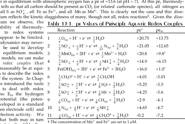
Table 13.1. pe Values of Principle Aquatic Redox Couples

Reaction pε¡ pεW

1 1

4O2(g) + H⁺ + e^Ð ®

1

2H2O +20.75 +13.75

2

1

5NO ₃^± +

6

5H⁺ + e^Ð ®

1 10N2(g) +

3

5H2O +21.05 +12.65 3

1

2MnO2(s) + 2H⁺ + e^Ð ®

1

2Mn²⁺ + H2O +20.8 +9.8 4

5

4NO ₃^± +

6

5H⁺ + e^Ð ®

1

8NH4+ +

3

8H2O +14.9 +6.15 5 Fe(OH)3(s) + 3H⁺ + e^Ð ® Fe²⁺ + 3H2O +16.0 +1.0 6

1

2CH2O* + H⁺ + e^Ð ®

1

2CH3OH +4.01 -3.01

7 1 8SO ₄^2- +

5

4H⁺ + e^Ð ®

1 8H2S +

1

2H2O +5.25 -3.5 8

1 8SO ₄^2- +

9

8H⁺ + e^Ð ®

1 8HS^Ð +

1

2H2O +4.25 -3.6 9

1

8CO2(g) + H⁺ + e^Ð ®

1

8CH4(g) +

1

4H2O +2.9 -4.1

10 ¹₆N2(g) +

4

3H⁺ + e^Ð ®

1

3NH₄⁺ +4.65 -4.7

11 1

4CO2(g) + H⁺ + e^Ð ®

1

4CH2O* +

1

4H2O -0.2 -7.2 The concentration of Mn²⁺ and Fe²⁺ are set to 1 µM.

* We are using ÒCH₂OÓ, which is formally formaldahyde, as an abbreviation for organic matter generally (for example, glucose is C₆H₁₂O₆).

the Nernst Equation (equ. 3.121). These are all the tools we need; in this section, we will see how we can apply them to understanding redox in aqueous systems.

Table 13.1 lists the pε¡ of the most important redox half reactions in aqueous systems. Also listed are pεW values. pεW is the pε¡ when the concentration of H⁺ is set to 10^-7 (pH = 7). The relation be- tween pε¡ and pεW is simply:

pεW = pε° + log [H⁺]^ν = pε° – ν × 7

Reactions are ordered by decreasing pεW from strong oxidants at the top to strong reductants at the bot- tom. In this order, each reactant can oxidize any product below it in the list, but not above it. Thus sulfate can oxidize methane to CO2, but not ferrous iron to ferric iron. Redox reactions in aqueous sys- tems are often biologically mediated. In the following section, we briefly explore the role of the bi- ota in controlling the redox state of aqueous systems.

Biogeochemical Redox Reactions

As we noted above, photosynthesis and atmospheric exchange maintains a high pε in surface wa- ters. Water does not transmit light well, so there is an exponential decrease in light intensity with depth. As a result, photosynthesis is not possible below depths of 200 m even in the clearest waters.

In murky waters, photosynthesis can be restricted to the upper few meters or less. Below this Òphotic zoneÓ, biologic activity and respiration continue, sustained by falling organic matter from the photic zone. In the deep waters of lakes and seas where the rate of respiration exceeds downward advection of oxygenated surface water, respiration will consume all available oxygen. Once oxygen is consumed, a variety of specialized bacteria continue to consume organic matter and respire utilizing oxidants other than oxygen. Thus pε will continue to decrease.

Since bateria exploit first the most energetically favorable reactions, Table 13.1 provides a guide the sequence in which oxidants are consumed as pε decreases. From it, we can infer that once all mo- lecular oxygen is consumed, reduction of nitrate to molecular nitrogen will occur (reaction 2). This processes, known as denitrification, is carried out

by bacteria, which use the oxygen liberated to oxidize organic matter and the net energy liber- ated to sustain themselves. At lower levels of pε, other bacteria reduce nitrate to ammonia (reaction 4), a process called nitrate reduction, again using the oxygen liberated to oxidize or- ganic matter. At about this pε level, Mn⁴⁺ will be reduced to Mn²⁺. At lower pε, ferric iron is reduced to ferrous iron. The reduction of both Mn and Fe may also be biologically mediated in whole or in part.

From Table 13.1, we can expect that fermenta- tion (reaction 6 in Table 13.1) will follow reduc- tion of Fe. Fermentation can involve any of a number of reactions, only one of which, reduction of organic matter (carbohydrate) to methanol, is represented in Table 13.1. In fermentation reac- tions, further reduction of some of the organic car- bon provides a sink of electrons, allowing oxida- tion of the remaining organic carbon; for example in glucose, which has 6 carbons, some are oxidized to CO2 while others are reduced to alcohol or ace- tic acid. While these kinds of reactions can be carried out by many organisms, it is bacterial-me-

4 5 6 7 8 9

pH -8

-4 0 4 8 12 18

pe

Fe(OH)

3

H₂S MnMnO_{2+ 2}

Fe₂₊

N₂

N₂

NO3–

SO₄^2–

NH4+

Fermentation

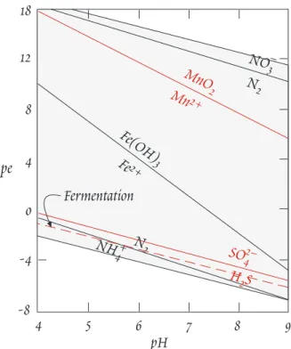
Figure 13.1. Important biogeochemical redox couples in natural waters.

diated fermenation that is of geochemical interest.

At lower pε, sulfate is used as the oxidant by sulfate-reducing bacteria to oxidize organic matter, and at even lower pε, nitrogen is reduced to ammonia (reaction 9), a process known as nitrogen f i x a - tion, with the nitrogen serving an the electron acceptor for the oxidization of organic matter. This re- action is of great biological importance, as nitrogen is an essential ingredient of key biological com- pounds such as proteins and DNA (see Chapter 14), and hence is essential to life; all plants must therefore take up inorganic nitrogen. While a few plants, blue-green algae (cyanobacteria) and leg- umes, can utilize N2, most require ÒfixedÓ nitrogen (ammonium, nitrate, or nitrite). Hence nitrogen- fixing bacteria play an essential role in sustaining life on the planet.

To summarize, in a water, soil, or sediment column where downward flux of oxygen is less than t h e downward flux of organic matter, we would expect to see oxygen consumed first, followed by reduction of nitrate, manganese, iron, sulfur, and finally nitrogen. This sequence is illustrated on a pε-pH dia- gram in Figure 13.1. We would expect to see a similar sequence with depth in a column of sediment where the supply of organic matter exceeds the supply of oxygen and other oxidants.

Eutrophication

The extent to which the redox sequence described above proceeds in a body of water depends on a several factors. The first of these is temperature structure, because this governs the advection of oxy- gen to deep waters. As mentioned above, light (and other forms of electromagnetic energy) is not transmitted well by water. Thus only surface waters are heated by the Sun. As the temperature of surface water rises, its density decreases (fresh water reaches it greatest density at 4¡ C). These warmer surface waters, known in lakes as the epilimnion, generally overlie a zone where temperature decreases rapidly, known as the thermocline or metalimnion, and a deeper zone of cooler water, known as the hypolimnion. This temperature stratification produces a stable density stratification which prohibits vertical advection of water and dissolved constitutents, including oxygen and nutri- ents. In tropical lakes and seas, this stratification is permanent. In temperate regions, however, there is an annual cycle in which stratification develops in the spring and summer. As the surface water cools in the fall and winter, its density decreases below that of the deep water and vertical mixing occurs. The second important factor governing the extent to which reduction in deep water oc- curs is nutrient levels. Nutrient levels limit the amount of production of organic carbon by photosyn- thesizers (in lakes, phosphorus concentrations are usually limiting; in the oceans, nitrate and micro- nutrients such as iron appear to be limiting). The availability of organic carbon in turn controls bio- logical oxygen demand (BOD) In water with high nutrient levels there is a high flux of organic car- bon to deep waters and hence higher BOD.

In lakes with high nutrient levels, the temperature stratification described above can lead to a situation where dissolved oxygen is present in the epilimnion and absent in the hypolimnion. Regions where dissolved oxygen is present are termed oxic, those where sulfide or methane are present are called anoxic. Regions of intermediate pε are called suboxic. Lakes are where suboxic or anoxic condi- tions exist as a result of high biological producitivy are said to be eutrophic. This occurs naturally in many bodies of water, particularly in the tropics where stratification is permanent. It can also occur, however, as a direct result addition of pollutants such as sewage to the water, and an indirect result of pollutants such as phosphate and nitrate. Addition of the latter enhances productivity and availability of organic carbon, and ultimately BOD. When all oxygen is consumed conditions become anaerobic and the body of water becomes eutrophic. Where this occurs naturally, ecosystems have adapted to this circumstance and only anaerobic bacteria are found in the hyperlimnion. When it re- sults from pollution, it can be catastrophic for macrofauna such as fish that cannot tolerate anaerobic conditions.

Redox and Biological Primary Production

The biota is capable of oxidations as well as reductions. The most familiar of these reactions is photosynthesis. Most organisms capable of photosynthesis, which includes both higher plants and a variety of single-celled organisms, produce oxygen as a biproduct of photosynthesis:

CO₂ + H₂O ® CH₂O + O₂ 13.1

However, there are also photosynthesis pathways that do not produce O2. Green and purple sulfur bacteria are phototrophs that oxidize sulfide to sulfur in the course of photosynthesis:

CO₂ + 2H₂S ® CH₂O +

1

4S₈ + H₂O 13.2

This reaction requires considerably less light energy (77.6 vs. 476 kJ/mol) than oxygenic photosynthe- sis, enabling these bacteria survive at lower light levels than green plants.

While photosynthesisis is far and away the primary way in which organic carbon is produced or ÒfixedÓ, chemical energy rather than light energy may also be used to fix organic carbon in processes collectively known as chemosynthesis. In chemosynthesis, the energy liberated in oxidizing reduced inorganic species is used to reduce CO2 to organic carbon. For example, nitrifying bacteria oxidize ammonium to nitrite in a process known as nitrification:

CO₂ +

2

3NH₄ +

1

3H₂O ® CH₂O +

2

3NO₂^– +

4

3H⁺ 13.3

Colorless sulfur bacteria oxidize sulfide to sulfate in fixing organic carbon:

CO₂ + H₂S + O₂ + H₂O ® CH₂O + SO₄²⁻ + 2H⁺ 13.4

Redox Buffers and Transition Metal Chemistry

The behavior of transition metals in aqueous solutions and solids in equilibrium with them is par- ticularly dependent on redox state. Many transition metals have more than one valence state within the range of pε of water. In a number of cases, the metal is much more soluble in one valence state than in others. The best examples of this behavior are provided by iron and manganese, both of which are much more soluble in their reduced (Fe²⁺, Mn²⁺) than in oxidized (Fe³⁺, Mn⁴⁺) forms. Redox conditions thus influence a strong control on the concentrations of these elements in natural waters.

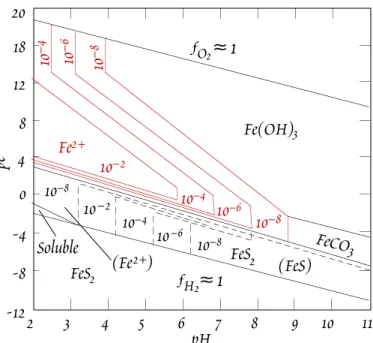
Because of the low solubility of their oxidized formes, the concentrations of Fe, Mn, and similar metals are quite low under ÒnormalÓ conditions, i.e., high pε and near- neutral pH. There two common circum- stances where higher Fe and Mn concentra- tions in water occur. The first is when sul- fide ores are exposed by mining and oxi- dized to sulfate, e.g.:

2FeS_2(s) + 2H₂O + 7O₂ ® 4H⁺ + 4SO₄²⁻ + 2Fe²⁺

This can dramatically lower the pH of streams draining such areas. The lower pH in turn allows higher concentrations of dis- solved metals (e.g., Figure 13.2), even under oxidizing conditions. The second circum- stance where higher Fe and Mn concentra- tions occur is under suboxic or anoxic condi- tions that may occur in deep waters of lakes and seas as well as sediment pore waters.

Under these circumstances Fe and Mn are

2 3 4 5 6 7 8 9 10 11

pH -12

-8 -4 0 4 8 12 18 20

Fe(OH)₃

FeS₂ (Fe²⁺)

ƒ_O2

Soluble

(FeS) 10^–6

10^–6 10^–8 10^–8

10^–4 10^–4

10^–2 10^–2

≈ 1

ƒ_H2≈ 1

FeCO3

pe 10–6 10–810–4

10^–8

FeS₂ Fe²⁺

Figure 13.2. Contours of dissolved Fe activity as a function of pε and pH.

reduced to their soluble forms, allowing much higher concentrations.

In cases where precipitation or solution involves a change in valence or oxidation state, the solubil- ity product must include pε or some other redox couple, e.g.:

Fe₂O₃ +6H⁺+2e^– ® 2Fe²⁺ +3H₂O K = a²_Fe²⁺

a_H⁶⁺a²_e^–

13.5

In Chapter 3, we noted that pε is often difficult to determine. One approach to the problem is to as- sume the redox state in the solution is controlled by a specific reaction. The controlling redox reac- tions will be those involving the most abundant species; very often this is sulfate reduction:

1

8SO₄²⁻ +

5

4H⁺ + e^- ®

1 8H₂S +

1

2H₂O 13.6

in which case pε is given by:

p p H S

SO pH

ε= ° −ε 1 − 8

4 5

2 4

ln [ 2]

[ ^–] 13.7

Under the assumption that this reaction controls the redox state of the solution, electrons may be eliminated from other redox reactions by substituting the above expression. For example, iron redox equilibrium may be written as:

1

8SO₄²⁻+

5

4H⁺ + Fe²⁺ ®

1 8H₂S +

1

2H₂O + Fe³⁺ 13.8

In this sense, the pε of most natural waters will be controlled by a redox buffer, a concept we consid- ered in Chapter 3. Example 13.1 illustrates this approach.

Example 13.1. Redox State of Lake Water

Consider water of the hypolimnion of a lake in which all oxygen has been consumed and with t h e following initial composition: SO4 = 2 × 10^-4 M, ΣFe³⁺ = 10^-6 M, Alk = 4 × 10^-4 eq/L, ΣCO2 = 1.0 × 10^-3 M, ΣÓCH2OÓ = 2 × 10^-4 M, pH = 6.3. Determine the pH, pε, and speciation of sulfur and iron when all or- ganic matter is consumed and redox equilibrium is achieved. The first dissociation constant of H2S is 10^Ð7.

Answer: LetÕs first consider the redox reactions involved. The species involved in redox reactions will be those of carbon, sulfur, and iron. The concentration of iron is small, so its oxidation state will reflect, rather than control, that of the solution. Thus oxidation of organic matter will occur though reduction of sulfate. We can express this by combining reactions 7 and 11 in Table 13.1 (we see from the dissociation constant that H2S will be the dominant sulfate species at pH below 7, so we chose reac- tion 7 rather than reaction 8):

1

2SO₄²⁻+ H⁺ + CH₂O ®

1

2H₂S +H₂O + CO₂ K=10^10.54 13.9

From the magnitude of the equilibrium constant (obtained from the pε¡Õs in Table 13.1), we can see that right side of this reaction is strongly favored. Since sulfate is present in excess of organic matter, this means sulfate will be reduced until all organic matter is consumed, which will leave equilmolar concentrations of sulfate and sulfide (10^-4 M each). Thus the redox state of the system will be gov- erned by that of sulfur. The redox state of iron can then be related to that of sulfur using reaction 13.8, for which we calculate an equilibrium constant of 10^-10.75 from Table 13.1.

The next problem we face is that of chosing components. As usual, we chose H⁺ as one component (and implicitly H2O as another). We will also want to chose a sulfur, carbon, and iron species as a component, but which ones? We could chose the electron as a component, but consistent with our conclu- sion above that the redox state of the system is governed by that of sulfur, a better choice is to chose both sulfate and sulfide, specifically H2S, as components. We can also see from Table 13.1 that Fe should be largely reduced, so we chose Fe²⁺ as the iron species. pH will be largely controlled by car- bonate species, since these are more than an order of magnitude more abundant than sulfate species;

oxidation of organic matter will increase the concentration of CO2, which will lower pH slightly. In

Figure 6.1, we can see that at pH below 6.4, H2CO3 will be the dominant carbonate species, so we chose this as the carbonate species. Our components are therefore H⁺, SO4, H2CO3, Fe²⁺, and H2S. The spe- cies of interest will include H⁺, OH^Ð, SO₄^{2 –}, H2S, HS^Ð, H2CO3, HCO₃⁻, as well as the various species of Fe (Fe²⁺, Fe³⁺, Fe(OH)²⁺, Fe(OH)₂⁺, Fe(OH)3 (we assume that the concentrations of CO₃²⁻, HSO₄^– and S^2- are neglible at this pH; we shall neglect them throughout).

Our next step is to determine pH. For TOTH we have:

TOTH = [H ⁺] – [OH^–] – [HCO₃^–] – [HS^–] + 5

4ΣFe³⁺ 13.10

The presence of the Fe³⁺ term may at first be confusing. To understand why it occurs, we can use equa- tion 13.7 to express Fe³⁺ as the algebraic sum of our components:

Fe³⁺= 1

8SO₄^2–+ 5

4H⁺+ Fe²⁺– 1

8 H₂S + 1

2H₂O 13.11

The first 4 terms on the right hand side of equation 13.10 are simply alkalinity plus additional CO2

produced by oxidation of organic matter, so 13.10 may be rewritten as:

TOTH = 5

4ΣFe³⁺– Alk – [CH₂O] 13.12

Inspecting equation 13.10, we see that HCO₃⁻is by far the largest term. Furthermore, the Fe term in equation 13.12 is neglible, so we have:

TOTH ∼– [HCO₃^–]∼6×10^–4 13.13

The conservation equation for carbonate is:

ΣH ₂CO₃= [H₂CO₃] + [HCO₃^–] =ΣCO₂+Σ[CH₂O] = 1.3×10^–3

Hence: H₂CO₃ = ΣΗ₂CO₃ – HCO₃⁻ = (1.3 – 0.6) × 10^-3

We can use this to calculate pH since: K = [HCO₃^–][H⁺]

[H₂CO₃] = 10^–6.35

Solving for [H⁺] and substitutiong values, we find that pH = 6.28.

For the conservation equation for sulfate, we will have to include terms for both Fe³⁺ (equation 13.11) and organic matter. Writing organic matter as the algebraic sum of our components we have:

CH₂O = 1

2 H₂S + H₂O + CO₂– 1

2SO₄^2–– H⁺

The amount of sulfate present will be that originally present less that used to oxidize organic matter.

The only other oxidant present in the system is ferric iron, so the amount of sulfide used to oxidize or- ganic matter will be the total organic matter less the amount of ferric iron initially present. The sul- fate conservation equation is then:

ΣSO ₄= [SO₄^2–] – 1

2ΣCH₂O + 1

8ΣFe³⁺∼1.0×10^–4M

(the Fe term is again neglible). The amount of sulfide present will be the amount created by oxidation of organic matter, less the amount of organic matter oxidized by iron, so the sulfide conservation equa- tion is:

ΣH₂S = H₂S + HS^–= + 1

2ΣCH₂O – 1

8ΣFe³⁺= 1×10^–4M 13.14

We now want to calculate the speciation of sulfide. We have

ΣH ₂S = H₂S + HS^–=1×10^–4M and K_1H

2S= [H⁺][HS^–]

[H₂S] = 10^–7

Solving these two equations, we have:

[HS ^–] = 10^–4

10⁷10^–6.23 = 1.92×10^–5

The concentration of H2S is then easily calculated as 8.08 × 10^-5 M. We can now calculate the pε of t h e solution by substituting the above values and the pε¡ in Table 13.1 for reaction 7 into equation 13.7.

Doing so, we find pε is -2.72. Finally, for iron we have:

ΣFe = [Fe ²⁺] +Σ[Fe³⁺] = 10^–6 and log [Fe²⁺]

[Fe³⁺] = pε– pε°= –2.72 – 13.0 = 15.78 13.15

so that Fe²⁺ = 10^15.78Fe³⁺. The equilibrium concentrations of the hydrolysis species of Fe³⁺ can be calcu- lated from equations 6.73a through 6.73d. We find the most abundant species will be Fe(OH)₂⁺, which is 10^6.8 times more abundant than Fe³⁺. However, Fe²⁺ remains 10^15.78 × 10^-6.9 more abundant t h a t Fe(OH)₂⁺, so for all practical purposes, all iron is present as Fe²⁺.

The development of anoxic conditions leads to an interesting cycling of iron and manganese within the water column. Below the oxic-anoxic boundary, Mn and Fe in particulates are reduced and dis- solved. The metals then diffuse upward to the oxic-anoxic boundary where they again are oxidized and precipitate. The particulates then migrate downward, are reduced, and the cycle begins again.

A related phenomena can occur within sediments. Even where anoxic conditions are not achieved within the water column, they can be achieved within the underlying sediment. Indeed, this will oc- cur where burial rate of organic matter is high enough to exceed the supply of oxygen. Figure 13.3 shows an example, namely a sediment core from southern Lake Michigan studied by Robbins and Cal- lender (1975). The sediment contains about 2% organic carbon in the upper few centimeters, which de- creases by a factor of 3 down core. The concentration of acid-extractable Mn in the solid phase (Figure 13.3a), presumably surface-bound Mn and Mn oxides, is constant at about 540 ppm in the upper 6 cm, but decreases rapidly to about 400 ppm by 12 cm. The concentration of dissolved Mn in the pore water in- creases from about 0.5 ppm to a maximum of 1.35 ppm at 5 cm and then subsuquently decreases (Figure 13.3) to a constant value of about 0.6 ppm in the bottom half of the core.

Because the Lake Michigan re- gion is heavily populated, it is tempting to interpret the data in Figure 13.3, particularly the in- crease in acid-extractable Mn near the core top, as being a result of recent pollution. However, Robbins and Callender (1975) demonstrated that the data could be explained with a simple steady-state diagentic model in- volving Mn reduction, diffusion, and reprecipitation (as MnCO3).

In Chapter 5, we derived the Di- agenetic Equation:

∂ c

∂t _x= ∂F

∂x _t+

Σ

The first term on the right is t h e change in total vertical flux with depth, the second is the sum of rates of all reactions occuring.

There are two potential flux

dC/dt (µg/cm³/yr) 0 3 6 9

Dissolution Rate 0 0.5 1.0 1.5Mn (ppm)

Pore Water

J J J J J

J J J J

J J

J J JJ JJ

400 450 500 550Mn (ppm) 0

5 10

15 20 25 30 35 40

Depth (cm) Solid phase

JJ JJ J J J

J J

J J J J J J

J

J

J a b c

Figure 13.3. (a) Concentration of acid-leachable Mn in Lake Michigan sediment as a function of depth. (b) (b) Dissolved Mn in pore water from the same sediment core. Solid line shows t h e dissolution-diffusion-reprecipitation model of Robbins and Calender (1975) constrained to pass through 0 concentration at 0 depth. Dashed line shows the model when this constraint is removed. (c) Dissolution rate of solid Mn calculated from rate of change of concentration of acid-leachable Mn and used to produce the model in (b). From Robbins and Calender (1975).

terms in this case, pore water advection (due ot compaction) and diffusion. There are also several re- action occurring: dissolution or desorption associated with reduction and a precipitation reaction. I f the system is at steady state, then ¶c/¶x = 0. Assuming steady-state, Robbins and Callender (1975) derived the following verision of the diagenetic equation:

φD d ²c

dx²– v dc

dx –φk₁(c – c_f) +φk₀(z) = 0 13.16

where φ is porosity (assumed to be 0.8), D is the diffusion coefficient, v is the advective velocity (-0.2 cm/yr), and k1 is the rate constant for reprecipitation reactions, and k0 is the dissolution rate (expressed as a function of depth). The first term is the diffusive term, the second the advective, t h e third the rate of reprecipitation, and the fourth is the dissolution rate. The dissolution rate must be related to the change in concentration of acid-extractable Mn. Thus the last term may be written as:

φk ₀(z) =φR φ∂c_s

∂x

where R is the sedimentation rate (g/cm²/yr) and cs is the concentration in the solid. Using least squares, Robbins and Callender found that the parameters that best fit the data were D = 9 × 10^-7 cm²/sec (30 cm²/yr) k1 = 1 yr^-1 and cf = 0.5 ppm. The solid line in Figure 12.44b represents the prediction of equation 13.16 using this values and assuming c0 (porewater concentration at the surface) is 0. The dashed line in Figure 13.3b assumes c0 = 0.6 ppm. The latter is too high, as c0 should be the same con- centration as lake water. Robbins and Callender (1975) speculated that the top cm or so of the core had been lost, resulting in an artifically high c0.

Redox cycling, both in water and sediment can effect the concentrations of other a number of other elements. For example, Cu and Ni form highly insoluble sulfides. Once pε decreases to levels where sulfate is reduced to sulfide, dissolved concentrations of Cu and Ni decrease dramatically due to sul- fide precipitation. The dissolved concentrations of elements that are strongly absorbed onto particu- late Mn and Fe oxihydroxide surfaces, such as the rare earths and P, often show significant increases when these particulates dissolved as Mn and Fe are reduced. The effect of Fe redox cycling on P is particularly significant because P is most often the nutrient whose availability limites biological productivity in freshwater ecosystems. Under oxic conditions, a fraction of the P released by decom- position of organic matter in deep water or sediment will be adsorbed by particles (particularly Fe) and hence lost from the ecosystem to sediment. If conditions become anoxic, iron dissolves and ad- sorbed P is released into solution, where it can again become available to the biota. As a result, lakes that become eutrophic due to P pollution can remain so long after the the pollution ceases because P is simply internally recycled under the prevailing anoxic conditions. Worse yet, once conditions become anoxic, nonanthropogenic P can be released from the sediment, leading to higher biological production and more severe anoxia.

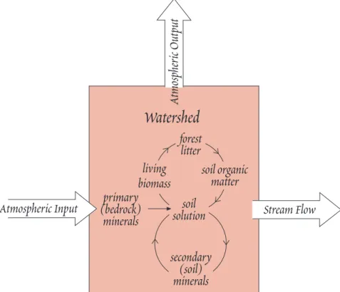
Weathering, Soils, and Biogeochemical Cycling

Weathering is the process by which rock is physically and chemically broken down into relatively fine solids (soil or sediment particles) and dissolved components. The chemical component of weath- ering, which will be our focus, could be more precisely described as the process by which rocks origi- nally formed at higher temperatures come to equilibrium with water at temperatures prevailing a t the the surface of the Earth.

Weathering plays a key role in the exogenic geochemical cycle (i.e., the cycle operating at the sur- face of the Earth). Chemical weathering supplies both dissolved and suspended matter to rivers and seas. It is the prinicipal reason that the ocean is salty. Weathering also supplies nutrients to the bi- ota in form of dissolved components in the soil solution; without weathering terrestrial life would be far different and far more limited. Weathering can be an important source of ores. The Al ore bauxite is the product of extreme weathering that leaves a soil residue containing very high concentrations of aluminum oxides and hydroxides. Weathering, together with erosion, transforms the surface of t h e Earth, smoothing out the roughness created by volcanism and tectonism.

Geochemists are particularly concerned with question of what controls weathering rates. This con- cern arises from both the role weathering plays as a sink for atmospheric CO2 and the variety of an- thropogenic activities that influence weathering rates. Agriculture and harvesting of forests have had a clear impact on erosion, and probably chemical weathering rates as well. Combustion products of fossil fuels released to the atmosphere include nitrates and sulfates that acidify precipitation (Òacid rainÓ). The resulting decrease in pH has had a clear adverse effect on the biota in some locali- ties and may also affect chemical weathering rates. On the other hand, weathering consumes H⁺ and thereby increases pH; in some localities this buffering effect of weathering reactions is sufficient to entirely overcome the effects of acid rain. Understanding the impact of acid rain and the degree to which its effects are mitigated by weathering is an important goal of many weathering studies.

Weathering, and the subsequent precipitation of carbonate in the ocean, also consumes CO2 in reac- tions such as:

CaAl₂Si₂O₈ + H₂CO₃ + 3H₂O ® CaCO₃ + Al₂Si₂O₅(OH)₄

Weathering thus appears to be an important control on the concentration of atmospheric CO2, which is in turn an important control on global temperature and climate. Hence whatever factors control t h e weathering rate may also control climate. What are these factors? In the BLAG (Berner Lasaga and Garrels) model of atmospheric CO2 levels over geological time, Berner et al. (1983) and Berner (1991) assumed that temperature is a strong control on weathering rate, and therefore that there is a nega- tive feedback that controls atmospheric CO2 levels (the higher the atmospheric CO2, the higher t h e global temperature, the higher the weathering rate, and therefore the higher the consumption of atmospheric CO2). Others, including Edmond et al. (1995), have argued that despite the odvious temperature effect on reaction rates, global temperature exerts little control on weathering rates in nature, and that tectonic uplift and exposure of fresh rock has a much stronger influence on weathering rate, and ultimately on global climate.

In previous chapters and sections, we examined many important weathering reactions from thermo- dynamic and kinetic perpectives. In this section, we will step back to look at weathering on a broader scale and examine weathering in nature and the interrelationships among chemical weathering, bio- logical processes, and soil formation. We then discuss in some detail the question of what controls on weathering rates. Finally, we look at the composition of rivers and streams.

Most rock at the surface of the Earth is overlain by a thin veneer of a mixture of weathering prod- ucts and organic matter that we refer to as soil. Most weathering reactions occur within the soil, or a t the interface between the soil and bedrock, so it is worth briefly considering soil and its development.

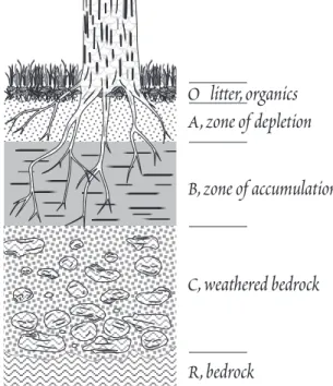
Soil typically consists of a sequence of layers that constitute the soil profile (Figure 13.4). The nature of these layers varies, depending on climate (temperature, amount of precipitation, etc.), vegetation (which in turn depends largely on climate), time, and the nature of the underlying rock. Conse- quently, no two soil profiles will be identical. What follows is a general description of an idealized soil profile. Real profiles, as we shall see, are likely to differ in some respects from this.

Soil Profiles

The uppermost soil layer, referred to as the O horizon, consists entirely, or nearly so, of organic ma- terial whose state of decomposition increases downward. This layer is best developed in forested re- gions or waterlogged soils depleted in O2 where decomposition is slow. In other regions it may be in- completely developed or entirely absent.

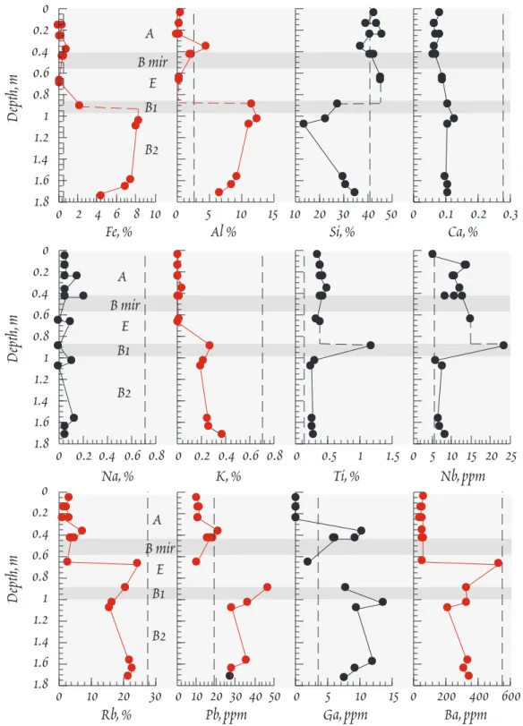
Below this organic layer lies the upper mineral soil, designated as the A horizon or the zone of re- moval, which ranges in thickness from several centimeters to a meter or more. In addition to a vari- ety of minerals, this layer contains a substantial organic fraction, which is dominated by an amor- phous mixture of unsoluble, refractory organic substances collectively called humus. Weathering re- actions in this layer produce a soil solution rich in silica and alkali and alkaline earth cations t h a t percolates downward into the underlying layer. In temperate forested regions, where rainfall is high and organic decomposition slow, Fe and Al released by weathering reactions are complexed by organic

(fulvic) acids and carried downward into the un- derlying layer. The downward transport of Fe and Al is known as podzolization. In tropical re- gions, organic decomposition is sufficiently rapid and complete that there is little available solu- ble organic acid to complex and transport Fe and Al, so podzolization may not occur. As a result, Fe and Al accumlate in the A horizon as hydrous ox- ides and hydroxides. Where leaching is particu- larly strong, the A horizon may be underlain by a thin whitish highly leached, or eluviated, layer known as the E horizon, enriched in highly resis- tant minerals such as quartz. In grasslands and deserts, the production of soluble organic acids is restricted by the availability of water, hence t h e podzolization is limited.

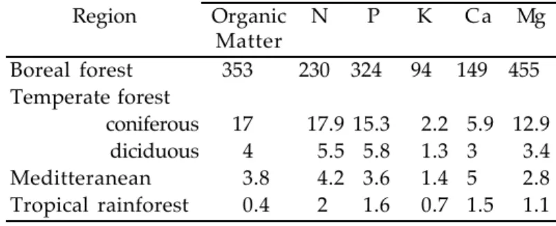
The B horizon, or zone of accumulation or depo- sition, underlies the A horizon. This horizon is richer in clays and poorer in organic matter than the overlying A horizon. Substances leached from the A horizon are deposited in this B horizon. Fe and Al carried downward as organic complexes precipitate here as hydrous oxides and hydrox- ides, and may react with other components in t h e soil solution to form other secondary minerals such as clays. In arid regions where evaporation exceeds precipitation, relatively soluble salts such as calcite, gypsum, and halite precipitate within the soil. Downward percolating water leaches these from the A horizon and concentrates them within in the B horizon. Such calcite layers are known as caliche, and are typically found at a depth of 30 to 70 cm. The clay-rich nature of the B ho- rizon, particularly when cemented by precipitated calcite or Fe oxides, can lead to greatly restrict permeability of this layer. Such impermeable layers are sometimes referred to as hardpan. In tropi- cal regions, where weathering is intense and has continued for millions of years in the absence of dis- turbances such as glaciation, the soil profile maybe up to 100 m thick. Because of the absence of podzolization, there is often little distinction between the A and B horizons. Base cations are nearly completely leached in tropical soils, leaving a soil dominated by minerals such as kaolinite, gibbsite, and Fe oxides. Such soils are called laterites. In the most extreme cases, SiO2 maybe nearly com- pletely leached as well, leaving a soil dominated by gibbsite. The ratio of SiO2 to Al2O3 + Fe2O3

(collectively called the sesquioxides) is a useful index of the intensity of weathering within the soil as well as to the extent of podzolization. Typical values for the A and B horizons of several climatic regions are summarized in Table 13.2. Often, seperate layers can be recognized within the B and t h e other horizons and these are designated B1, B2, etc. downward.

The C horizon underlies the B horizon and directly overlies the bedrock. It consists of partly weathered rock, often only coarsely frag-

mented, and its direct weathering prod- ucts. Very often it consists of saprolite, rock in which readily weatherable sili- cates have been largely or wholy re- placed in situ by clays and oxides, but tex- tures and structures are often sufficiently well preserved that the nature of t h e original parent maybe recognized. This

O litter, organics A, zone of depletion B, zone of accumulation

C, weathered bedrock

R, bedrock

Figure 13.4. Soil profile, illustrating the O, A, B, and C horizons described in the text. Not a l l soils comform to this pattern.

Table 13.2. SiO₂/(Al₂O₃ + Fe₂O₃) Ratios of Soils

A horizon B horizon

Boreal 9.3 6.7

Cool-temperate 4.07 2.28

Warm-temperate 3.77 3.15

Tropical 1.47 1.61

From Schlesinger (1991).