Surrogate models for discrete optimization problems

(1)

O PTIMIZATION P ROBLEMS

Dissertation

zur Erlangung des Grades eines

D OKTORS DER I NGENIEURWISSENSCHAFTEN

der Technischen Universität Dortmund an der Fakultät für Informatik

von

M ARTIN Z AEFFERER

Dortmund

2018

(2)

Tag der mündlichen Prüfung:

19. Dezember 2018 Dekan:

Prof. Dr.-Ing. Gernot A. Fink Gutachter:

Prof. Dr. Günter Rudolph, Technische Universität Dortmund

Prof. Dr. Thomas Bartz-Beielstein, Technische Hochschule Köln

(3)

This thesis was some years in the making. During these years, it profited from the indispensable support (moral and professional) of many people. Hence, I express my gratitude to my

• supervisor Prof. Dr. Thomas Bartz-Beielstein, who triggered my interest into this research field. He has since been a strong support and a source of motivation for my scientific work.

• supervisor Prof. Dr. Günter Rudolph. Our discussions always provided new impulses, and opened up questions that I might not have touched on otherwise.

• mentor Prof. Dr. Gabriele Kern-Isberner, for helpful discussions on work-life- balance, ideation, and systematic approaches of research.

• colleagues, who often discussed potential applications and connected research (especially Oliver, Jörg, Martina, Andreas, Frederik), gave support for the com- putational experiments and related technical aspects (Sebastian, Oliver, Andreas), proofread drafts (Frederik), gave feedback on my articles and presentations, helped me to see my research from a different view, and/or helped to reduce my workload in the final phase of my thesis.

Thanks to all of you: Beate Breiderhoff, Sowmya Chandrasekaran, Andreas Fis- chbach, Oliver Flasch, Martina Friese, Lorenzo Gentile, Dimitri Gusew, Dani Irawan, Christian Jung, Patrick Koch, Sebastian Krey, Olaf Mersmann, Steffen Moritz, Boris Naujoks, Quoc Cuong Pham, Stefanie Raupach, Margarita Re- bolledo, Frederik Rehbach, Viktoria Schaale, Jörg Stork, Katya Vladislavleva, and Svetlana Zakrevski.

• parents Monika and Rolf Zaefferer, for the patient support and encouragement

during these years.

(4)

4 CONTENTS

Chapter 1 Introduction

In real-world optimization, it is often expensive to evaluate the quality of a candidate solution. The costs may be due to run-time of a complex computer simulation, time required for a laboratory experiment, expensive material for building a prototype, or cost of operator work hours. In these cases, it is desirable to evaluate as few candidate solutions as possible.

Surrogate Model-Based Optimization (SMBO) techniques try to achieve this by shift- ing the evaluation load from the expensive experiment to a surrogate model. This model is expected to be a cheap-to-compute abstraction of the real-world problem.

1.1 Incentive

Surrogate modeling has been firmly established in the field of continuous optimization with real-valued parameters [136, 257, 232, 137, 26]. Nevertheless, many optimiza- tion problems are not continuous. Rather, search spaces are often spanned by discrete variables or are based on complex structures such as graphs. In fact, one of the first ex- periments with evolution strategies dealt with an expensive and discrete optimization problem: Schwefel’s optimization of a two-phase jet nozzle [225, 149]. Here, the ex- perimental restrictions imposed a discrete search space: 239 available nozzle segments could be combined to form different nozzle shapes [225].

More recent application examples can be found in the fields of mechanical engineer- ing [254, 11, 231, 42, 244, 245], aerospace engineering [131], chemical engineer- ing [104, 118, 108], bioinformatics [71, 212], operations research [85, 121, 191, 192, 190, 174] or data science [235] and algorithm tuning [126, 128, 34, 33, 241, 246, 80, 125, 38, 198, 72, 161]. In these problem domains, combinatorial data structures (e.g., categorical variables, sequences, strings, or graphs) have to be optimized, and the eval- uation procedures are often very expensive.

Many of these examples are quite recent developments; others are not relying on sur-

rogate models at all. Several works in recent years suggested that this field has not

been investigated in depth and poses a challenge to SMBO algorithms [257, 232, 179,

137, 9, 110]. So what is the reason for this, and what is really missing? Clearly, a large

(10)

10 1.2. OBJECTIVE

variety of model-free optimization techniques for black-box problems is readily avail- able, e.g., evolutionary algorithms or other metaheuristic optimization algorithms [43].

It seems that we lack suitable surrogate models to apply techniques like evolution- ary algorithms to expensive, discrete problems. Moreover, the interdisciplinary nature of this research field (engineering applications, combinatorial optimization, machine learning, evolutionary computing) causes additional complications in practice.

It is the aim of this work to fill this void. Based on the state of the art in surrogate modeling, we attempt to establish the missing links in combinatorial, discrete, and mixed variable SMBO. We focus on developing or improving suitable models.

1.2 Objective

The main objective of this thesis is to develop methods for solving the optimization problem

min

x∈X

f (x),

where X is a nonempty set (the search space). An element x of that set represents a candidate solution of the optimization problem. The objective function f(x) is usually assumed to be expensive (with respect to money, time or material resources) and a black-box. Here, the term “black-box” implies that knowledge about the objective function f (x) can only be obtained by evaluating it, no further prior knowledge is available. At the same time, the cost of the overall optimization procedure is dominated by the number of evaluations of f(x). This causes the main complexity of this problem type: the black-box nature of the problem necessitates a certain amount of function evaluations, yet the cost of these evaluations imposes a strict limit on their number.

This motivates the use of surrogate models.

An important premise for this thesis is the nature of the solutions x. Surrogate model- ing is well-established for x ∈ R

^m

, where m indicates the dimensionality of the search space, that is, the number of real-valued parameters. We aim for a more general case, where x is allowed to have a more complex structure. Most importantly, it may be of a combinatorial or discrete nature, e.g., permutations, strings, graphs, or mixtures of representations. In this case, relatively few approaches have been investigated in the literature. There is only one restriction required for most of the methods described in this thesis. A kernel function k(x, x

⁰

) has to be available, which comprehends some measure of similarity or distance. This implies that k(x, x

⁰

) can be computed for any x, x

⁰

∈ X .

If such a kernel is available, the methods developed in this thesis are applicable to any kind of continuous, mixed, discrete, or combinatorial solution representation. In particular, this thesis deals with the following solution representations:

• Continuous variables are used in various illustrative examples, and are consid- ered in Chapter 2.

• Permutations are used as a frequent test case in Chapters 5 to 8.

(11)

• Binary variables are used in experiments in Chapter 5.

• Strings are briefly considered in Section 7.4.4.

• Tree structures are considered in Section 9.1, in the context of genetic program- ming and symbolic regression.

• Graphs that encode hierarchical dependencies of variables are considered in Sec- tion 9.2.

• Categorical variables are considered in an application in Section 9.3.

1.3 Synopsis

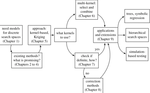
A graphical overview of this thesis is given in Fig. 1.1. In the following, we extend this overview with more details.

Firstly, we provide the required background on black-box optimization methods and surrogate modeling in Chapter 2. This initial overview mostly deals with methods from the continuous domain. Chapter 3 extends this with an overview of surrogate models in the discrete domain. This provides a review of the state of the art, to give a clear indication of what other approaches exist. Our further work heavily relies on kernels, which are discussed in Chapter 4.

Based on the introduced background, Chapter 5 deals with the core methods of this thesis: a Kriging model for discrete search spaces based on appropriate distances or kernels. Kriging is a frequently used surrogate model for continuous problems that re- gresses or interpolates data based on measures of correlation, or kernel functions [93].

need models for discrete search spaces

(Chapter 1)

existing methods?

what is promising?

(Chapters 2 to 4) approach:

kernel-based, Kriging (Chapter 5)

what kernels to use?

multi-kernel:

select and combine (Chapter 6)

check if definite, how?

(Chapter 7)

correction methods (Chapter 8)

applications and extensions

(Chapter 9)

trees, symbolic regression

hierarchical search spaces

simulation- based testing

no yes

Figure 1.1:

A brief overview of this thesis, following the main lines of the investigation.

(12)

12 1.4. PUBLICATIONS

The intuitive idea is to change the underlying kernel, thus adapting Kriging to the dis- crete data types investigated in this thesis. The rationale behind this is explained, and a first set of experiments is investigated as a proof of concept.

As the experiments show, it is not always clear which kernel to use for a specific ap- plication. Hence, we investigate methods that select or combine kernels in Chapter 6.

These multi-kernel methods mostly employ the following concepts: linear relation- ships between kernels and observations, likelihoods, and cross-validation. Our results indicate that it is crucial to employ multi-kernel methods, to avoid poor algorithm per- formance.

However, not every kernel fulfills the requirements of the modeling techniques. Im- portantly, kernels are expected to be definite. An indefinite kernel may deteriorate the accuracy of the model. Even worse, an indefinite kernel may sometimes produce no feasible model at all. Hence, it is important to know whether a kernel is definite. In Chapter 7, we propose a novel, empirical approach to that end. A search procedure either tries to find indefinite cases by random sampling or by optimizing a critical eigenvalue.

Once a kernel is determined to be indefinite, appropriate counter-measures have to be taken to avoid performance losses. Chapter 8 demonstrates how Kriging models can be enabled to deal with indefinite kernels. Most importantly, transformations of the eigen- spectrum are employed to correct definiteness. This idea is borrowed from the field of support vector learning. Additionally, we suggest further correction approaches and condition repair methods that allow transplanting these approaches to Kriging models.

Finally, in Chapter 9, we explore whether our methods are able to handle problems that are more complex. A tree-based symbolic regression task and hierarchical search spaces are investigated. Importantly, this is extended by a discussion of algorithm benchmarking. We propose a test function generator based on a data-driven Kriging simulation. This generator produces diverse test functions, which are able to reflect the behavior of real-world problems.

This work is finalized in Chapter 10, by giving an overall summary, providing some advice for practitioners and outlining future research directions.

To supplement these considerations, the appendix collects further odds-and-ends, in- cluding tools for the statistical analysis of results (Appendix A), a description of spe- cific kernels employed in the thesis (Appendix B), a description of the employed vari- ation operators (Appendix C), and additional figures (Appendix D).

1.4 Publications

Significant parts of this work are based on material that has previously been published or is being prepared for publication during the writing of this thesis. Of significance are the following documents: [273, 271, 264, 26, 266, 268, 270, 272].

All these works have been extended, rewritten, and restructured in some form before

their inclusion into this thesis. The rewriting and restructuring were mostly aimed to

(13)

increase the clarity, to unify notation and terminology, and put the described contri- butions in the overall context of this thesis. In most cases, this includes a revision or extension of the experiments. In the following, the changes are briefly outlined.

If not otherwise specified, these publications are in large parts a contribution of the author of this thesis. This is not intended to underrate the contributions of the co- authors, who provided inspiration to some of the presented ideas, helped to improve the writing quality, and gave support for the experimental procedures and analysis of these studies. In the following, we discuss each publication. For the sake of clarity, these remarks are repeated at the start of the respective sections or chapters.

Chapter 3 is partly based on the article “Model-based Methods for Continuous and Discrete Global Optimization” by Bartz-Beielstein and Zaefferer [26]. This includes many text elements that are taken verbatim from that publication. In the article, the discussion of continuous optimization methods was mostly contributed by Thomas Bartz-Beielstein. The part that is relevant to this chapter was mostly contributed by the author of this thesis. The survey was rewritten, restructured, and expanded. To a lesser extent, a few considerations have been taken from the article “Efficient Global Optimization for Combinatorial Problems” by Zaefferer et al. [273].

In less detail, some of the terms and definitions from Chapter 4 have already been discussed in Section 2 of “An Empirical Approach for Probing the Definiteness of Kernels” by Zaefferer et al. [266]. Hence, there is some overlap with that section. We added more details, including an illustrative motivation of the kernel trick.

Chapter 5 is partially based on the article “Efficient Global Optimization for Combi- natorial Problems” by Zaefferer et al. [273]. Occasionally, text elements have been adopted verbatim from that publication. Overall, the text was significantly rewritten and extended before its inclusion into this thesis. We also added an illustrative exam- ple. The described experiments were repeated in a more thorough way. This included a more flexible, self-adaptive evolutionary algorithm, a broader set of test functions, and a parameter sensitivity study.

Chapter 6 is based on the article “Distance Measures for Permutations in Combinato- rial Efficient Global Optimization” by Zaefferer et al. [271], with similar extensions as in Chapter 5. Some text elements have been adopted verbatim from the original con- tribution. The content of the publication been extended significantly. Firstly, several additional methods for dealing with multiple kernels are discussed, including a more comprehensive explanation of the original ideas. Secondly, a more thorough experi- mental study now includes these methods as well as additional distance measures and test functions. Furthermore, the results are subject to a more in-depth analysis.

Chapter 7 is based on the article “An Empirical Approach for Probing the Definiteness of Kernels” by Zaefferer et al. [266]. The material was revised to embed it into the context, notation, and structure of this thesis. Otherwise, a majority of the text has been adopted verbatim from the original document. The experiments and analysis were not changed.

Chapter 8 is based on the article “Efficient Global Optimization with Indefinite Ker-

nels” by Zaefferer et al. [264]. It has been extended and rewritten. Some parts are

(14)

14 1.4. PUBLICATIONS

taken verbatim from the original publication. An illustration with a one-dimensional example was added. Further, the experimental setup was extended to deal with test problems that are more varied and of a higher dimension. Correspondingly, the ex- perimental analysis had to be adapted. The remarks on non-stationarity are also not part of the original article. Finally, some additional repair methods based on a linear combination and a nearest-neighbor approach were added.

Chapter 9 is largely based on three publications [272, 270, 268].

Section 9.1 is based on the article “Linear Combination of Distance Measures for Sur- rogate Models in Genetic Programming” by Zaefferer et al. [272]. Especially in the problem description, the description of the distances, and the experimental setup, ma- jor parts were taken verbatim from the original article. Otherwise, the text was revised and the description of the distances and the analysis were supplemented with a dis- cussion of definiteness. This includes additional experimental results with definiteness correction methods. The analysis was extended, especially with visualizations.

Section 9.2 is based on the article “A First Analysis of Kernels for Kriging-based Opti- mization in Hierarchical Search Spaces” by Zaefferer and Horn [270]. It was prepared in a coequal cooperation with Daniel Horn, who especially contributed to the statistical and visual analysis of the experimental investigation. Since this article was written in equal parts by both of its authors, it is not discussed entirely. We discuss the kernels contributed by the author of this thesis in more detail (with few verbatim adoptions) and briefly summarize the experimental results. An additional kernel (Wedge-kernel) is proposed.

Section 9.3 is mostly based on “Simulation Based Test Functions for Optimization Al- gorithms” by Zaefferer et al. [268]. The text is in parts taken verbatim from that pub- lication. However, it was largely rewritten and extended to 1) give a clearer motivation supported by visualizations, 2) add some additional remarks on related approaches, 3) discuss the advantages and disadvantages in a more structured way, 4) provide more illustrative examples to explain how the test function generator works, and 5) show results from an additional experiment with a random forest model.

In addition to these main chapters, a few excerpts regarding the description of kernels, distances, and variation operators described in the appendix are taken from already mentioned publications [273, 271, 264, 266].

Finally, the author of this thesis was involved in several research projects and studies

that are not directly related to the core issues that are discussed here. Hence, they are

not included in these deliberations. In particular, some of these publications discussed

interesting applications of SMBO algorithms in fields like process optimization [269],

algorithm tuning [265, 267], and mechanical engineering [143, 27]. While none of

these applications considered discrete or combinatorial problems, they provided an

initial motivation and foundation for this work.

(15)

Part I

Background and State of the Art

(16)

16

Chapter 2 Continuous Methods for Expensive Black-box Optimization

The modeling and optimization methods developed in this thesis are based on estab- lished techniques in the field of vector-valued, continuous optimization. The founda- tions of methods for expensive, black-box optimization problems are introduced in the following. In this chapter, a candidate solution x is considered to be an m-dimensional real-valued vector in the search space X ⊆ R

^m

, and f (x) is a continuous, expensive, black-box function.

2.1 Evolutionary Algorithms

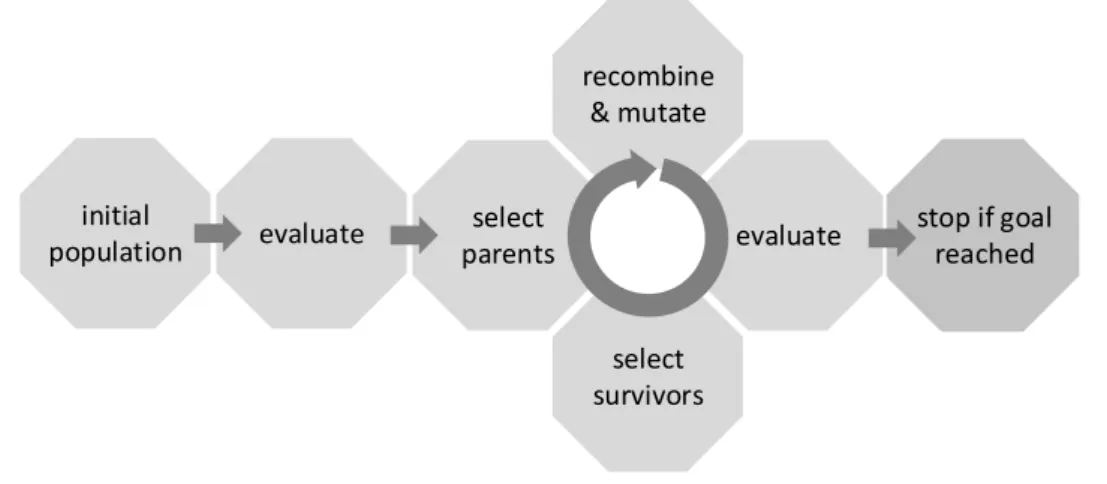
One prominent class of solvers for black-box optimization problems are Evolutionary Algorithms (EAs) [226, 208, 13, 82, 23]. These algorithms transfer the concept of natural evolution to numerical optimization. EAs combine selection, mutation, and re- combination of candidate solutions iteratively, as outlined in Algorithm 1 and Fig. 2.1.

The following list summarizes some of the most important aspects of an EA.

• Candidate solutions x ∈ X are called individuals.

• A population X ⊂ X is a set of individuals.

• The objective function f (x) is called the fitness function. The output of that function is the fitness of an individual x.

• A recombination operator is a function that creates one or more offspring (new

individuals, denoted X

⁰

in Algorithm 1), using information of two or more par-

ents (old individuals). For instance, two parents x

⁽¹⁾

, x

⁽²⁾

can be recombined

by taking the average in each dimension: x

⁰

= (x

⁽¹⁾

+ x

⁽²⁾

)/2. This particular

example is called intermediate crossover.

(17)

stop if goal reached evaluate

select survivors recombine

& mutate

select parents evaluate

initial population

Figure 2.1:

A simplified schema of how an evolutionary algorithm evolves better solutions.

• Mutation operators induce slight changes in offspring. For example, a normally distributed error is added to an individual x

⁰

= x

⁰

+ z, where z is a vector of independent samples from the normal distribution, i.e., z

_i

∼ N (µ, σ

²

), with µ = 0. Here, N (µ, σ

²

) denotes the normal distribution with mean µ, and variance σ

²

. In this context, σ

²

is also called the step-size, step-length, or mutation strength.

• A selection mechanism is required to select which of the individuals in a popula- tion are chosen as parents (parent selection). Furthermore, a subset of the parent population and the offspring needs to be selected for the next iteration (survivor selection). The selection process usually depends on the fitness (or fitness ranks).

One important aspect of EAs is the configuration of their parameters, e.g.,

• the population size n

_pop

(the size of the set X),

• the number of generated offspring n

_off

(the size of the set X

⁰

),

• the choice of mutation operator (Line 11 of Algorithm 1),

• the choice of recombination operator (Line 10 of Algorithm 1),

• the choice of selection operators (Lines 9 and 19 of Algorithm 1), and

• parameters of the operators (e.g., step-sizes or selection probabilities).

All these parameters can influence the performance of an EA. A good configuration

may be critical to the success of the algorithm. This implies a meta-optimization prob-

lem: the optimization of the algorithm’s performance. Optimal values depend not

only on the algorithm but also on the problem. For example, highly multimodal prob-

lems may require a larger population size, whereas a small population size is more

(18)

18 2.1. EVOLUTIONARY ALGORITHMS Algorithm 1 Evolutionary algorithm.

1:

function EA(f(x), init(), select() mutate(), recombine(), terminate())

2:

X =init() ; . create initial population with X ⊂ X

3:

n = |X|; . size of the population

4:

for j = 1 to n do

5:

y

_j

= f(x

^(j)

); . evaluate fitness of each individual

6:

end for

7:

y =

y

₁

. . . y

_n

T

;

8:

while not terminate() do

9:

X

_parent

= select (X, y); . parent selection

10:

X

⁰

= recombine (X

_parent

); . recombination

11:

X

⁰

= mutate (X

⁰

); . mutation

12:

n = |X

⁰

|;

13:

for j = 1 to n do

14:

y

_j⁰

= f (x

⁰_j

); . evaluate fitness of offspring

15:

end for

16:

y

⁰

=

y

⁰₁

. . . y

⁰_n

T

;

17:

X = X ∪ X

⁰

; . add offspring to population

18:

y =

y y

⁰

;

19:

X, y = select (X, y); . survival selection

20:

end while

21:

end function

efficient for a unimodal problem. Therefore, to understand and improve an EA’s per- formance, its parameters have to be considered. In this context, we will call them meta-parameters. Two approaches are important in that respect.

Firstly, parameter tuning can solve this meta-optimization problem via some optimiza- tion algorithm. This algorithm can itself be an EA, or some more sophisticated method, such as sequential parameter optimization [24, 20]. Tuning not only improves results, but also enables a fair comparison between the tuned algorithms.

The second approach is parameter control [227, 81]. This includes a process into the al- gorithm that adapts the algorithm parameters during its runtime. One classical example is the so-called one-fifth rule suggested by Rechenberg [208]. This rule was devised for the step-size adaptation of the (1+1)-Evolution Strategy (ES) on two unimodal fitness functions. The (1+1)-ES operates with a single parent and a single offspring. The rule states that the step-size should be increased if more than one trial in five iterations yield a better fitness, and it should be decreased if fewer improvements are observed. An- other parameter control approach is self-adaptation. The term self-adaptation implies that the algorithm parameters are attached to the parameters x of the objective func- tion [81]. That means, x

^∗

=

x x

_meta

, where x

_meta

are meta-parameters of the EA (or

(19)

more specifically, all parameters controlled by self-adaptation), x are the parameters of the underlying fitness function, and x

^∗

is their concatenation. Consequently, some of the EA’s parameters may vary between different individuals. By processing x

^∗

instead of just x, the EA can search for the optimum of the fitness function and the solution of the meta-optimization problem simultaneously.

Parameter control is not without problems and may still require tuning. Firstly, it has been shown that self-adaptation may lead to premature convergence [217]. Secondly, most adaption schemes introduce new parameters, such as learning rates. We refer to these parameters as learning parameters. Still, it is usually argued (but not necessarily guaranteed) that algorithms should be less sensitive to learning parameters [81].

For example, Algorithm 2 represents a self-adaptation scheme that is used in this the- sis. This self-adaptation process is applied to the parent individuals, before an offspring is created by recombination and mutation. Therefore, the process is placed between Lines 9 and 10 of Algorithm 1. For the adaptation of real-valued meta-parameters, we use an approach similar to that in the mixed-integer ES (MIES) [84, 163]. In addition to the MIES, we also consider categorical meta-parameters, e.g., the choice of variation operators. To that end, we use a rather simple concept: If offspring are generated by recombination, the categorical meta-parameter is chosen randomly from each parent.

This is also called dominant crossover. Afterwards, mutation may change a categor- ical meta-parameter with probability p

_s

. If a mutation is triggered, the adaptation is performed via a uniform random sample from all values (except for the current value).

Algorithm 2 Self-adaptation of an EA’s meta-parameters, placed between Lines 9 and 10 of Algorithm 1.

1:

function

SELF

-

ADAPT

(parent population X

^∗

and learning parameters τ , p

_s

)

2:

for all x

^∗

∈ X

^∗

do

3:

for all real-valued x

_meta

∈ x

^∗

do . e.g., mutation rate

4:

recombine: intermediate crossover;

5:

mutate: x

_meta

= x

_meta

exp(τ z) with z ∼ N (0, 1);

6:

end for

7:

for all categorical x

_meta

∈ x

^∗

do . e.g., variation operators

8:

recombine: dominant crossover; . choose randomly from parents

9:

mutate: uniform random sample, with probability p

_s

;

10:

end for

11:

end for

12:

return X

^∗

13:

end function

In Algorithm 2, the learning rate τ and the probability p

_s

are new learning parame-

ters introduced by the self-adaptation scheme. Here, these parameters are defined as

scalars, but they can as well be specified as vectors to encode different rates or proba-

bilities for each of the controlled meta-parameters.

(20)

20 2.2. SURROGATE MODEL-BASED OPTIMIZATION

Overall, EAs have several advantages that make them a promising choice for the black- box problems considered in this thesis:

• EAs require no additional information about the search space, such as gradients.

• Due to their population-based, stochastic nature, EAs have the potential to es- cape local optima.

• EAs can be easily adapted to different data structures, and are in fact widely used in continuous as well as discrete optimization.

• Although a well-performing EA may require significant parameter tuning effort, little domain knowledge is required for the general setup of an EA.

However, EAs have a crucial feature that puts them at odds with one main constraint of the problems considered in this thesis. EAs require many fitness evaluations, which are often expensive to evaluate in case of real world optimization problems. Hence, we need tools for the efficient optimization of expensive, discrete problems with EAs.

In the remainder of this thesis, we focus on surrogate model-based optimization tech- niques that provide sophisticated tools for solving these problems.

2.2 Surrogate Model-based Optimization

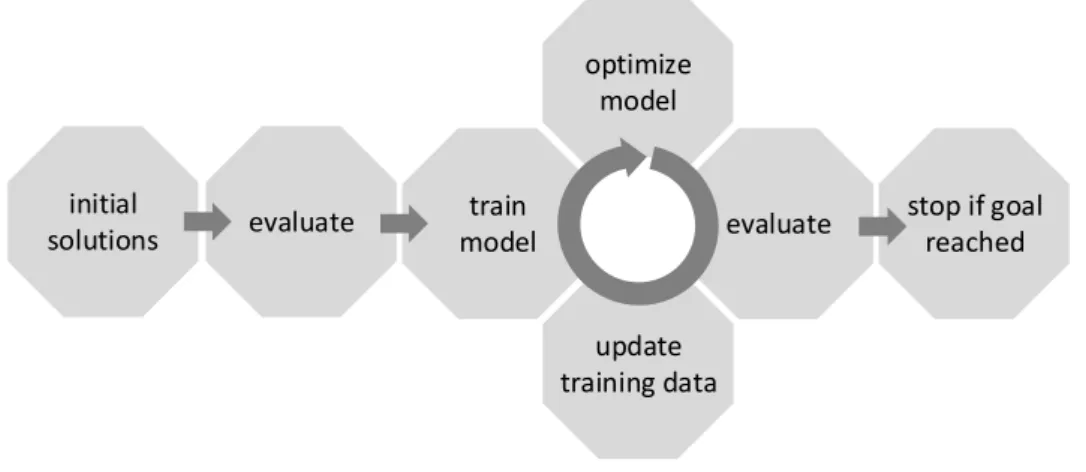
Algorithm 3 defines a typical SMBO algorithm. A simplified schema of this algo- rithm is depicted in Fig. 2.2. Similar algorithms are used throughout this thesis. In the SMBO algorithm, f(x) is the expensive objective function, init() generates an experimental design (a set of initial candidate solutions), model() is a function that trains data-driven surrogate models, optimizer() is an optimization algorithm that optimizes the model based on some infill criterion, and terminate() checks whether the algorithm should stop (e.g., based on a budget of evaluations of f ).

update training data

stop if goal reached evaluate

optimize model

train model evaluate

initial solutions

Figure 2.2:

A simplified schema of how an SMBO algorithm searches for better solutions.

(21)

Algorithm 3 A typical SMBO algorithm

1:

function SMBO(f (x), init(), model(), optimizer(), infill, terminate())

2:

X =init() ; . create initial design with X ⊂ X

3:

n = |X|;

4:

for j = 1 to n do

5:

y

_j

= f(x

^(j)

); . evaluate design

6:

end for

7:

y =

y

₁

. . . y

_n

T

;

8:

while not terminate() do

9:

M = model (X, y); . create / update the model

10:

x

⁰

= optimizer(M ,infill); . determine promising candidate

11:

y

⁰

= f (x

⁰

); . evaluate candidate

12:

X = X ∪ {x

⁰

}; . add candidate to data set

13:

y =

y y

⁰

; . add objective function value of candidate

14:

end while

15:

end function

The init() algorithm may create, e.g., Latin hypercube designs [172] or other (prefer- ably space-filling) designs.

The model() algorithm may employ, e.g., linear regression models, Random Forests (RF), Radial Basis Function Networks (RBFN), Artificial Neural Networks (ANN), Support Vector Machines (SVM), or other data-driven regression models [126, 137].

These models are assumed to be cheaper to evaluate than the expensive objective func- tion f(x). One of the more frequently used surrogate models is Kriging [220, 93]. It is in the focus of this thesis and is introduced in more detail in Section 2.3.

The optimizer() algorithm may be, e.g., the EA described in Algorithm 1, or any other global optimization algorithm. The optimizer can either directly optimize the prediction of the model, or else it could optimize a so-called infill criterion that is derived from the model [93] (cf. Section 2.4). In essence, the optimizer can thus avoid evaluating the expensive fitness function directly. Instead, the EA repeatedly optimizes a surrogate model that becomes increasingly accurate during the optimization run.

For a more detailed review of SMBO techniques, we refer to the literature [136, 257, 232, 137, 26]. One important link between EAs and SMBO is the pre-selection approach of the metamodel-assisted evolution strategies discussed by Emmerich et al. [83]. SMBO algorithms find application in many domains. Besides engineering de- sign [93], algorithm tuning is a frequent area of application. The sequential parameter optimization approach [24, 20] mentioned in Section 2.1 is one important framework in this context.

Sometimes, SMBO problems can become multi-objective. That implies, potentially

conflicting goals may have to be satisfied by the optimization procedure. We focus

(22)

22 2.3. INTRODUCTION TO KRIGING

on single-objective problems, but the models discussed in this thesis may as well be applied to multi-objective problems. For more details on such considerations, we refer to a recent survey by Chugh et al. [63].

2.3 Introduction to Kriging

The popularity of Kriging (also known as Gaussian process regression) in the field of SMBO is based on its flexibility and predictive accuracy. In addition, it provides an estimate of its own uncertainty. The latter feature is especially useful in SMBO algorithms, as it is crucial for the computation of many infill criteria. The foundations of these ideas are the seminal works by Mockus et al. [175], Sacks et al. [220], and Jones et al. [140]. A very comprehensive description of Kriging-based optimization is given by Forrester et al. [93], whose work is also an important basis for the following remarks and equations.

2.3.1 Kriging Model

We assume that we have some data set X = {x

⁽¹⁾

, . . . , x

⁽ⁿ⁾

} of n ∈ N samples, each sample being an m-dimensional real-valued x ∈ R

^m

. The corresponding observations for each sample are represented by the vector y ∈ R

ⁿ

. Kriging can make powerful predictions with the (on the first glimpse) simple model:

y

_i

= µ +

_i

Importantly, Kriging assumes that the observations y are realizations of a stochastic process where the errors

_i

are spatially correlated. Two nearby observations should have a similar error. Thus,

_i

is clearly dependent on the sample location x, and we can write (x

⁽ⁱ⁾

). Errors are considered to be positively correlated if the distance between two sample locations is small. Correlation goes to zero with increasing distance. This relationship between the correlation of the errors and the distance of the samples can be modeled with, e.g.,

k(x, x

⁰

) = exp −

m

X

i=1

θ

_i

|x

_i

− x

⁰_i

|

^pⁱ

!

, (2.1)

where x

_i

∈ R is the i-the component of the vector x. The function given in Eq. (2.1) is one important example of a correlation function, or kernel. Other correlation func- tions can be defined, but they would usually have to satisfy some important criteria.

For instance, they should approach zero for large distances, they should yield one if

x = x

⁰

, and they should usually be positive semi-definite (definiteness is discussed in

Chapters 4, 7 and 8). A matrix that collects pairwise correlations between errors of all

observations y at locations X is the correlation matrix (or kernel matrix) K.

(23)

p =1 q =1 p =2

q =1 p =2 q =5 p =1

q =5

0.00 0.25 0.50 0.75 1.00

0.0 0.5 1.0 1.5 2.0 2.5

x - x ¢

k( x , x' )

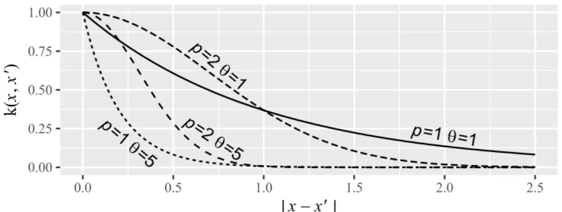
Figure 2.3:

An illustrative example of how the correlation function in Eq.

(2.1)

behaves with different sets of parameters. The plot shows the correlation in relation to the distance (absolute difference) of two real-valued, scalar samples.

The correlation function in Eq. (2.1) has two parameters for each dimension of the search space, θ

_i

and p

_i

. The interpretation of the parameters θ

_i

and p

_i

can be best understood when looking at the example in Fig. 2.3. The parameter θ

_i

influences how fast the function decays to zero. The parameter p

_i

controls the smoothness, i.e., how acute the curve is when the distance approaches zero.

The values of these parameters can be determined by Maximum Likelihood Estimation (MLE) [93]. With MLE, parameters are chosen so that the observed data has the largest likelihood, given the specified model. The likelihood function of the Kriging model is based on the probability density function of a multivariate normal distribution,

pdf

_MVN

(y) = 1

(2π)

^n/2

|C|

^1/2

exp

− 1

2 (y − 1µ)

^T

C

⁻¹

(y − 1µ)

,

where 1 is a vector of ones. The stationary covariance matrix C is related to the correlation matrix K with

C = σ

²

K. (2.2)

This yields the likelihood function

L((X)|µ, σ, θ, p) = 1

(2πσ

²

)

^n/2

|K|

^1/2

exp

− (y − 1µ)

^T

K

⁻¹

(y − 1µ) 2σ

²

. (2.3) Here, µ and σ are also parameters to be determined by MLE. To determine all param- eters (θ, p, σ, µ) by MLE, the partial derivatives of the likelihood function have to be set to zero. The partial derivatives yield closed-form solutions for µ and σ

²

,

ˆ

µ = 1

^T

K

⁻¹

y

1

^T

K

⁻¹

1 ,

(24)

24 2.3. INTRODUCTION TO KRIGING

and

ˆ

σ

²

= (y − 1 µ) ˆ

^T

K

⁻¹

(y − 1 µ) ˆ

n .

By taking the logarithm, substitution of µ ˆ and σ, and subsequent removal of constant ˆ terms, Eq. (2.3) becomes the so-called concentrated log-likelihood function:

con(ln(L)) = − n

2 ln(ˆ σ

²

) − 1

2 ln(|K|).

This function is used to find the remaining parameters of the correlation function.

However, an algebraic, closed-form solution is not available. Instead, numerical op- timization is required to maximize the concentrated log-likelihood with respect to the remaining parameters. This can be done with classical optimization methods, or with population-based methods, like EAs, to allow for a global search.

2.3.2 Kriging Prediction

With the equations discussed above, we can derive the necessary parameters of a model that describes the observed training data. But how can this model be used to generate predictions with respect to a new sample x

^∗

? In the following, the basic idea of predic- tion with Kriging is explained. Forrester et al. give a more detailed derivation of the formulas [93] that we use as a basis for this description.

The unknown function value of a new solution is denoted as y. Determining this value ˆ is denoted as prediction. The core idea is to add the new solution to the set of existing solutions. This yields the augmented vector of observations y

_aug

=

y

^T

y ˆ

T

. Then, we treat y ˆ like a model parameter. That is, we maximize the likelihood function with respect to y. To that end, the vector of correlations between a new sample ˆ x

^∗

and the set of training samples X is, k =

(k(x

⁽¹⁾

, x

^∗

), ..., k(x

⁽ⁿ⁾

, x

^∗

)

^T

. This is used in the augmented correlation matrix K

_aug

=

K k k

^T

1 . K

_aug

, y

_aug

, and all earlier determined model parameters are substituted into the likelihood function in Eq. (2.3).

Maximizing the terms of Eq. (2.3) depending on y ˆ yields the predictor ˆ

y(x

^∗

) = ˆ µ + k

^T

K

⁻¹

(y − 1 µ). ˆ (2.4)

2.3.3 Uncertainty Estimate

An important feature of Kriging is that it also provides an estimate of its own local uncertainty, or its prediction error. Roughly speaking, if the new sample x

^∗

has a large distance to the training data, the uncertainty of the predicted value is also large.

Typically, the uncertainty also increases if the model gets more rugged or active in the

(25)

respective region (i.e., large rates of change). The uncertainty of the prediction can be estimated with [220, 93]

ˆ

s

²

(x

^∗

) = ˆ σ

²

(1 − k

^T

K

⁻¹

k). (2.5) Kriging is not the only modeling tool that can produce uncertainty estimates. For ex- ample, uncertainties could always be estimated by training models with subsets of the data (e.g., cross-validation). However, stochastic models, like Kriging, produce these estimates quite naturally, with little additional effort, and impose important proper- ties on the uncertainty estimates. For instance, if no noise is modeled, the uncertainty estimate goes to zero with decreasing distance to a training data sample. Uncertain- ties estimated by cross-validation would be non-zero at the training samples. The importance of the uncertainty estimate and its properties in model-based optimization becomes more clear in Section 2.4.

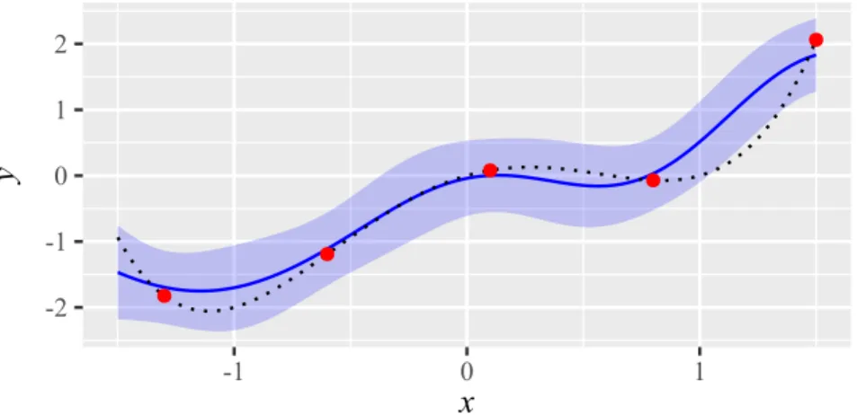
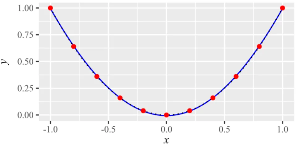
Example 2.3.1. To demonstrate the predictor and uncertainty estimate of a Kriging model, we consider the simple function

y = f(x) = x

⁴

− 2x

²

+ x,

with x ∈ R . The function has been sampled at X = {−1.3, −0.6, 0.1, 0.8, 1.5}. The corresponding observations are y ≈

−1.82 −1.19 0.08 −0.07 2.06

T

. We fix p = 2 for the sake of simplicity and the maximum likelihood estimate of the remaining kernel parameter is θ ≈ 1.97. We provide a plot of the resulting predictor in Fig. 2.4.

-2 -1 0 1 2

-1 0 1

x

y

Figure 2.4:

The prediction

y(x)ˆ

of a Kriging model (blue solid line) based on five data samples (red dots) from the true function

f(x) =x⁴−2x²+x

(black dotted line). The shaded region indicates the uncertainty estimate of the model, i.e.,

y(x)ˆ ±s(x).ˆ

2.3.4 Nugget Effect

Kriging also allows dealing with noisy data, using the so-called nugget effect. This

adds a small constant (the nugget, or the regularization constant η) to the diagonal of

(26)

26 2.3. INTRODUCTION TO KRIGING

the correlation matrix. If the nugget is employed, the otherwise interpolating Kriging model is able to regress the data, introducing additional smoothness into the predicted variable.

This thesis mostly deals with deterministic problems. Still, the nugget can be useful in this context. It is often used for regularization, that is, to increase numerical stability:

If the correlation matrix is close to singular, increasing the diagonal may be necessary to guarantee that the inverse of the matrix can still be reliably computed. Mohammadi et al. [176] cover regularization of ill-conditioned matrices for Kriging in more detail.

One drawback of the nugget effect is that it may deteriorate the uncertainty estimate.

That is, the uncertainty estimate becomes non-zero at observed locations. To avoid such an issue, a so-called re-interpolation approach can be employed [93]. This ap- proach re-computes the uncertainty estimates based on the predicted values instead of the true observations.

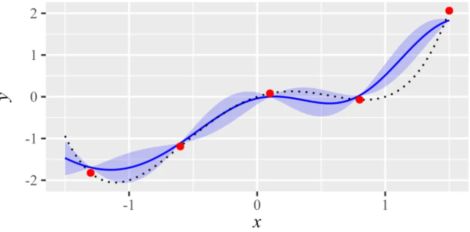
Example 2.3.2. As an extension of Example 2.3.1, Fig. 2.5 shows a model with a nugget of η = 0.1 but without re-interpolation. Figure 2.6 shows the same model with re-interpolation. In both cases, the nugget leads to a model that does not exactly reproduce all training samples.

-2 -1 0 1 2

-1 0 1

x

y

Figure 2.5:

The prediction

y(x)ˆ

of a Kriging model with nugget effect but without re-

interpolation (blue solid line) based on five data samples (red dots) from the true function

f(x) =x⁴−2x²+x

(black dotted line). The shaded region indicates the uncertainty estimate

of the model, i.e.,

y(x)ˆ ±s(x).ˆ

(27)

-2 -1 0 1 2

-1 0 1

x

y

Figure 2.6:

The prediction

y(x)ˆ

of a Kriging model with nugget effect and re-interpolation (blue solid line) based on five data samples (red dots) from the true function

f(x) = x⁴ − 2x²+x

(black dotted line). The shaded region indicates the uncertainty estimate of the model, i.e.,

y(x)ˆ ±s(x).ˆ

2.4 Efficient Global Optimization

The Efficient Global Optimization (EGO) algorithm’s [140] most distinctive feature is its use of the uncertainty estimate s ˆ

²

(x). EGO essentially follows the typical SMBO concept presented in Algorithm 3. The most important distinction occurs in Line 10.

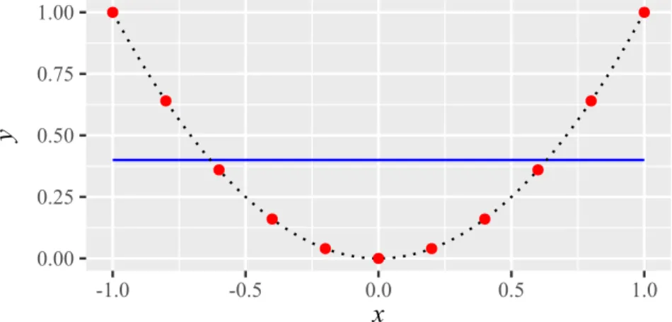
Here, EGO does not simply minimize the prediction, but rather optimizes a so-called infill criterion. In EGO, this infill criterion is the Expected Improvement (EI) [175, 140]. Other infill criteria include, e.g., the Probability of Improvement (PI) or the Lower Confidence Bound (LCB) [93].

For each sample x, the Kriging model specifies a normal distribution with mean y(x) ˆ and variance s ˆ

²

(x). Based on that distribution, we can estimate a probability of reach- ing a certain objective function value or better. For the model from Example 2.3.1, Fig. 2.7 shows the corresponding probabilities. The PI of each sample x is the de- picted probability along the dashed line that marks the best-observed function value.

Unfortunately, the PI does not consider how large a potential improvement is. Here, the improvement implies the difference between a potential function value and the best- observed value. Clearly, improvements cannot be negative. Hence, the improvement is defined as

I(ˆ y) = max

min(y) − y ˆ , 0

.

If the PI is large, but the improvement itself is extremely small, the corresponding

sample may not be a very promising candidate solution. The EI intends to alleviate

this. It is the expectation of I (x). In contrast to the PI, it takes the likelihood as well

as the magnitude of the improvement into account.

(28)

28 2.4. EFFICIENT GLOBAL OPTIMIZATION

-2 -1 0 1 2

-1 0 1

x

y

0.2 0.4 0.6 0.8

probability

Figure 2.7:

The prediction of a Kriging model without nugget (blue solid line) based on five data samples (red dots) from the true function

f(x) =x⁴−2x²+x

(black dotted line). The color scale of the background presents the probability of attaining the corresponding

y

value or better. The dashed black line marks the best-observed function value. Improvements only occur below that line.

The EI of a sample x is [140]

EI(x) = (

y

^∗

Φ

y^∗ ˆ s(x)

+ ˆ s(x)φ

y^∗ ˆ s(x)

if s ˆ (x) >0

0 else , (2.6)

The EI is based on y

^∗

= min(y)−ˆ y(x), the cumulative distribution function Φ(.) of the normal distribution, and the probability density function φ(.) of the normal distribu- tion. Furthermore, min(y) returns the minimum of all observed function values y. In each iteration of the EGO algorithm, the EI(x) is maximized. The resulting candidate solution x is evaluated with the expensive objective function f(x).

EI is very useful to balance the trade-off between exploitation and exploration in SMBO. By respecting both the prediction y(x) ˆ and the uncertainty estimate s(x), EI ˆ drives the search into poorly explored regions with potentially good function values.

It may prevent cases where a Kriging-based optimization algorithm would get stuck in local optima. Once a local optimum has been found, the EI of nearby solutions is close to zero (and exactly zero at the local optimum itself). Here, we understand a local optimum as a candidate solution with neighbors of equal or worse fitness.

Note that algorithms like EGO are also known as Bayesian optimization, following the

terminology of Mockus et al. [175].

(29)

Chapter 3 A Survey of Surrogate Models for Discrete Problems

Chapter 2 described basic SMBO approaches established for real, vector-valued search spaces, with x ∈ X ⊆ R

^m

. This chapter comes back to the focus of this thesis: the broad class of search spaces, x ∈ X where X is some nonempty set, e.g., representing discrete, combinatorial, or mixed search spaces.

As already mentioned in Section 1.1, SMBO approaches were rarely discussed in the context of combinatorial, discrete, or mixed optimization. This scarcity is unlikely due to a lack of problems in this field. Rather, suitable surrogate modeling methods are not available or known to experts in potential application domains. To close this gap and to provide a background for our contributions, we provide a survey of discrete surrogate modeling techniques.

3.1 Strategies for Dealing with Discrete Structures

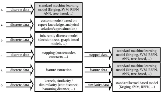
For surrogate modeling in discrete search spaces, six strategies (STR) can be identified in the literature.

STR-1 The naive approach: As long as the data can still be represented as a vector (bi- nary variables, integers, categorical data, permutations) the discrete structure can be ignored. SMBO can be applied without any modifications.

All following sections of this chapter are based on parts of the article“Model-based Methods for Continuous and Discrete Global Optimization”by Bartz-Beielstein and Zaefferer [26].

This includes many text elements that are taken verbatim from that publication. In the article, the discussion of continuous optimization methods was mostly contributed by Thomas Bartz- Beielstein. The part that is relevant to this chapter was mostly contributed by the author of this thesis. The survey was rewritten, restructured, and expanded. To a lesser extent, a few considerations have been taken from the article“Efficient Global Optimization for Combinatorial Problems”by Zaefferer et al. [273].

(30)

30 3.2. NAIVE APPROACH

mapped data

feature data

similarity data standard machine learning

model (Kriging, SVM, RBFN, ANN, tree-based, ...) discrete data

custom model (based on expert knowledge, analytical

solution/approximation) discrete data

1.

inherently discrete model (decision trees, graph-based

models, ...) discrete data

mapping (autoencoder, contrasts, ...) discrete data

feature extraction discrete data

kernels, similarity / dissimilarity (edit distance,

hamming distance, ...) discrete data

2.

3.

4.

5.

6.

standard machine learning model (Kriging, SVM, RBFN,

ANN, tree-based, ...) standard machine learning model (Kriging, SVM, RBFN,

ANN, tree-based, ...) standard kernel-based model

(Kriging, SVM, RBFN, ...)

Figure 3.1:

Six different strategies for surrogate modeling in discrete search spaces.

STR-2 Customized models: A specific modeling solution is tailored to fit the needs of a certain application.

STR-3 Inherently discrete models: Some models already are discrete by their own design.

STR-4 Mapping: Discrete variables or structures are mapped to a more easily treatable representation.

STR-5 Feature extraction: Instead of directly modeling the relation between an object (or its representation) and its quality, it is possible to calculate numeric fea- tures of the object. The resulting feature values can be modeled with standard techniques.

STR-6 Kernel-based modeling: Where available, discrete kernels (measures of (dis)- similarity) may be used to replace continuous kernels that, e.g., are employed in models like k-Nearest Neighbors (k-NN) [39], SVM [224], RBFN [39], or Kriging.

The subsequent sections present key characteristics of the strategies, and summarize the relevant literature.

3.2 Naive Approach

The most basic strategy to deal with a discrete search space X is to simply ignore the

nature of the search space and apply the usual methods from continuous optimization.

(31)

Clearly, this is only feasible if the sample x ∈ X can still be represented as a vector.

Especially if the discrete variables are of an ordinal nature, the naive approach may still be successful. A potential drawback of this approach is that the model’s input space may have large areas of redundancy. Or else, this approach may create large areas of infeasible solutions. Depending on the employed optimization algorithm, this may deteriorate performance compared to strategies that are more advanced.

3.3 Customized Models

A more sophisticated approach is to employ customized, application specific solutions.

On the one hand, this procedure can be very efficient because it integrates significant prior knowledge into the model. On the other hand, a customization approach may in- troduce bias. The result may be hard to transfer to other applications or data structures.

If applicable at all, customized models often require significant effort or knowledge of the application domain expert. Clearly, this approach is not applicable to true black- box problems.

One example for customized models is presented by Voutchkov et al. [254]. They optimize a weld sequence, which is represented as a signed permutation. Here, the weld path is divided into segments. The permutation specifies the order in which those segments are welded. Each sign indicates the direction in which a segment is welded. They attempt to find a weld sequence that yields a minimal displacement due to thermal stresses. Simulating the displacement via a finite element model is com- putationally expensive. Hence, Voutchkov et al. suggest replacing it with a surrogate model by estimating the influence of each segment in the weld sequence, based on previously simulated weld sequences. In addition to the objective function values, this surrogate model also exploits intermediate results that can express the impact of in- dividual segments, depending on their position in the weld sequence. Voutchkov et al. [254] find a near-optimal welding sequence by evaluating only 28 out of 46, 080 possible sequences. Variations of this approach for weld sequence optimization are described by Asadi and Goldak [11], and Bonnaud [42]

For binary problems, Verel et al. [252] suggest a model based on the Walsh decompo- sition. In terms of model quality, they show that the Walsh model tends to outperform Kriging on larger data sets. We categorize the Walsh model as a customized model because it cannot be immediately transferred to other problem classes, such as per- mutation problems. Still, similar decomposition approaches may be devised for other problem classes.

Another example is presented by Nguyen et al. [192], who use a simplified objective

function (a simulation model for job shop scheduling) as a surrogate model in genetic

programming. They actively attempt to reduce the complexity of the objective func-

tion (e.g., reduced simulation times, reduced number of machines or operations). This

approach is also used by Mei et al. [174]. Similarly to the weld sequence optimization

approach, a simplification of the simulation model is specific to the considered applica-

tion. While similar simplifications may be possible with most simulation optimization

(32)

32 3.4. INHERENTLY DISCRETE MODELS

problems, it is infeasible to apply this approach to a problem that is not based on a simulation procedure.

Following these examples, many classical approaches in combinatorial optimization could also be labeled as customized surrogate models. Consider for instance the trav- eling salesperson problem. Here, to optimize the cost of visiting a set of locations, a permutation is optimized such that the traveled distance is minimal. Clearly, this model is only an approximation of reality. It does not account for many aspects of the real-world problem, e.g., stochasticity of actual travel costs or asymmetric travel costs between locations. Hence, the TSP model could be understood as a (customized) surrogate model. In this sense, customized surrogate models could be thought of as a standard approach towards solving combinatorial optimization problems.

3.4 Inherently Discrete Models

Some models are themselves discrete. One example is the class of tree-based models, such as regression trees or random forests. Random Forests have already been em- ployed as surrogate models in the field of algorithm tuning [126, 128, 246, 80, 125, 38, 198, 72].

On the one hand, these models easily deal with discrete data. They are an intuitive way to incorporate binary, categorical, or ordinal integer variables.

On the other hand, this strategy may fail if the discrete structures become more com- plex (e.g., graphs). Furthermore, in a mixed-variable case, a tree-based model is not ideal to represent the continuous parameters in the mix. This issue may require the coupling of a discrete model and a continuous one, e.g., treed Gaussian pro- cesses [106, 107]. Finally, discrete models may not always provide features required by the optimization algorithm. For example, uncertainty estimates can be derived from random forests by estimating the variance from the prediction of all trees in the for- est. Unfortunately, such an estimate does not have the same useful properties of the uncertainty estimates of a Kriging model (cf. Section 2.3.3).

3.5 Mapping

Another important approach to discrete surrogate modeling is to map from the com- plex, discrete space to another space that is easier to handle. Frequently employed approaches are dummy variables and contrasts. They are often applied in the context of classical linear regression models. A categorical variable can be mapped to a set of dummy variables, where each dummy represents a single level of the original variable.

This is the same as the one-hot encoding, i.e., only one of several bits can be 1. The n

_cat

levels of the categorical variable are mapped to n

_cat

binary variables. The resulting bi- nary variables are still discrete, but can be handled by standard regression approaches.

Alternatively, a map to (n

_cat

Surrogate models for discrete optimization problems

O PTIMIZATION P ROBLEMS

Dissertation

zur Erlangung des Grades eines

D OKTORS DER I NGENIEURWISSENSCHAFTEN

der Technischen Universität Dortmund an der Fakultät für Informatik

von

M ARTIN Z AEFFERER

Dortmund

2018

Tag der mündlichen Prüfung:

19. Dezember 2018 Dekan:

Prof. Dr.-Ing. Gernot A. Fink Gutachter:

Prof. Dr. Günter Rudolph, Technische Universität Dortmund

Prof. Dr. Thomas Bartz-Beielstein, Technische Hochschule Köln

This thesis was some years in the making. During these years, it profited from the indispensable support (moral and professional) of many people. Hence, I express my gratitude to my

• supervisor Prof. Dr. Thomas Bartz-Beielstein, who triggered my interest into this research field. He has since been a strong support and a source of motivation for my scientific work.

• supervisor Prof. Dr. Günter Rudolph. Our discussions always provided new impulses, and opened up questions that I might not have touched on otherwise.

• mentor Prof. Dr. Gabriele Kern-Isberner, for helpful discussions on work-life- balance, ideation, and systematic approaches of research.

• parents Monika and Rolf Zaefferer, for the patient support and encouragement

during these years.

4 CONTENTS

Contents

1 Introduction 9

1.1 Incentive . . . . 9

1.2 Objective . . . . 10

1.3 Synopsis . . . . 11

1.4 Publications . . . . 12

I Background and State of the Art 15 2 Continuous Methods for Expensive Black-box Optimization 16 2.1 Evolutionary Algorithms . . . . 16

2.2 Surrogate Model-based Optimization . . . . 20

2.3 Introduction to Kriging . . . . 22

2.3.1 Kriging Model . . . . 22

2.3.2 Kriging Prediction . . . . 24

2.3.3 Uncertainty Estimate . . . . 24

2.3.4 Nugget Effect . . . . 25

2.4 Efficient Global Optimization . . . . 27

3 A Survey of Surrogate Models for Discrete Problems 29 3.1 Strategies for Dealing with Discrete Structures . . . . 29

3.2 Naive Approach . . . . 30

3.3 Customized Models . . . . 31

3.4 Inherently Discrete Models . . . . 32

3.5 Mapping . . . . 32

3.6 Feature Extraction . . . . 34

3.7 Kernel-based Models . . . . 34

3.8 Alternative Models . . . . 36

3.9 Conclusions . . . . 37

4 Kernels: Terminology and Definitions 38 4.1 Motivation: The Kernel Trick . . . . 38

4.2 Similarity Measures . . . . 41

4.3 Dissimilarity Measures . . . . 41

4.4 Definiteness . . . . 43

4.4.1 Definiteness of Matrices . . . . 43

4.4.2 Definiteness of Kernels . . . . 44

4.5 Conditioning of Matrices . . . . 45

II Main Contributions 46 5 Kriging-based Combinatorial Optimization 47 5.1 Kriging for Combinatorial Data . . . . 47

5.2 Combinatorial Efficient Global Optimization . . . . 49

5.3 Proof of Concept . . . . 51

5.3.1 Case Study: Kriging with Hamming Distance . . . . 51

5.3.2 Results and Analysis . . . . 55

5.3.3 Case Study: Changing the Distance Function . . . . 58

5.4 Conclusions . . . . 59

6 How to Find the Right Kernel 61 6.1 Selecting Kernels . . . . 63

6.1.1 Random Selection . . . . 63

6.1.2 Selection with Correlation Measures . . . . 64

6.1.3 Selection with Maximum Likelihood Estimation . . . . 65

6.1.4 Selection with Cross-Validation . . . . 66

6.2 Combining Kernels . . . . 66

6.2.1 Weighted Sum via Linear Regression . . . . 67

6.2.2 Weighted Sum via MLE . . . . 68

6.2.3 Weighted Sum via Stacking . . . . 69

6.2.4 Superposition of Kriging Models . . . . 71

6.3 Experimental Validation . . . . 72

6.3.1 Experimental Setup . . . . 72

6.3.2 Results and Discussion . . . . 73

6.4 Conclusions . . . . 80

7 Definiteness of Distance-based Kernels: An Empirical Approach 82 7.1 Dealing with Definiteness . . . . 83

7.2 Probing Definiteness . . . . 83

7.2.1 Random Sampling for Probing Definiteness . . . . 84

7.2.2 Optimization for Probing Definiteness . . . . 85

7.3 Experimental Validation . . . . 86

7.3.1 Random Sampling . . . . 86

7.3.2 Optimization . . . . 86