Patterns of genetic recombination and variation in the human genome

Patterns of genetic recombination and variation in the human genome

Inaugural – Dissertation zur

Erlangung des Doktorgrades

der Mathematisch- Naturwissenschaftlichen Fakultät der Universität zu Köln

Vorgelegt von Ekaterina Shabanova aus Astrachan, Russland

Köln 2009

Berichterstatter: Prof. Dr. Thomas Wiehe

Prof. Dr. Jonathan Howard

Tag der muendlichen Pruefung: 20 October 2009

Abstract

Genetic recombination plays an important role in shaping genome variation. It enhances haplotype diversity, helps to maintain genome integrity and ensures the proper segregation of the chromosomes. While participating in DNA rearrangement, recombination is not an “independent player”. It is tightly connected and influenced by other genomic features, such as nucleotide diversity. A correlation between nucleotide diversity and recombination rate was observed in the human genome, as well as in the genomes of other organisms (Arabidopsis, Drosophila, etc). The traditional view that selection has contributed to shape this pattern was questioned by the view that it may solely be due to a mutagenic effect. Extensive analysis of the data from dbSNP and broad scale recombination maps revealed a high degree of uncertainty in the inferred correlation coefficients. One goal of this study was to re-assess the magnitude and disentangle the possible reasons for this observation. The results show that there is no evidence for a presence of strong correlation between nucleotide diversity and recombination rate. In fact, the observed effect can be due to insufficient data or poor data quality in earlier studies. Analysis of the more recent data shows that the correlation between diversity and recombination may be due to sequence composition, such as sequence composition. While looking at the fine scale it became clear that recombination hotspots are very ephemeral structures, which do not have influence on long-term molecular evolution. Only detailed experimental studies can reveal, whether the apparent correlation between diversity and recombination rate has a causal connection.

In order to obtain high resolution recombination rates, a single sperm typing approach was

applied to 2.5 Mb sequence consisting of four Encode regions on human chromosome 11. The

regions were selected not on the basis of classical linkage studies, but in unbiased fashion. The

outcome revealed a cross over rate of 0.12 cM/Mb, which was much lower compared to the

expected 1.875 cM/Mb according to high resolution recombination maps. We confirm an

increased gene conversion rate compared to cross over. Out of 10 recombinants, 7 had conversion

haplotypes. We assume that such a low cross over rate can be due to the individual or sex-

specific variation. Our data did not support genetic characteristics known to be associated with

gene conversion or recombination in general. For instance, identified conversion tracts did not

have a high GC content. No association between converted or cross over regions and a 13-mer

degenerate motif (predicted to be associated with recombination hotspots) was observed. The

observed CpG fraction was so low compared to the expected, that the possible explanation could be a extensive methylation of the converted regions. Finally, we hypothesize, that there is a difference in regulation mechanism as well as in frequency of double-strand breaks resolved as conversion events in short and long tract conversions. The frequency of the breaks can also be a reason to differentiate hotspots-associated conversions and the ones occurring in coding regions.

Kurzzusammenfassung

Genetische Rekombination spielt eine tragende Rolle in der Gestaltung der Genom-Variation. Sie fördert die Haplotyp-Diversität, unterstützt die Aufrechterhaltung der Genom-Integrität und stellt eine korrekte Segregation der Chromosomen sicher. Trotz ihrer tragenden Rolle in der Reorganisation von DNA-Sequenzen, ist Rekombination keine unabhängige evolutionäre Kraft.

Sie steht im Wechselspiel mit anderen genomischen Merkmalen, und wird zum Beispiel von der Nukleotid-Diversität beeinflusst. Die Korrelation zwischen Nukleotid-Diversität und Rekombinationsrate wurde in den letzten Jahren im menschlichen Genom, aber auch in den Genomen anderer Spezies, wie zum Beispiel Arabidopsis oder Drosophila, beobachtet. Die traditionelle Sichtweise, dass natürliche Selektion diese Korrelation mitbeinflusst hat, wird durch die Ansicht, dass dies alleinig auf den „mutagenischen Effekt“ zurückzuführen sei, in Frage gestellt. Eine umfangreiche Analyse von dbSNP-Daten und grob-skalierte Rekombinationskarten offenbarten eine grosse Unsicherheit in der Richtigkeit der gewonnenen Korrelationskoeffizienten. Ein Ziel dieser Arbeit war es, die Stärke der Korrelation neu abzuschätzen und mögliche Gründe für diese Beobachtung aufzudecken. Die Resultate der Studie konnten keine starke Korrelation nachweisen. Der beobachtete Effekt kann durch unzureichende Daten oder die niedrige Datenqualität in früheren Studien erklärt werden. Die Analyse neuerer Datensätze zeigt, dass die Korrelation zwischen Diversität und Rekombination eventuell auf die DNA-Sequenz-Zusammensetzung zurückzuführen ist. In Fein-Skala Untersuchungen zeigte sich außerdem, dass Rekombinationshotspots sehr kurzlebige Erscheinungen sind, und deshalb keinen Einfluss auf die langfristige molekulare Evolution haben. Nur durch detaillierte experimentelle Studien kann diese Korrelationsfrage besser ergründet werden.

Um Rekombinationsraten in einer hohen Auflösung zu bestimmen wurde der Spermien-

Typisierungs-Ansatz auf Sequenzen einer Gesamtlänge von 2.5Mb bestehend aus vier Encode-

Regionen des menschlichen Chromosoms 11 angewendet. Die Regionen wurden zufällig

ausgewählt ohne auf klassische Linkagestudien zurückzugreifen. Als Ergebnis zeigt sich eine

Crossing-Over-Rate von 0.12 cM/Mb, die im Vergleich zu den erwarteten 1.875 cM/Mb sehr

niedrig ist. Es konnte eine im Vergleich zur Cross-Over Rate erhöhte Genkonversionsrate

bestätigt werden. Von zehn Rekombinanten weisen sieben Konversionshaplotypen auf. Die im

Ganzen niedrige Crossing-Over-Rate ist möglicherweise auf individuelle oder sex-spezifische

Variation zurückzuführen. Unsere Daten konnten genetische Merkmale, die im Allgemeinen mit Genkonversion oder Rekombination assoziiert werden, nicht bestätigen; zum Beispiel zeigten die identifizierten Genkonversions-Regionen keinen hohen GC-Anteil auf. Zudem konnte keine Assoziation zwischen Genkonversions- beziehungsweise Rekombinations-Regionen mit einem degenerierten 13-mer-Motiv, dass für Rekombinationshotspots vorhergesagt wurde, bestätigt werden. Der beobachtete CpG-Anteil war im Vergleich zur Erwartung so gering, dass die Möglichkeit einer beträchtlichen Methylation der konvertierten Regionen in Frage kommt. Zum Abschluss stellen wir die Hypothese auf, dass es einen Unterschied in den Regulationsmechanismen und in der Häufigkeit der Doppelstrangbrüche gibt, der sich als Konversions-Ereigniss in kurzen und langen Konversionen widerspiegelt. Die Frequenz der Doppelstrangbrüche kann eine Möglichkeit darstellen, hotspot-assoziierte Konversionen von jenen in kodierenden Regionen zu unterscheiden.

Table of Contents

Abstract……….…1

Kurzzusammenfassung……….3

Table of Contents………..…5

1. Introduction………8

1.1 Processes influencing variation of the human genome………..8

1.2 Genetic recombination, forms and definition………...9

1.3 Cross over………...9

1.4 Importance of meiotic recombination………...10

1.5 Mechanism of the homologous recombination……….……10

1.6 Recombination rate variation and hotspots………...13

1.7 Hotspot detection………..13

1.7.1 Linkage maps based on pedigree data………...14

1.7.2 Linkage Disequilibrium in recombination mapping………...14

1.7.3 Sperm typing analyses………...15

1.8 Hotspots evolution………....15

1.9 Meiotic gene conversion………...…16

1.10 Association of recombination with other genomic features……….…..16

1.11 Technological limitations and future perspectives of the recombination analysis……….……..18

1.2 The aims of the study………...18

1.3 Experimental regions of interest……….……..19

2. Materials and Methods………20

2.1 Material (sperm collection)………..20

2.2 Experimental methods……….….20

2.3 Theoretical methods……….…30

3. Results……….…...31

3.1 Recombination and variability in public data……….………..31

3.2 Specificity of sperm sorting on FACSVantage SE Cell Sorter………38

3.3 Estimation of the cross over rate………..40

3.4 Annotation of the ENCODE regions……….…...42

3.4.1 Chromosome 11 at a glance……….…..42

3.4.2 ENm009………....45

3.4.3 ENr332………..………….47

3.4.4 ENm003………...48

3.4.5 ENr312………..….51

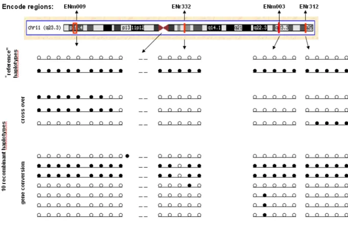
3.5 Haplotype screen……….….52

3.5 .1 “Reference” haplotypes……….…...54

3.5.2 Recombinant haplotypes………...54

3.5.3 Cross over and gene conversion events within and near ENm 009………...55

3.5.4 Conversion events in ENmr332……….…60

3.5.5 Conversion tracts in ENm003………....65

3.5.6 Cross over ENr312………67

4. Discussion……….….70

4.1 Analysis of correlation between SNP density and recombination rate in the human genome………...70

4.2 Analysis of experimental cross over data………71

4.3 Analysis of gene conversion events……….73

Summary of the results………77

Implication of the study………...78

Outlook……….….78

Reference List……….…79

Appendix………86

Acknowledgements………96

1. Introduction

1.1 Processes influencing variation of the human genome

Genetic variability, in a way, measures how much the trait or the genotype will tend to vary in a population (Burt, 2000). The presence of variability in a population is an important factor in a number of fundamental biological processes, such as shaping biodiversity, evolutionary development of a population and susceptibility to diseases (Wills and Christopher, 1980). The role of variability for biodiversity can be seen in successful adaptation to environmental conditions and, thus, contributes to success in avoiding extinction. Variability also plays a crucial role in evolution: it stimulates individual responses to environmental stresses and can lead to survival of the fittest variants because of natural selection. Genetic variability has become one of the factors contributing to an increased interest in “personalized medicine” since it underlies differential susceptibility to diseases and sensitivity to toxins or drugs (Burt, 2000).

There are a few known sources of genetic variability in a population. One of them is genetic recombination. Recombination is also variable in frequency and location and thus, it can be selected for to increase fitness, because more recombination leads to more variability; this increased genetic variability makes it easier for a particular population to handle changes (Burt, 2000). Genetic mutations are the main source of genetic variability within a population.

Mutations can have positive, negative or neutral effects on fitness (Wills and Christopher, 1980).

Natural selection can propagate mutation-induced variability through the population if the mutation is beneficial or its effect will be hidden if the mutation is deleterious. The excess of deleterious mutations is typically observed in smaller populations with reduced variability levels (Wills and Christopher, 1980).

Other sources contributing directly or indirectly to genetic variability include immigration,

emigration and translocation. When an individual moves in or out of a population, genetic

variability in the next generation will increase if it reproduces (Linhart et al. 2003). Polyploidy in

sexual organisms provides yet another source; it allows more recombination during meiosis and,

therefore, leads to more genetic variability in the offspring.

In asexual organisms with limited sources of variability, diffused centromeres can become one, since they allow the chromatids to split apart in variety of ways and assists chromosome fragmentation and polyploidy to create more variability (Linhart et al. 2003).

In this study, specific attention will be given to genetic recombination as a source of genetic variability.

1.2 Genetic recombination, forms and definition

Genetic recombination is the transmission-genetic process by which chromosomes are broken and then rejoined to form a new genetic combination, different from the original (Brooker, 1999).

A major type of genetic recombination is homologous recombination, which is an essential feature of all sexual organisms. It occurs between DNA segments homologous to each other. This process enhances genetic diversity, helps to maintain genome integrity (when genome is capable of multiplication, variation and heredity) and ensures the proper segregation of chromosomes.

Another type is site-specific recombination, where non-homologous segments are recombined at the specific sites. This type of recombination happens within genes that encode antibody polypeptides and also occurs when certain viruses integrate their genomes into host cell DNA.

The third type of recombination is known as transposition. Small segments of DNA called transposons can move themselves to multiple locations within the host’s chromosomal DNA (Brooker, 1999).

It should be noted that a number of other genetic exchanges do not fall into any of the above classes, and are named illegitimate recombination or recombination without homology (Brooker, 1999).

1.3 Cross over

Chromosomal crossover (or crossing over) is the exchange of genetic material between

homologous chromosomes during prophase I of meiosis, in a process called synapsis. Synapsis

begins before the synaptonemal complex develops, and is not completed until near the end of

prophase I. Crossover usually occurs when matching regions on matching chromosomes break

and then reconnect to the other chromosome. The result of this process is an exchange of genes,

called genetic recombination. Chromosomal crossovers also occur in asexual organisms and in

somatic cells, since they are important in some forms of DNA repair (Li and Heyer, 2008).

1.4 Importance of meiotic recombination

In most eukaryotes, a cell carries two copies of each gene, each referred to as an allele. Each parent passes on one allele to each offspring. An individual gamete inherits a complete haploid complement of alleles on chromosomes that are independently selected from each pair of chromatids lined up on the metaphase plate. Without recombination, all alleles for those genes linked together on the same chromosome would be inherited together. Meiotic recombination allows a more independent selection between the two alleles that occupy the positions of single genes, as recombination shuffles the allele content between homologous chromosomes (Brooker, 1999).

Meiotic recombination is one of the fundamental biological mechanisms leading to exchange of genetic material between homologous chromosomes. During meiosis, this process is also associated with a few important cellular functions such as the formation of the synaptonemal complex and proper chromosome segregation (Padhukasahasram et al. 2006). The role of meiotic recombination in evolutionary biology is to produce novel allelic combinations to increase genetic diversity within a population.

To understand the variation of the recombination rate is one of the goals in association mapping and evolutionary inference studies in particular, and in molecular biology in general.

(Padhukasahasram et al. 2006).

1.5 Mechanism of the homologous recombination

The most famous central model of the molecular steps occurring during homologous recombination was proposed by R. Holliday in 1964. It is based on studies of Ustilago maydis (a simple eukaryote) and explains both cross over and gene conversion events (Brooker, 1999).

At the beginning of the process (Fig.1) two homologous chromosomes are aligned with each

other. During the first step a break occurs at the identical sites in one strand of both parental

chromosomes. During the second step the strands invade the opposite helices and base pair with

the complementary strands. In the third step this event is followed by the covalent linkage of

DNA to create a Holliday junction (a structure, which incorporates four strands of DNA, two of each homologous chromosomes).

As shown in step six (Fig.1), the cross in the Holliday junction can migrate in a lateral direction.

As it does so, a DNA strand in one helix is being swapped for the DNA strand in the other helix.

This process is called branch migration, because the branch connecting the two double helices migrates laterally. Since the DNA sequences in the homologous chromosomes are similar but not identical, the swapping of the DNA strands during branch migration may produce regions in the double stranded DNA called heteroduplexes. A heteroduplex is a DNA double helix that contains mismatches. Their occurrence is explained by the fact that the DNA strands come from homologous chromosomes and their sequence is not perfectly complementary.

The next step (step 7 in Fig.1) is isomerization, during which the Holliday structure may make an 180º turn. The two structures existing in this step are structural isomers of each other (chemically identical except for the location of certain segments). The final steps of the recombination processes are called resolution, since they involve the breakage and rejoining of two DNA strands to create separate chromosomes. In other words, the entangled DNA strands become resolved into two separate structures. Resolution can occur in two ways (step 8, Fig.1). The first way is without isomerization (8b, Fig.1). The breakage could occur at the same strands that were broken in the first step. In this case at the resolution, the strands are rejoined to produce a non- recombinant pair of chromosomes. The second way is with isomerization, and then the resolution phase can involve breakage of the two DNA strands that were not broken before in the first step.

In this case, the rejoining of the corresponding strands produces two recombinant chromosomes

(step 8a, Fig.1). The original Holliday model was based on the results of observed cross over

events in fungi where the products of meiosis are contained in the same single ascus (the sexual

spore-bearing cell produced in ascomycete fungi). Nevertheless, molecular research in many

other organisms has supported the central tenets of the Holliday model (Brooker, 1999).

Fig.1. The Holliday model for the homologous recombination from Brooker RJ(1999); 8a -

the resolution of the Holliday complex into cross over product; 8b – the resolution of the

Holliday complex into a non-recombinant heteroduplex.

1.6 Recombination rate variation and hotspots

The rate of meiotic recombination (i.e., crossing over) in humans varies on different physical scales (Lynn et al. 2004). While the broad-scale rates are relatively similar across populations and possibly across species (Serre et al. 2005, Ptak et al. 2005), on the fine scale, the situation is different: most cross over events tend to be concentrated into 1-2 kb regions named

“recombination hotspots”. In addition to this, “cold spots” or regions of low recombination rate have also been noted (Petes 2001). Crossover initiation sites can be distributed randomly throughout the genome, but the rate of initiation at particular sites can be significantly higher at some genomic regions compared to others (Arnheim et al. 2003).

There is much evidence that shows variation of hotspots within a population through time (Jeffreys et al. 2005), as well as a lack of hotspot conservation between human and chimpanzees (Wall et al. 2005, Ptak et al. 2005). There are a few reasons why it is important to understand the mechanistic underpinning of hotspots (Petes 2001). One such reason is to understand the recombination initiating mechanism, which requires knowledge of factors regulating both hotspots and cold spots. Other reasons include: the number of recombination events per chromosome is relevant to the accuracy of chromosome segregation; distribution of exchanges influences the probability of assembling new configurations of physically linked genes during evolution and, finally, understanding hotspots and cold spots will assist in understanding other DNA-related processes affected by chromosome context, e.g., transcription and replication (Petes 2001).

1.7 Hotspot detection

There are a few approaches developed to infer recombination rates and map genomic hotspots.

Two approaches have gained particular popularity: estimates can be obtained either indirectly

through examining patterns of marker association (linkage disequilibrium), established through

population dynamic processes, or directly through labor-intensive screening of millions of sperm

for recombinant DNA molecules within relatively short genomic intervals (Webb et al. 2008).

1.7.1 Linkage maps based on pedigree data

Constructing a linkage map is one of the common approaches to obtain recombination rates. The cross over events are inferred from the transmission patterns of polymorphic markers in a large pedigree or in extensive crosses (Coop and Przeworski, 2007). The rates of genetic exchange between markers are converted into a linkage map by use of a function that takes into account a model of cross over interference. To obtain the cross over rates, it is necessary to compare the genetic map with the physical one. This approach is widely used to characterize variation among individuals, but, since it relies on estimates of recombination from transmitted chromosomes, this method misses half of the cross over events that occur in meiosis or those any gametes that are selected against (Coop and Przeworski, 2007).

1.7.2 Linkage Disequilibrium in recombination mapping

This approache utilizes a population genetic model to relate the patterns found in a current polymorphism sample to the historical rate of recombination (McVean et al. 2004). The estimates of historic rates encompass thousands of meioses of the sample’s history, so the rate is estimated as an average of male and female rates over time (Coop 2005).

Recent studies identified considerable variation of linkage disequilibrium across the human genome (Gabriel et al. 2002; Phillips et al. 2003, Arnheim et al. 2003), which reflects variation in the underlying recombination rate (Reich et al. 2002; Wang et al. 2002a and b; Innan et al. 2003;

Phillips et al. 2003). There is a certain correlation between uneven recombination rate distribution and existence of LD blocks in certain genomic areas, although not all LD blocks can be explained by recombination variation (Arnheim et al. 2003). Recombination maps available by 2002-2003 were very inaccurate for intervals smaller than 1 cM (Kong et al. 2002; Weber 2002). This inaccuracy complicated revealing to what extent LD variation is determined by variation in recombination. Recently, the International HapMap project has mapped the LD landscape on a kilobase level fo the entire genome. The data allowed detection of the global recombination landscape at high resolution by using coalescent analyses and observed haplotypes were explained through in silico reconstruction with variable recombination rates (Webb et al. 2008).

These studies revealed approximately 33 thousand putative cross over hotspots, their distribution

and population-specific activity, as well as provided data on motifs possibly associated with them

(Altshuler et.al., 2005).

1.7.3 Sperm typing analyses

A sperm-typing approach allows direct observation of cross over events in male individuals and produces a uniquely detailed picture of the current recombination rate at a finer-scale (Coop 2005). Sperm typing enabled for the first time to measure human recombination fractions in a single individual (male), because the large number of sperm available from a single donor permits a high level of accuracy to be achieved (Arnheim et al. 2003). In contrast to LD hotspot mapping, few human recombination hotspots have been directly characterized in sperm and the obtained data does not completely explain whether linkage disequilibrium data predicts genuine hotspots accurately, or correctly determines their historical activity (Webb et al. 2008). Due to Webb et al data (2008) up to date sperm typing covered approximately 0.6 Mb of the human genome. One major goal was the identification of hotspots with special focus on the MHC region, where approximately seven hotspots were characterized (Jeffreys et al. 2000, Jeffreys and Neumann 2002, Kauppi et al. 2005). In contrast, the entire chromosome 1 contains only eight hotspots (Jeffreys et al. 2000, Jeffreys et al. 2005). These studies revealed additional phenomena such as variation in hotspot activity between different male individuals, as well as polymorphic sites driving activity of the hotspot (Neumann, Jeffreys 2006). In most cases, hotspots obtained by sperm typing and linkage disequilibrium hotspots are in good concordance (Webb et al. 2008).

1.8 Hotspots evolution

The availability of high-resolution approaches mentioned above allowed the characterization of hotspots as ephemeral structures that are quick to evolve within a single population and even between individuals of the same population. There is experimental evidence for differences in recombination activity in the CAP10 genomic region between African ancestral and European and Asian populations (Clark et al. 2007). Sperm typing showed different intensities in the MSTM 1a hotspot in 26 male individuals (Neumann and Jeffreys 2006). The difference between female and male rates should also be noted (Coop and Przeworski, 2007). One of the possible explanations for a hotspot’s quick development could be the presence of a certain motif, polymorphic site or other “control element” (modifier) that can be associated with the hotspot.

The loss of such an element (e.g., during DNA repair) can potentially result in further decrease of

recombination activity within the region.

1.9 Meiotic gene conversion

Homologous gene conversion is considered as a poorly characterized form of recombination (Gay et al. 2007), a non-reciprocal process acting on short lengths of DNA, where genetic material from one parental chromosome is incorporated into an alternate chromosome during meiotic exchange (Szostak et al. 1983). Cross over events are believed to include gene conversion tracts as well, which can not be detected by current population-based methods.

Therefore, initially the term gene conversion defined events not accompanied by cross over (Gay et al. 2007). Gene conversion in the human genome is believed to be up to 15 times as frequent as cross overs (Jeffreys and May 2004). These events are difficult to track because of the short length of DNA transferred – with an average size of approximately 350 bp – which represents a difficulty in marker selection. When the close association between cross overs and gene conversion events was revealed, some of the characterized hotspots with higher polymorphism levels were investigated for conversion activity (Jeffreys and May 2004). The results revealed the more active the hotpot was the more conversion events were observed.

1.10 Association of recombination with other genomic features

The extent to which adaptive evolution shaped the recent evolutionary history in humans is much debated (Spencer et al. 2006). However, adaptive evolution is expected to leave its footprint in the patterns of genetic variation. In regions of high recombination, the footprint is expected to be smaller, since recombination moves a beneficial mutation onto different genetic backgrounds allowing linked diversity to occur. Therefore, the observed positive correlation between nucleotide diversity and recombination rate suggests that many loci were or still are the targets of adaptive evolution (Spencer et al. 2006).

In 1992, Aquadro and Begun explained the presence of a correlation between nucleotide diversity

and recombination rate in Drosophila by positive selection (hitchhiking) acting on certain regions

in the genome. In 1998, M. Nachman observed a correlation between diversity and recombination

at certain coding loci in humans. Selection (background or hitchhiking) was proposed as the

possible explanation for this phenomenon. In 2002, Lercher and Hurst noticed a correlation at the

genome-wide scale. They also observed a correlation between human-mouse divergence and

recombination rate. They revealed that the correlation holds not only for coding regions or

control elements, but across the entire genome. Thus, they assumed that increased diversity in the

regions of higher recombination can be due to higher mutation rates. Based on these data the neutral hypothesis was proposed stating that recombination can be mutagenic.

In 2003, the new human, as well as the chimpanzee data supported the neutral explanation (Hellmann et al, 2003). The correlation between nucleotide diversity and recombination rate was observed within the human population, as well as the correlation between human-chimpanzee (human-macaque) divergence and recombination rate. They showed that regions with less recombination have reduced divergence to chimpanzee and baboon; diversity levels within these regions are also lower. This observation suggested an association between recombination and mutation and supported the neutral explanation for the presence of the positive correlation.

In 2005, with the availability of diversity and recombination data from different human deep- sequencing projects (HapMap and Encode), the presence of the correlation between nucleotide diversity and recombination rates was confirmed on the broad (megabase) scale, but since recombination rates were known to change rapidly on the finer sclale, they became better predictors of diversity than divergence (Hellmann et al. 2005). Recombination, diversity and divergence were found to be correlated with such genomic features as GC and CpG content, as well as with gene expression and gene density. As a result of that study, 12 parameters were investigated and confirmed to be correlated with both diversity (divergence) and recombination rates. Association with these features appeared to be a better explanation, rather than mutagenicity of recombination.

In 2006, the association between genomic features was confirmed (Spencer et al. 2006).

Recombination was shown to influence genetic diversity at the hotspot level, since both diversity

and recombination were positively correlated with sequence composition. This fact was used to

explain the broad-scale association as well. However, the hotspots were confirmed to have no

influence on the substitution rate, since they are ephemeral on an evolutionary time scale and

have little influence on broader scale patterns of base composition and long-term molecular

evolution (Spencer et al. 2006).

1.11 Technological limitations and future perspectives of the recombination analysis

One of the most important and obvious limitations of sperm typing is sex specificity: sperm typing measures recombination only in males, whereas haplotypes in human populations are the products of recombination events happening in both sexes (Arnheim et al, 2003). Although making conclusions about haplotype formation based only on male autosomes is still accepted, it is necessary to keep in mind that recombination rate in females is, on average, higher (Arnheim et al, 2003; Ptak et al, 2005). Moreover, there is substantial sex-dependent regional genomic variation. Thus, in the mouse, one of the MHC hotspots was identified only in female individuals (Isobe et al, 2002). These types of data are not available in humans, because to date, it is not possible to isolate female gametes in sufficient amounts to conduct a high-resolution study at the same level as in sperm cells (Arnheim et al., 2003).

Another possible limitation is the formation of a new haplotype by gene conversion that can be cross over-associated or not (Arnheim et al, 2003). Technical limitations of the sperm-typing methods should be taken into account as well. The most important requirement is the presence of heterozygous polymorphic markers (at least two flanking the region of interest). As a condition for future recombination analysis, deeper sequencing and mapping of polymorphic markers to infer population and individual specific Linkage Disequilibrium patterns and, thus, recombination rates, is needed.

Also, most of the hotspots characterized experimentally are located within MHC, PAR-1, beta- globin and other highly recombining areas. All together, they belong to approximately 0.6 % of the genome. How representative these regions are remains unknown (Arnheim et al. 2003).

Clearly, high-resolution recombination analysis should be performed in an unbiased fashion on different chromosomal segments. Choosing regions based on classical linkage studies can be misleading since most of predicted hotspots may not be found due to individual specific variation (Arnheim et al. 2003).

1.12 The aims of the study

The general aim of this study is to estimate on both fine and broad scale to what extent

recombination influences genetic variation patterns. The broad scale analysis consisted of

investigating the presence or absence of a positive correlation between nucleotide diversity and recombination rate, based on public whole genome SNP data and available recombination maps.

The primary goal of the fine scale analysis is to experimentally obtain recombination rates for certain genomic regions not so well known for their high recombination rates, compare them with population broad-scale rates from public databases (DeCode, Marshfield, Genethon), also compare with the finer scale rates, especially at the locations of potential “super” hotspots (like MHC, PAR-1 or beta-globin) and see if these estimates, obtained in an unbiased fashion, can correlate with diversity and other features of genome composition.

Theoretical and experimental approaches were expected to provide better insights into the field of recombination and evolution of hotspots and gene conversion.

1.13 Experimental regions of interest

Encode regions on chromosome 11 were selected as experimental targets. Encode is an

abbreviation for Encyclopedia Of DNA Elements, another human genome consortium, started in

September 2003 to carry out a project to identify all functional elements in the human genome

sequence. The pilot phase tested and compared existing methods to rigorously analyze a defined

portion of the human genome sequence (1%). For this purpose, certain regions in the human

genome were picked randomly or manually. As our regions of interest, we chose four Encode

regions on chromosome 11. The primary reason was the variation in fine scale and broad scale

recombination rates among those regions. Also, the variation of the base composition, gene

density, and location of the regions on the chromosome was taken into account.

2. Materials and Methods

2.1 Material:

The sperm samples for trials and experiments were provided by a single male donor of European origin.

Sperm collection

Semen sample was collected into 14 ml BD falcon and divided into several aliquots: for genomic DNA preparation and for fluorescent activated cytometry sorting (FACS) procedure.

2.2 Experimental methods Salt extraction of Genomic DNA

Genomic DNA was extracted from bulk sperm cells using standard salt extraction method (Aljanabi and Martinez, 1997).

500 μl of homogenizing (HOM) buffer (80 mM EDTA, 100 mM Tris and 0.5% SDS) were added to 50 μl of the sperm sample and incubated at 55º C for at least 3 hours.

Then the sample was mixed gently with 500 μl of sodium chloride solution (4.5 Molar) and 300 μl Chloroform and mixed gently for 15 min; spun for 10 minutes at 1000 rpm.

After centrifugation the upper phase (850 μl) was transferred into a new tube and mixed carefully with 595 μl of pure Isopropanol (0.7 volume); immediately spun for 10 minutes at 13000 rpm.

After that the supernatant was removed. The sediment was diluted in 0.5 ml 70% Ethanol, incubated for 5 minutes and spun for 10 minutes at 13000 rpm. After the removal of supernatant the previous step was repeated. After another removal of supernatant the pellet was dried and dissolved in 10 μl of TE buffer.

DNA concentration was determined using NanoDrop

ND-1000 spectrophotometer.

The sample was diluted and used for PCR to identify heterozygous markers

Sperm sorting and lysis

Prior sorting semen aliquots were diluted with PBS buffer (1:1) stained with Hoechst fluorochrome (5 μl of dye per 1 ml of the sample) and incubated for 1 hour at 35 ºC (Shapiro, 2003).

Single human sperm were sorted by flow cytometry using FACSVantage SE Cell Sorter ( sperm sorting profiles are described in chapter 3.1) into 96-well plates containing 2.5 μl of freshly- prepared lysis solution (described in Jiang et al. 2005).

Lysis solution

For 1 ml total volume: 100 μl DTT (1M stock), 400 μl KOH (1M stock), 20-10 μl EDTA (stock either 0.5 or 1 M) and 480-490 μl H

O (depending on EDTA concentration: 0.5 or 1 M).

After sorting cells were incubated for 10 min at 65 ºC and then the lyses was stopped by adding 3.5 μl of neutralization buffer (Jiang et al. 2005).

Neutralization buffer

Stop solution from REPLI-g mini-kit for whole genome amplification (Qiagen Inc.). The recipe is not available.

After neutralization, the cells were frozen at -20 ºC overnight or immediately continued with whole genome amplification.

Whole genome amplification (WGA)

WGA was accomplished with REPLI-g screening kit according to the manufacture’s manual (Qiagen Inc.). DNA was amplified using Multiple Displacement Amplification. Blank lysis (water sample) was used as a negative control.

The sample was lysed and the DNA was denatured by incubating in the Buffer SB1 at 65 ºC.

After the denaturating was stopped by cooling the solution down to the room temperature, Buffer

SB2 and DNA polymerase Phi29 were added to the reaction. The isothermal amplification

reaction of total 40 μl for 16 hours at 30 ºC and then terminated for 10 min at 65 ºC. Amplified

DNA products were then stored at -20 ºC. 2-fold dilutions were used for allele screening (SNPstream) or allele amplification (confirmation of the recombinant haplotypes).

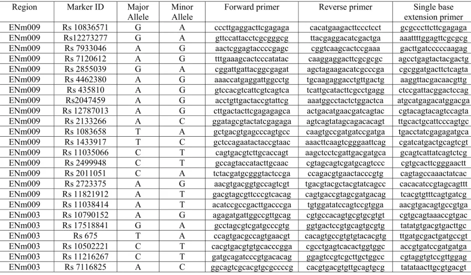
Selection of the markers

The major prerequisite for marker selection was heterozygosity for the particular donor. Initial preference of microsatellites was abandoned after inability to observe both single alleles in equal quantities in a set of 30 sperms. SNPs were selected as markers also due to a well-known fact that majority of them are biallelic (Petkovski et al. 2005).

Prior to marker selection the four Encode regions were divided into 5 or 9 (depending on the size of the region) 100 kb intervals. The preference for the length of the interval was based on assumption that the regions have intermediate recombination rate of 10

recombination events per bp and the following calculation:

For 1000 sperm cells: 10

*1000 = 10

events per bp. In order to recover at least 1 recombination event between adjacent SNPs, markers should be roughly located 10

bp or 100 kb away from each other.

As soon as the intervals were confirmed, all SNPs residing in intermediate zones of 5-7 kb between the intervals were downloaded from HapMap database. The preference was given to the SNPs with high allele frequency (close to 0.5:0.5 ratio) in the American Utah population of European origin (CEU) to increase the possibility to identify heterozygous markers.

Development of marker loci

The primers for 500 bp loci with allele of interest in the middle were developed using Primer3 program, ordered from Sigma-Aldrich, the loci were amplified by polymerase chain reaction.

Amplification of the marker loci

PCR was run using Qiagen Multiplex PCR Kit and 10 ng of high quality bulk sperm DNA. The

total reaction of 10 μl containing 5 μl of Qiagen Multiplex PCR Master Mix with HotStarTaq

DNA Polymerase and a unique PCR buffer containing the novel synthetic Factor MP (which

stabilizes specifically bound primers and enables efficient extension of all primers in the reaction

without optimization Ref: Qiagen Inc), 0.5 μl of forward and reverse primers, 1μl of bulk sperm

DNA and 3 μl of ddH

O. The reaction was run on Peltier Thermal Cycler (DNA Engine Tetrad2, BRB-Langertechnik GmbH) under the following cycling conditions:

Initial denaturation – 5 min at 96 ºC 30 cycles:

Denaturation: 30 sec at 95 ºC

Annealing: 45 sec at 50-70 ºC according to the T

of the primer Elongation: 1 min at 72 ºC

Final elongation: 5 min at 72 ºC

The PCR products were immediately run on 1% agarose gels containing EtBr and visually inspected for products under the UV light.

Purification of the PCR product

Before sequencing the PCR products were purified by Exonuclease I and Shrimp Alkaline Phosphatase. The clean up was conducted using the kit ExoSAP-IT (Affymetrix / USB).

ExoSAP-IT was added directly to the PCR product and incubated at 37 °C for 15 min. After PCR treatment, ExoSAP-IT was inactivated simply by heating to 80°C for 15 min.

DNA sequencing

The DNA products were sequenced directly, using the same primers as for PCR. Samples for both marker and haplotype confirmation were sequenced at the sequencing service facility of Cologne Center for Genomics at the Institute for Genetics, Cologne in an Applied Biosystems 3730 capillary DNA analyzer.

Sequencing reaction was performed using Big Dye Terminator Sequencing Kit version 3.1 (ABI,

Applied Biosystems, Foster City USA) according to the manufacturer protocol in a total volume

of 10 μL :

10 μM sequencing primer – 0.5 μl 10-30 ng purified PCR product Sequencing Buffer - 2 μl Big Dye Terminator – 2 μl ddH

O to 10 μl final volume

The reactions were run in a GeneAmp PCR System 9700 (ABI, Applied Biosystems) thermocycler under the following conditions:

Initial denaturation: 1 min at 96 ºC 40 cycles:

Denaturation: 10 sec. at 96 ºC Annealing: 15 sec at 50 ºC Elongation: 4 min at 60 ºC Final elongation: 5 min at 72 ºC

Reactions were stored at 12 ºC. Prior to capillary analysis 10 μl of ddH

O was added to every

sample (total 20 μl volume). The output trace files were analyzed with FinchTV software.

Haplotype screen

The initial haplotype screen over 2.5 Mb total of 4 Encode regions flanked by 48 SNP markers (2 SNPs per locus, total 25 loci of interest) was performed by using 48 GenomeLab SNPstream (Beckman Coulter, California, USA) at Cologne Center for Genomics. All materials (SNP ware reagent kits, mastermixes, etc) and services (primer development, software) were provided by Beckman Coulter, Inc.

After confirmation of the heterozygous markers, primers were developed and ordered.

After whole genome amplification cells were diluted 1:8 and 1µl of the dilution (20-100 ng of the amplificon) were used for the SNPstream screen. The samples were placed in 384-well plates.

Total of 1536 single cells were analyzed.

Principle of SNPstream

Using the SNPstream system (Beckman Coulter), multiplex genotyping can be performed in a 384-well microtiter plate format (Syvänen, 2005). SNPs with the same nucleotide variation are combined into multiplex reactions with 12 - 48 SNPs per reaction. Thus, up to 48 SNPs can be genotyped in 384 samples to generate a maximum of 18,400 genotypes on a single plate.

Following multiplex PCR, the remaining primers and dNTPs are inactivated enzymatically by Exonuclease I and shrimp alkaline phosphatase treatment. Cyclic minisequencing reactions are performed in solution using primers with 5’-Tag sequences and fluorescent ddNTPs, labelled with Tamra for one allele and Fluorescein for the other (Bell et al. 2002). The minisequencing reaction products are captured by hybridisation to complementary Tag-sequence immobilised on thebottom of 384-well glass plates.

The fluorescent nucleotides incorporated into the primers are detected using the CCD camera of the SNPstream system (Bell et al. 2002). The fluorescence signals from each sample are extracted from the images and displayed in a scatter plot where three clusters define a homozygous or a heterozygous genotype for each sample (Fig. 37, Appendix).

SNPstream procedure

The first stage of SNPstream analysis consisted of 48-plex PCR reaction for every sample provided with 96 unique primers per every reaction. PCR conditions:

Initial denaturation: 1 min at 94 ºC 39 cycles:

Denaturation: 30 sec. at 94 ºC

Annealing: 30 sec at 55 ºC Elongation: 1 min at 72 ºC 4 ºC final hold temperature

Following PCR each sample was treated with 3 μl of SBE clean up reagent (USB, Inc), consisting of Endonuclease 1 and Shrimp Alkaline Phosphatase mixture. Then the 384-well plates were sealed with Microseal A film and incubated on PTC-225 Tetrad at 37 ºC for 30 min.

A final incubation at 100 º C ensured complete inactivation of the enzymes.

The second stage consisted of single base primer extension. The primers were developed and ordered together with multiplex PCR primers. Special extension mastermix was provided by Beckman Coulter. 7 μl of the mastermix were added to every sample. Then the plates were sealed and thermal cycled according to the following protocol:

Initial denaturation: 3 min at 96 ºC 45 cycles:

Denaturation: 20 sec. at 94 ºC Annealing: 11 sec at 40 ºC 4 ºC final hold temperature

After the extension step, 48-plex SNPware plates were washed with Wash Buffer 1 (diluted in 1:20 in ddH

O).

The third stage was hybridization. 10 μl of hybridization solution (SNPware hybridization,

Beckman Coulter) were added to each well. The SNPware plates were sealed and incubated at 42

ºC for two hours at close to 100% humidity. During this time extension products were hybridized

to specific microarray spots on the bottom of the plate with specific tags. After the incubation, the

plates were washed with Wash buffer 2 and dried by inverting in a Beckman Coulter TJ-25

centrofuge and spinning at 1000 x g for 3 minutes. The SNPware plates were then imaged on the SNPstream Imager for duration of 7 minutes.

The forth stage was to capture data from SNPware plate by the Run Manager software module and transfer as raw images to the image application (Syvänen 2005). The image software module analyzed the images from the each well and determined the positions of the microarray spots to assess individual spot quality and extract their average intensity values. These data were uploaded to the SNPstream database and then combined with the sample set up data (Syvänen 2005). The GetGenos/QC review converted the numbers and sample position data into scatter plots, which were then automatically separated into statistical genotype clusters (Fig. 37, Appendix). Genotype clusters passing user-definable quality parameters were accepted and the genotypes were exported into a result file generated by the Report module.

Allele confirmation

Samples showing the recombinant haplotype were assessed and additional markers were selected to confirm them. The main criterion for these markers was heterozygosity condition and location as close to the initial marker as possible.

Primers for initial and nested PCR were developed with Primer3 software and ordered from Sigma-Aldrich. The loci containing allele of interest in the middle were 500 bp long for first PCR and 250 for the nested.

The products of whole genome amplification were diluted 1:2 and 1 μl (5-10 ng) were used for amplification of the marker loci.

PCR was run using Qiagen Multiplex PCR Kit and 10 ng of high quality bulk sperm DNA. The

total reaction of 10 μl containing 5 μl of Qiagen Multiplex PCR Master Mix with HotStarTaq

DNA Polymerase and a unique PCR buffer containing the novel synthetic Factor MP (which

stabilizes specifically bound primers and enables efficient extension of all primers in the reaction

without optimization Ref: Qiagen Inc), 0.5 μl of forward and reverse primers (10 μM – 0.5 ml), 1

μl of single sperm DNA and 3 μl of ddH

O. The reaction was run on Peltier Thermal Cycler

(DNA Engine Tetrad2, BRB-Langertechnik GmbH) under the following cycling conditions:

Initial denaturation – 5 min at 96 ºC 30 cycles:

Denaturation: 30 sec at 95 º C

Annealing: 45 sec at 50-70 ºC according to the T

of the primer Elongation: 1 min at 72 ºC

Final elongation: 5 min at 72 º C

The PCR products were immediately run on the 1% agarose gels containing EtBr and visually inspected for products under the UV light.

In case of product absence on the gel, a nested PCR was performed using ordered nested primers.

The total reaction consisted of 10 μl containing 5 μl of Qiagen Multiplex PCR Master Mix, forward and reverse primers (10 μM – 0.5 mL), 1 μl of single sperm DNA and 3 μl of ddH

O.

The reaction was run on Peltier Thermal Cycler (DNA Engine Tetrad2, BRB-Langertechnik GmbH) under the following cycling conditions:

Initial denaturation – 5 min at 96 º C 30 cycles:

Denaturation: 30 sec at 95 ºC

Annealing: 45 sec at 50-70 º C according to the T

of the primer Elongation: 1 min at 72 ºC

Final elongation: 5 min at 72 ºC

The PCR products were immediately run on 1% agarose gels containing EtBr and visually inspected for products under the UV light.

Purification of the PCR products and DNA sequencing were conducted the same way as

descriped on page 23.

Buffers

HOM (homogenizing buffer) 160 mM Sucrose

80 mM EDTA (ph 8.0)

100 mM Tris (ph 8.0)

0.5 % SDS

0.10 mg/ml Proteinase K

10x PBS (phosphate buffered saline) 1.3 M NaCl 70 mM Na

HPO

30 mM NaH

PO

pH 7.2

TAE (tris/acentic acid/EDTA) buffer 40 mM Tris, ph 8.5 2 mM EDTA

0.114 % glacial acetic acid

TE (tris/ EDTA) 10 mM Tris – HCl

2 mM EDTA

2.2. Theoretical methods

Correlation between nucleotide diversity and recombination rate

9.4 Million human SNPs were extracted from SNPdb (for the years 1998, 1999, 2000, 2001, 2002, 2003, 2004) at NCBI and analyzed according to their entry date, validation status, chromosomal location and compared their genomic positions with available recombination maps (Dib et al., 1996; Yu et al., 2001; and Kong et al., 2002). Recombination rates are given for bins of 1MB. Therefore, this bin size was used to determine SNP density by accumulating the number of SNPs within each bin. Heterozygosity was estimated from SNP density and average sample size within each bin (Watterson's estimate of theta, Waterson, 1975):

Where S is a number of the segregating sites and n is a sample size Displaying obtained data

Conversion and cross over data, as well as data on 13-mer degenerate motif and core motif (Myers et al, 2008) were displayed as custom annotation tracks in the UCSC genome browser (https://cgwb.nci.nih.gov/goldenPath/help/customTrack.html). All files were organized in “BED”

format and displayed either as BED lines (conversion tracts and motif) or as BED wiggle (fine scale recombination rates from International HapMap Consortium, 2003 and 2005).

SNP density (for four Encode regions) was expressed as an average number of SNPs in a one or fifty kb sequence.

The CG content percentage of the conversion tracts was calculated as:

[ (G+C)/(A+T+G+C)] ×100

Expected and observed CpG fraction was calculated for conversion tracts as well.

3. Results

3. 1 Recombination and variability in public data

To investigate the presence of a correlation between variation data and recombination, human SNPs (bulk genome-wide data, year 1999-2004, roughly 9.4 million) were downloaded from dbSNP and analyzed according to entry date, validation status and chromosomal location. They were also compared to genomic positions with available recombination maps from Genethon (Dib et al. 1996), deCode (Kong et al. 2002) and Marshfield Center (Yu et al. 2001).

First, SNP density for the two sets of SNPs was plotted against recombination rate (deCode, sex- average, 2002). The first set contained all available SNPs from SNPdb, the second contained the set of SNPs with a defined validation status (Fig.6).

Fig.6. Scatterplot of recombination rate (deCode) and SNP density based on data from SNPdb, build 124 (2004). Correlation coefficient for all SNPs is r = 0.15 and, for validated SNPs, r = 0.28. The red and the blue lines indicate the regression lines for the two data sets.

In the case of whole genome bulk data, the correlation coefficient between SNP density and

recombination rate was r = 0.15. When only validated SNPs (those, for which the validation

status in the database was higher or equal to 2; validated SNPs have annotated experimental

evidence, which confirms that the particular SNP is not a sequencing error) are considered, the

observed correlation became stronger (r = 0.28). However, the picture changed when a different

measure of variability was compared to the recombination map. Heterozygosity (SNP density

corrected by the sample size) plotted against the recombination map revealed either weaker

correlation (r = 0.14) compared to SNP density in the case of validated SNPs, or even negative correlation when bulk data (all SNPs with available sample size) were considered. Thus, these data did not support the initial expectation that positive correlation would be present independent of the quality and quantity of the SNP sets. The possible explanation for this observation is higher sample size of SNPs in the higher recombining regions of functional interest (e.g., major histocompatibility complex – MHC). In such regions of increased diversity and recombination rate, correlation coefficient (based on data up to 2004) was strongly positive, whereas the strength of correlation on the genome-wide scale was weakly positive or negative due to incomplete sampling in non-functional genomic regions.

Fig. 7. Scatterplot of the recombination rate (deCode) and heterozygosity based on data from SNPdb, build 124 (2004). Correlation coefficient for all SNPs is r = -0.03 and for validated SNPs r = 0.14. The red and the blue lines indicate the regression lines for the two data sets.

The strength of correlation varied on both broad- and fine-scale levels. The correlation coefficient

varied greatly when SNP density, as well as recombination rate was plotted for each chromosome

separately (Fig.8).

Fig.8. Correlation coefficient between SNP density and recombination rate for each chromosome (SNPdb, build 124 and deCode recombination map).

Again, there was no consistency between the bulk SNPs coefficient and the coefficient calculated for validated SNPs. Coefficients were in agreement only for chromosomes 3 and Y. Chromosome 9 shows a good example of sampling bias due to the discrepancy of correlation coefficients for two different data sets (Fig.8). Correlation is strongly positive for validated SNPs and negative for all available SNPs (SNPdb, build 124) on the chromosome.

The magnitude of correlation between SNP density and recombination rate changed across years as well (Fig. 9). SNP data from 1998 and 1999 were scarce and did not uniformly cover the entire genome. Starting from 2000, the accumulation of SNPs was accompanied by a decrease in the correlation coefficient, which could be due to the availability of higher resolution recombination maps, while resolution of SNPs lagged behind. With additional sequencing data from 2003 and 2004, the correlation coefficient increased. Another reason for the coefficient decline could be the change in sample size (number of chromosome investigated per SNP). From 1998 up to 2002 the sample size per SNP has increased, but the correlation coefficient seemed to decline.

X  Y 

Fig.9. Correlation Coefficient between nucleotide density and recombination rate across seven years, all SNPs from SNPdb, build 124 (2004).

The strength of correlation between SNP density and recombination rate also depends on the

recombination map. Fig.10 shows how the magnitude of correlation varied with the different

recombination data while SNP density remained the same. Up to 2004 both precision and

resolution of these maps were of low quality (Genethon, DeCode and Marshfield genetic maps

were estimated from pedigree studies with resolution at the CentiMorgan scale from 1 to 2 MB,

although recombination rates are known to vary at the kilobase scale – Spencer et al., 2006) and,

thus, their reliability is questionable.

Fig.10. Correlation coefficient plotted for different recombination maps across the years

Data available from 2005 and later, after the HapMap project had started, provided a better resolution and a larger sample size and was assumed to give better insights into the observed correlations. The plot of SNP density and fine scale recombination rates from Phase 1 of the HapMap project revealed a negative correlation between the SNP density and recombination map (McVean et al 2004; Fig.11).

Generation of additional HapMap data sets (Phase 1 and 2) starting from 2006 provided new

insights into the correlation between SNP density and recombination rate. Fig.11 shows the

correlation between SNP density and recombination rate on chromosome 11; the extracted data is

from 2008. The correlation coefficient is markedly weak (r =0.029) and when compared to the

plot with correlation magnitude for chromosome 11 across the years, the decrease in correlation

strength is obvious. Similar observations for 1998 – 2002 in correlation magnitude leads to the

hypothesis that generation of new data are accompanied with decrease in coefficient strength.

These observations of correlation strength discrepancy in 1998-2002 compared to the period of 2002-2004 can raise a question of what is a “true signal” and whether strong positive correlation was indeed observed or was this observation due to incomplete data?

According to the higher resolution data, such a correlation decrease with arrival of a new dataset can again indicate that incomplete sampling and prevalence of SNPs from functional highly recombining regions was the possible reason to observe strong positive correlation on the genome-wide scale.

Recombination data used in this analysis were obtained mainly from broad-scale maps (Dib et al.

1996, Yu et al. 2001, Kong et al. 2002) based on population genetic data, which were scarce at

the beginning of the century. Although the current data set from HapMap is of much better

resolution, the highest possible resolution can only be achieved by direct experiments. The

experimental approach of single-sperm typing was modified according to available facilities and

conducted to study current individual (not population-wide) cross over rates. Sperm typing was

performed for four Encode regions on chromosome 11. The following chapter demonstrates why

chromosome 11 and four Encode regions were selected to investigate cross over and gene

conversion rates.

Fig.11. Correlation between SNP density and recombination rate. Both SNPs and recombination rates were obtained from HapMap (A haplotype map of human genome, 2005).

The correlation coefficient r = -0.094. Recombination rates come from finer scale data (per base pair)

Fig.12. Correlation between SNP density and recombination rate for chromosome 11

(Conrad et al., 2006). The correlation coefficient r = 0.029. Recombination rates come from

broad scale data (centiMorgan per Megabase).

3.2 Specificity of sperm sorting on FACSVantage SE Cell Sorter

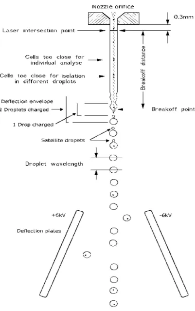
In sorting experiments, purity, yield, sorting speed, and count accuracy must be balanced depending on the desired outcome. The critical point for sperm sorting on a typical FACSVantage SE system is to setup an appropriate drop-delay.

The drop-delay is the time it takes for a cell to travel between the laser intersection point down to the end of the liquid jet before the jet breaks off in droplets (breakoff distance, Fig.13). At the laser intersection point, the optical cell parameters are measured. If the cell fulfills the sorting criteria, a voltage pulse is generated after the drop-delay and applied to the liquid jet during the separation of the droplet from the liquid jet. Thus, the droplet containing the cell is charged and ready for deflection in a static electric field generated by two deflection plates. If the drop delay setting is incorrect, droplets are charged at the wrong time and the sorter deflects empty droplets or droplets with erroneous cells at great precision. To set up the desired drop-delay, a sample with fluorescent beads is run through the sorter. This configuration is called “AccuDrop” and it is indispensable for single cell sorting. A sorting window is set in such a way that all beads are included and sorted to the deflected droplet stream. A fluorescence emission filter is moved in front of the video camera to block the laser light (the camera is attached under the deflection plates to illuminate the deflected and un-deflected droplet stream). On the monitor one or two fluorescence spots can be visualized from the fluorescent beads inside the droplets. With the right drop-delay setting no fluorescence should be detected in the un-deflected droplet stream. By watching the monitor and adjusting the drop-delay setting up or down, an optimal value for the drop-delay can be found. The fluorescence spot from the deflected droplet stream should be as bright as possible and other spots as dark as possible. As an example, the AccuDrop method is sufficient for sorting of embryonic cells (Shapiro, 2003).

Sperm cells require a better optimized drop-delay setting due to certain morphological peculiarities. The tail position (straight or curled) and smooth shape of the cell change the fixed speed necessary to cover the break off distance, even with the AccuDrop method. Also, they tend to form clumps and often arrive too close together to be individually sorted. In this case, droplets containing particles are aborted and replaced by empty droplets in the plate well (Shapiro, 2003).

The optimal drop-delay option can be determined by performing a Drop Delay Profile (Table 1).

For this procedure, a specified number of droplets (for instance, 20) are sorted onto a microscope

slide at different drop-delay settings. This procedure requires the use of a fluorescent microscope

and the pre-staining of sperm with Hoechst flourochrome. It begins with the lowest drop-delay from the bead sorting and this value is increased at each iteration by as low as 0.1 drops (Table 1). The setting that provides the highest sperm count is the optimal drop-delay setting.

Fig 13. The sketch of a sorting nozzle (Shapiro 2003).

Table 1. Example of a drop delay profile in a sperm sorting experiment using FACSVantage SE sorting system.

drop- delay

-0.3 -0.2 -0.1 AccuDrop measurement

19.1

+0.1 +0.2 +0.3 +0.4 +0.5

Sperm cells count

- 1 5 10 11 19 19 20 20

*

- optimal setting determined by AccuDrop method for the particular experiment prior profile start.

3.3 Estimation of the cross over rate:

According to the hotspot detection strategy by single-sperm analysis (Arnheim et al., 2003): if a pair of markers flanking the interval of interest is 1 Mb in size, then 1% of sperm are expected to have a recombinant haplotype for these two markers, assuming that recombination rate is average.

Expected cross over rate in all four regions. Considering the length of every interval flanked by two markers in this study (all Encode region were divided into intervals of 100kb) and the sample size of sperm (1000 single cells), 0.1% of sperm are expected to have recombinant haplotypes within every interval. In all four Encode regions (2.5 Mb long), 25 recombinant haplotypes are expected in total if 1000 sperm cells are typed.

Expected cross over rate per region. According to theoretical expectation based on the

assumption that the average rate is 1 cM/Mb (Arnheim et al., 2003), 0.1% of cells are expected to

have recombinant haplotypes per every 100 kb interval. Three out of four Encode regions

(ENr332, ENm003, ENr312) 0.5 Mb long will be expected to have 0.5% of recombinant

haplotypes. In the sample of 1000 sperm, each of these three regions is expected to have five

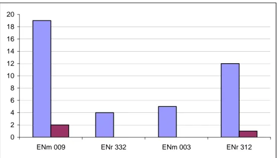
recombinants. ENm009, which is 1 Mb long, is expected to have 10 recombinants. According to the population data expectation (LD-based, deCode map, UCSC browser), the average recombination rates per region are 1.95 (ENm009), 0.9 (ENr332), 1 (ENm003) and 2.5 (ENr312) cM/Mb. Fig. 14 shows the comparison of the expected (LD-based, broad scale) with the observed (experimental) cross over events.

Observed cross over rate in four regions. In this study, only three cross over events were identified experimentally, which makes the cross over rate (considering the total sample of 1000 cells) 0.3% per 2.5 Mb. For every 1 Mb of these 2.5 Mb, the rate is 0.12 %. Thus, the final estimate is 0.12 cM/Mb.

0 2 4 6 8 10 12 14 16 18 20

ENm 009 ENr 332 ENm 003 ENr 312

Fig. 14. Expected (from population data from DeCode map) versus observed (experimental)

number of cross over events per Encode region. Knowing the average recombination rates per

Encode region (deCode map, UCSC browser) 1.95, 0.9, 1 and 2.5 cM/Mb, the numbers of

expected cross over events per region were calculated as 19, 4, 5 and 12, respectively. Observed

number of cross over events were 2 in ENm009 and 1 in ENr312. The expected amount of cross

overs is shown in blue and observed amount is in red.