Two-stage methods for multimodal optimization

Two-stage Methods for Multimodal Optimization

Dissertation

zur Erlangung des Grades eines

D o k t o r s d e r N a t u r w i s s e n s c h a f t e n der Technischen Universität Dortmund

an der Fakultät für Informatik von

Simon Wessing

Dortmund

2015

1. 7. 2015 Dekan:

Prof. Dr.-Ing. Gernot A. Fink Gutachter:

Prof. Dr. Günter Rudolph, Technische Universität Dortmund

Jun.-Prof. Dr. Tobias Glasmachers, Ruhr-Universität Bochum

Contents

1 Introduction 5

1.1 Problem Statement . . . . 6

1.2 Average Case versus Worst Case . . . . 8

1.3 The Two-stage Optimization Paradigm . . . . 10

1.4 Distances and Neighbors . . . . 13

1.5 Objectives of this Work . . . . 14

2 Benchmarking 17 2.1 Quality Indicators for Multimodal Optimization . . . . 17

2.1.1 Diversity Indicators . . . . 17

2.1.2 Discussion of Diversity Indicators . . . . 25

2.1.3 Other Quality Indicators . . . . 27

2.1.4 Discussion of Other Quality Indicators . . . . 32

2.2 Performance Measurement . . . . 33

2.3 Test Problems . . . . 36

2.3.1 Multiple Peaks Model 2 . . . . 38

2.4 Experimentation . . . . 41

3 Summary Characteristics for the Assessment of Experimental Designs 45 3.1 Low-dimensional Projections . . . . 46

3.2 Irregularity . . . . 47

3.3 Distance to the Boundary . . . . 48

3.4 Distance between Center of Mass and Centroid of the Hypercube . . 50

3.5 Testing the Linear-time Indicators . . . . 51

3.6 Other Criteria for Experimental Designs . . . . 52

4 Sampling 55 4.1 Latin Hypercube Designs . . . . 55

4.1.1 Fast Improved Latin Hypercube Sampling . . . . 58

4.2 Quasirandom Sequences . . . . 60

4.3 Subset Selection Methods . . . . 63

4.3.1 Part and Select Algorithm . . . . 64

4.4 Point Processes . . . . 69

4.4.1 MacQueen’s Algorithm . . . . 70

4.4.2 Maximin Reconstruction . . . . 70

4.5 Comparison of Sampling Methods . . . . 76

4.5.1 Experiment on Sampling Algorithms . . . . 77

5 Optimization 85

5.1 Restarted Local Search . . . . 86

5.1.1 Experiment on Restarted Local Search . . . . 87

5.2 Clustering Methods . . . . 94

5.2.1 Utilizing Nearest-better Distances . . . . 95

5.2.2 Experiment on Clustering Methods . . . 100

5.3 Comparison of the Optimization Algorithms . . . 112

6 Conclusions and Outlook 117

Glossary 123

List of Figures 127

List of Tables 129

List of Algorithms 131

Bibliography 133

1 Introduction

The need of obtaining a set of good solutions in contrast to a single globally opti- mal solution of a multimodal problem is often mentioned in discussions of practical optimization [14, 1, 95]. The rationale behind this opinion is that a decision maker may have additional criteria to consider, which are not included in the optimization problem [14]. Such criteria may be side constraints or additional objective functions, and there may be various reasons not to incorporate them in the optimization prob- lem. One argument is that different objectives could be incommensurable (e. g., in general, time is not money), and thus should not be aggregated into one function.

In this case, a multiobjective problem formulation would be possible and probably appropriate [14]. However, sometimes this approach is not feasible because the ex- pert knowledge constituting the additional criteria has not been formalized or the evaluation is more or less subjective. Then, it is often stated only informally that an optimization algorithm should be able to produce several different solutions of good quality for the formalized objective [1].

It is also possible that the objective functions of a multiobjective problem are very heterogeneous [52]. For example, one objective function could be multimodal and the other only linear. Such a situation could, e. g., appear if the first function evaluates the features of a product by running a computationally expensive simulator or doing physical experiments, and the second simply represents the production costs. This also implies that the former objective is a black box, while the latter one is available in analytical form. In summary, one objective may be more difficult than the other one in practically every regard. In this case it seems advisable to focus on the more difficult multimodal function with a single-objective approach. The linear function could perhaps be used for narrowing down the region of interest, but otherwise it would probably only appear in the post-processing of the solution set obtained from the optimization of the first objective. So, this set should possess a high diversity in decision space, to enable different evaluations according to the remaining criteria.

Another more specific example, where the task of identifying several local optima

appears as an internal subproblem, are model-based optimization (MBO) algorithms

that want to employ parallelization. In model-based optimization, a meta-model

f(x) is built from a finite number of tuples (x, f ˆ (x)), where x is a point in the

domain of f , and f(x) is its associated objective value. The model is then used

to determine one or more locations for the next exact evaluations of the objective

function f . The goodness of a location is assessed with a so-called infill criterion,

which is typically a multimodal function. For a batch-sequential version of the MBO

algorithm, several distinct optima of the multimodal infill criterion have to be ap-

proximated per iteration [138, 19]. Although this work does not directly deal with

meta-modeling, we will encounter several references to this field, because we are borrowing ideas from it. Likewise, some of the methods developed here should also be relevant for meta-modeling.

The area containing single-objective problems with the need to identify a set of solutions is nowadays called multimodal optimization (MMO) in the area of evo- lutionary computation. The term may have been originally coined by Beasley et al. [14], probably as a short form of “multimodal function optimization”, as used by Goldberg and Richardson [50]. In this work we want to formally define MMO, corresponding performance measures, and explicitly assess optimization algorithms under the objective of obtaining a set of good local optima.

1.1 Problem Statement

In the following, we will assume to have a deterministic objective function f : X → R , where X = [ℓ, u] ⊂ R

is the search space or region of interest (ROI) and n ∈ N is the fixed number of decision variables. The vectors ℓ = (ℓ

, . . . , ℓ

)

and u = (u

, . . . , u

)

are called the lower and upper bounds of X , respectively. The function f is assumed to be multimodal and analytically unknown. Naturally, also analytic gradient information is not available in this case. For these reasons we call f a black-box function.

Although they did not use the name yet, a multimodal optimization problem is in principle already defined by Törn and Žilinskas [143, pp. 2–3]. The following definition is based on their formulations.

Definition 1 (Multimodal minimization problem). Let there be ν local minima f

, . . . , f

of f in X . If the ordering of these optima is f

< · · · < f

< h < · · · <

f

, a multimodal minimization problem is given as the task to approximate the set S

i=1

X

, where X

= { x ∈ X | f (x) = f

} .

The variable h in this definition is simply a threshold to potentially exclude some of the worse optima. For simplicity, we will always assume h = ∞ in this work, so we will be interested in all local optima of a problem. This case is described in [114, Sec. 5.1] as the task of recovering “all known” optima of a test problem.

Global optimization can be seen as a special case of multimodal optimization, where

we are only interested in finding the X

corresponding to the global optimum

f

= f

. This problem is closely related to the black-box levelset approximation

problem [40]. However, usually it is sufficient to find just one x

∈ X

in practical

applications referring to global optimization. Even this problem is mathematically

unsolvable [143, p. 6]. Therefore, we will take a pragmatic approach to the problem

by trying to obtain the best possible performance (as defined in Section 2.1.3) with

restricted resources, i. e., a finite number of objective function evaluations. Further

assumptions concern the properties of the objective function: We will restrict our

considerations to problems for which a positive constant ε can be specified, so that

the distance between any two optimal positions is larger than ε. This implies a finite

1.1 Problem Statement number of optimal positions [119], so we could alternatively formulate the problem as the task to find the k best optimal positions of the objective function. It also means that each optimal position is surrounded by its own attraction basin.

Definition 2 (Attraction basin, [141]). For the position x

∈ X of an optimum, basin(x

) ⊆ X is the largest set of points such that for any starting point x ∈ basin(x

) the infinitely small step steepest descent algorithm will converge to x

.

Realistic functions should possess some smoothness, that is, the probability p

= vol(basin(x

))/ vol( X ) to find x

with an ideal descent algorithm started from a ran- dom uniform point should be significantly greater than zero [143, pp. 7–10]. Here, vol( · ) denotes the Lebesgue measure of the sets [18, pp. 171–181] and p

obviously is the relative size of an attraction basin in comparison to the whole search space.

In this simplified model, the probability of finding x

can naturally be amplified by carrying out N local searches from random uniform starting points. The correspond- ing formula for this probability P reads P = 1 − (1 − p

)

[143, p. 86]. By solving for N , we obtain the estimate

N =

ln(1 − P ) ln(1 − p

)

(1.1) as the required number of points for finding x

with probability P [140]. The strong influence of p

on the problem difficulty can be illustrated by inserting some numbers into (1.1): if we require P = 0.95 and assume p

= 0.01, the equation yields N = 299.

Decreasing p

by a factor increases N by the same factor, e. g., a value of p

= 0.001 already results in N = 2995. The problem of obtaining all optima is of course generally more difficult and also the math for estimating the corresponding numbers becomes more complicated. For details, we refer to [114, Sec. 3.3].

The cost of one objective function evaluation is another important property of the problem, as it decides on the number of possible function evaluations. In this work, we assume that this cost is constant, i. e., all function evaluations cost the same. The number of function evaluations in turn influences how much computational effort should be invested to determine the location of the tested points. If only very few function evaluations can be afforded, the amount of additional computations may be very high, because sample locations must be chosen carefully. The assumed budgets in the literature vary widely and have considerable influence on which optimization algorithm obtains a good performance or is even applicable.

Table 1.1 shows how some budgets are associated with research areas and appli-

cations. The interesting budgets for this work are highlighted in lime green. This

focus has been set by subjectively considering what may be possible in real-world

optimization, e. g., for design problems in engineering, and what is manageable in

benchmarking. This is also a setting where the common black-box optimization

benchmarking (BBOB) practice [44] of measuring consumed resources simply as the

number of objective function evaluations seems still admissible, as the assumption

of expensive function evaluations in relation to the overhead of an optimization al-

gorithm becomes rather unlikely with larger budgets [38]. If budgets are smaller,

Table 1.1: Different magnitudes for the number of function evaluations N

. Magnitude Application

n · 10

Initial designs in model-based optimization [70]

n · 10

Expensive optimization n · 10

n · 10

Budget of the CEC 2005 competition [135]

n · 10

n · 10

Budget of the black-box optimization benchmark (BBOB) [44]

then probably meta-models should be used [70] and more emphasis should be put on parallelization, if possible.

Törn and Žilinskas [143, p. 93] write

“[. . . ] one can expect that the practitioner would undertake a large num- ber of experiments in order to be convinced that the problem is thor- oughly analyzed. The optimization would hardly be stopped until all research resources have been spent.”

This quotation shall serve as justification to consider a fixed-budget scenario, i. e., measuring optimization performance after a certain amount of resources has been spent. (Although this does not mean that only a single fixed budget size is investi- gated.)

1.2 Average Case versus Worst Case

A large part of this work deals with (uniform) sampling algorithms and the prop-

erties of the point sets produced by them. Some examples of such point sets are

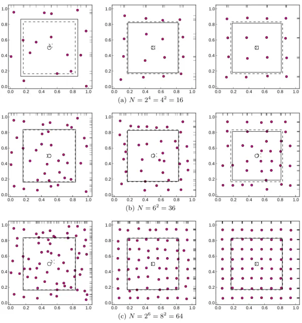
presented in Figure 1.1. With exception of Figure 1.1d with N = 120, each set con-

tains N = 121 points. (The corresponding algorithms will be discussed in Chapter 4.)

One permissible quality feature is the distribution of one-dimensional projections of

the points, which should be as uniform as possible. The set in Figure 1.1d (taken

from [12]) is perfect in this regard. Another important feature is the uniformity in

the original, high-dimensional space. In Section 4.2 we will see that deterministic

quasirandom sequences (as in Figure 1.1b) with low discrepancy (i. e., low devia-

tion from uniformity) provide a worst-case error bound for the integration error

in numerical integration. Corresponding randomized variants provide a variance re-

duction compared to random uniform sampling (Figure 1.1a) [88]. These results are

relevant for global and multimodal optimization, because estimating the size of an

attraction basin is nothing more but numerical integration. In practice, we are of

course not interested in the actual basin size, but simply in discovering all existing

basins, and thus all existing optima. This requirement is also served, because reduc-

ing the variance of basin size estimates encompasses reducing the risk of missing any

1.2 Average Case versus Worst Case

0.0 0.2 0.4 0.6 0.8 1.0

0.0 0.2 0.4 0.6 0.8 1.0

(a) Random uniform

0.0 0.2 0.4 0.6 0.8 1.0

0.0 0.2 0.4 0.6 0.8 1.0

(b) Halton sequence

0.0 0.2 0.4 0.6 0.8 1.0

0.0 0.2 0.4 0.6 0.8 1.0

(c) Conventional grid

0.0 0.2 0.4 0.6 0.8 1.0

0.0 0.2 0.4 0.6 0.8 1.0

(d) Audze-Eglãjs LHS

0.0 0.2 0.4 0.6 0.8 1.0

0.0 0.2 0.4 0.6 0.8 1.0

(e) MmR+PEC,p= 1

0.0 0.2 0.4 0.6 0.8 1.0

0.0 0.2 0.4 0.6 0.8 1.0

(f) Sukharev grid

Figure 1.1: Examples of different sampling methods in two dimensions. One- dimensional projections of the points are indicated at the top and right axis. The cubes, cross, and circle indicate certain uniformity-related properties of the point sets, which will be explained in Chapter 3.

basin completely. Consequently, our multimodal optimization performance can be improved by employing variance reduction techniques, e. g., some kind of stratified sampling. Also Törn [140] argues that if we are using q strata, the required number of points N

to find optimum x

with probability P can be bounded by

q ln(1 − P ) ln(1 − qp

)

≤ N

≤

ln(1 − P ) ln(1 − p

)

.

This result implies an improvement over random uniform sampling, because the upper bound is identical to (1.1).

However, theory predicts and experiments confirmed that variance reduction is

only possible for sufficiently smooth functions [100]. In case of high-frequency func-

tions, the performance of any uniform sampling method should be identical to that

of random uniform sampling [100]. In summary, this means that in a black-box sce-

nario, no deterioration of performance in comparison to random uniform sampling

is possible by using stratified sampling, as long as uniformity is ensured. Unfortu-

nately, creating and measuring uniformity in high dimensions is not as trivial as it

sounds (see Section 2.1.1 and Chapter 4).

0.0 0.2 0.4 0.6 0.8 1.0 0.0

0.2 0.4 0.6 0.8 1.0

0.00 0.12 0.24 0.36 0.48 0.60 0.72

0.0 0.2 0.4 0.6 0.8 1.0

0.0 0.2 0.4 0.6 0.8 1.0

0.0 0.1 0.2 0.3 0.4 0.5 0.6 0.7 0.8 0.9

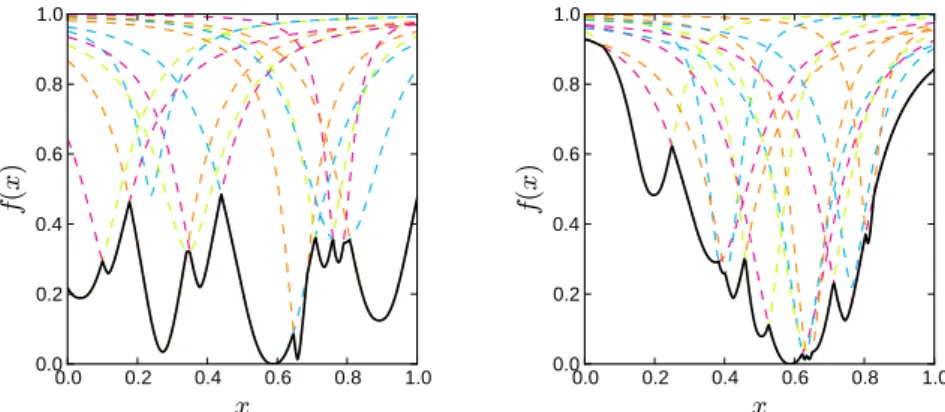
Figure 1.2: Examples of multimodal optimization problems with ν = 100 optima.

The left problem exhibits no global structure, the right one contains one large funnel. Every optimum is marked with a cross, the global one is encircled.

As soon as we begin sampling, the black-box assumption is weakened, because we are gaining more and more information about the problem. Special features of the global topology as the distribution of optima locations and the correlation of their objective values could be exploited to improve performance. The importance of the former aspect for problem difficulty was already recognized by Törn and Žilinskas [143, p. 11]. If we know, for example, that optima are embedded in a so called funnel structure [86] (see Figure 1.2), it would be advisable to deviate from uniformity and to sample with a higher density in better areas. By doing this, we are sacrificing the worst-case bound in favor of better average-case performance, and this is what is typically done in optimization [109], either by using local search or an adaptive sampling. The next section will elaborate on the kind of interplay between global and local approaches that is considered in this work.

1.3 The Two-stage Optimization Paradigm

Törn and Žilinskas [143, pp. 16–21] summarize several classification schemes of the early literature for global optimization algorithms. However, the criteria for these classifications seem often arbitrary and therefore no single ideal classification can be found. So, the approach here is to define a simple high-level concept that covers a large class of optimization algorithms. The proposed concept is based on the observation that many successful meta-heuristics are composed of several modules, which are quite sophisticated themselves. The complexity of these meta-heuristics often hinders the analysis of the individual components, i. e., it is difficult to assess how much influence a component has on the overall performance. Possibly the most simple representative of these compositions is that of two alternating stages [85].

Naturally, this idea is not restricted to multimodal optimization, but could, e. g.,

be also applied to multiobjective optimization or completely unrelated topics. And

1.3 The Two-stage Optimization Paradigm indeed, it has surfaced multiple times in different contexts. For example, Jones [69]

gives a survey of model-based two-stage methods for optimization. He distinguishes the two stages as follows:

1. Fit a response surface to training data (including estimation of the model’s parameters).

2. Use the surface to compute new search points under the assumption that the parameters are correct.

This approach has evolved from response surface methodology, which was originally applied to physical experiments (with a human in the loop) [34, pp. 7–11]. Another example is the restart variant of the covariance matrix adaptation evolution strat- egy (CMA-ES) [9]. The CMA-ES belongs to the class of evolutionary algorithms (EA), which are nature-inspired optimization methods [16]. They maintain a set of solutions during the optimization and create new candidate solutions by randomly combining and modifying the current ones. This process is typically described in the language of biology, by saying that a population of individuals is maintained and offspring are created from parent solutions by recombination and mutation. In each generation, the best individuals are selected to form the parent population of the next generation. The later development of the CMA-ES was driven by the question what to do in situations when the local search has converged, but part of the budget is still available. If the performance measurement does not reward savings in budget, a natural idea is to just restart the algorithm with a random starting point. In this case, the sampling of the random point trivially represents the other stage.

A “stage” can be defined abstractly as an algorithm that takes three inputs: the maximal number of function evaluations that may be consumed by this very call, a (possibly empty) set of individuals, and the optimization problem. We are using the terms individual and problem here instead of point and function, respectively, to indicate that we are dealing with objects that may contain additional meta- information. The object-oriented view emphasizes that the abstract concept can be instantiated in multiple ways. The outputs are another set of individuals and the consumed budget (the number of function evaluations actually used). The stage must assure that the maximal budget is never exceeded.

Törn and Žilinskas [143, p. 14] mention that most global optimization algorithms

consist of a global stage and a local stage. Although the distinction between these

two is rather fuzzy, it shall be a guiding theme of this work. Algorithm 1 sketches

a whole abstract two-stage method. It basically consists of a loop to ensure the

consumption of the whole budget and the two interacting stages in the loop. While

the code indicates that we enter the global stage before the local stage, this can be

the other way around as well. At the end of each iteration, an archive is updated

with the new individuals. This function is called “combine” to emphasize that it does

not necessarily have to be a set union. Also note that we define the communication

between the stages as being based on the exchanged individuals, in contrast to

Jones’ definition [69]. The algorithms he considered do in principle also match our

Algorithm 1 General two-stage optimization framework Input: budget B, archive A , problem F

Output: solution/approximation set

1:

while B > 0 do

2:

P , c

← globalStage(B, A , F )

3:

B ← B − c

// reduce budget by costs c

of global stage

4:

Q , c

← localStage(B, P , F )

5:

B ← B − c

// reduce budget by costs c

of local stage

6:

A ← combine( A , Q )

7:

end while

8:

return filter( A ) // potential subset selection definition, only the distinction to what he calls “one-stage” methods disappears.

Schoen [127] defines “two-phase” optimization methods in a very similar way as we do in Algorithm 1, but applies additional requirements to the local stage. First of all, an explicit local search algorithm has to be present. Secondly, he emphasizes that the local stage does not employ all the information available in A , but only certain selected starting points. This is also reflected in Algorithm 1 by giving the local stage the input P . Thirdly, he demands that no other information than the final result of the local search may be fed back to the global stage. While this last behavior often seems to be a convenient choice, because it focuses on the “high-quality information”, we do not necessarily want this property to be enforced.

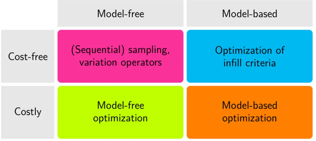
As already said, our definition encompasses a very broad class of algorithms, perhaps even to a point beyond recognition. For example, an evolutionary algorithm would fit into this paradigm if it uses both recombination and mutation. We could view the offspring creation by parent selection and recombination as the global stage, mutation and the evaluation of the offspring population as the local stage, and the survivor selection step as combination of A and Q . On the other hand, simulated annealing and an evolutionary algorithm without recombination would not fit into the two-stage paradigm [127]. However, the concept should be more interesting on a higher level anyway. Figure 1.3 makes a further categorization of stages into four groups. As in EAs, the global stage often does not use any evaluations of the objective function. Another such example would be a uniform sampling algorithm, which is also in the category of model-free, cost-free stages. The corresponding modules in model-based optimization are methods using infill criteria to determine candidate points. Stages with function evaluations are often whole optimization algorithms, although the consumed budget may vary greatly.

If one wants to emphasize the local-search aspect, the methods described by Jones

can only be classified as a module of a two-stage method, because they lack an

explicit local search and need relatively few function evaluations. However, also the

Restart-CMA-ES is a borderline case, because drawing a random uniform starting

point is just too trivial. As a compromise we can conclude that we are interested in

methods somewhere in between these two extremes.

1.4 Distances and Neighbors

Model-free Model-based

Cost-free (Sequential) sampling, variation operators

Optimization of infill criteria

Costly Model-free

optimization

Model-based optimization

Figure 1.3: Categorization of possible modules for global and local stages.

1.4 Distances and Neighbors

As already mentioned, sampling algorithms play an important role in this work. We will be dealing a lot with methods to generate point sets and methods to analyze their spatial properties (e. g., diversity). Thus, a core notion for us is the distance between two points. This distance is also a building block of many MMO performance measures and optimization algorithms.

Definition 3 (Minkowski distance, L

distance). The distance between two points x = (x

, . . . , x

)

∈ R

and y = (y

, . . . , y

)

∈ R

is defined as

d(x, y) = k x − y k

= X

| x

− y

|

!

.

For 1 ≤ p < ∞ , d(x, y) is a metric [18, p. 242]. However, it is seldom relevant for us that the Minkowski inequality (triangle inequality) d(x, z) ≤ d(x, y) + d(y, z) is violated for 0 < p < 1, so also these values are in principle possible choices for us. Other notable properties of distance metrics are non-negativity (d(x, y) ≥ 0), identity of indiscernibles (d(x, y) = 0 ⇔ x = y), and symmetry (d(x, y) = d(y, x)).

We will usually write d(x, y) to emphasize the independence of p, and k x − y k

if a certain p is assumed. If nothing else is said, the Euclidean distance with p = 2 is meant. Figure 1.4 shows some examples of distances for different values of p. In practice, we are often interested in short distances, that is, distances to neighbors of some point.

Definition 4. The distance to the nearest neighbor of x ∈ X in P ⊂ X , |P| < ∞ , is defined as

d

(x, P ) = min { d(x, y) | y ∈ P \ { x }} . (1.2)

The nearest neighbor itself shall be denoted nn(x, P ) and is obtained by using

arg min instead of min in (1.2). Throughout this work, P will always denote a discrete

0.0 0.2 0.4 0.6 0.8 1.0 0.0

0.2 0.4 0.6 0.8 1.0

0.0 0.3 0.6 0.9 1.2 1.5 1.8

(a)p= 0.5

0.0 0.2 0.4 0.6 0.8 1.0

0.0 0.2 0.4 0.6 0.8 1.0

0.00 0.15 0.30 0.45 0.60 0.75 0.90

(b)p= 1

0.0 0.2 0.4 0.6 0.8 1.0

0.0 0.2 0.4 0.6 0.8 1.0

0.00 0.08 0.16 0.24 0.32 0.40 0.48 0.56 0.64

(c)p= 2

Figure 1.4: Distances from (0.5, 0.5)

for different values of p.

set of points. Then, also the average distance to the k nearest neighbors may be a sensible characteristic.

Definition 5. Let y

, . . . , y

be the ordered elements of P , so that d(x, y

) ≤

· · · ≤ d(x, y

) for some x ∈ P / . Then, the average distance to the k nearest neigh- bors is denoted

d

(x, P , k) = 1 k

X

d(x, y

) .

Finding the nearest neighbors of points in R

is a common problem and sophisti- cated data structures exist to accelerate this task (cf. [151] for an overview). How- ever, these data structures are affected by the curse of dimensionality, which means that in high dimensions they yield no improvement over the naïve approach of enu- merating all neighbor candidates. Weber et al. [151] show experimentally, that the break-even point may already appear at only n = 10 dimensions. Related results of Beyer et al. [17] additionally show that under broad conditions, the difference between the Euclidean distances of a random uniform query point to its farthest and nearest neighbor in a point set vanishes with increasing dimension. This result puts a lot of doubt on approximate nearest neighbor data structures. Subsequently, Aggarwal et al. [5] found out that values of p ≤ 1 can prevent this effect. Their result serves as incentive to also investigate such distances in this work. However, doing so further hinders the use of acceleration techniques, as they typically require metric distances. Thus, we will only use the linear search through all points to find nearest neighbors.

1.5 Objectives of this Work

Two-stage optimization algorithms are an attractive concept for global and multi- modal optimization due to their simplicity and demonstrated performance [114, 2, 1].

Especially the Restart-CMA-ES has proved its competitiveness in global optimiza-

tion tasks [53]. The main focus of this work will be on improving the global stages,

as local search is already a thoroughly researched topic.

1.5 Objectives of this Work Although our investigations should also largely apply to global optimization, the primary interest of this work is in multimodal optimization, as it seems more challenging and interesting from a practical perspective. While meta-modeling and model-based optimization are not directly a part of the work, we will often discuss concepts with a view to them, because many requirements are shared between the areas. Model-based approaches would be especially promising on low-dimensional problems (e. g., n ≤ 10) with small budgets (e. g., N

≤ 10

n). For larger budgets, the approach is rather unattractive, because fitting the model becomes a run time bottleneck. However, there also is a big discrepancy between theory and practice in the area of small budgets: On the one hand, a lot of emphasis is put on using infill criteria that guarantee asymptotic convergence to the global optimum, on the other hand the considered budgets of function evaluations are extremely small.

As already indicated in Section 1.1, we will deal with larger budgets and conse- quently with model-free optimization algorithms. In summary, the following three research questions shall receive the most attention:

• How can performance be measured in multimodal optimization?

• Which is the best sampling algorithm according to the chosen performance measures, especially in high dimensions?

• How can the two two-stage approaches restarted local search and clustering method be improved and how do they perform in a comparison?

As most results in this work are experimental, we will establish the fundamentals for benchmarking in multimodal optimization in Chapter 2. This encompasses the definition of quality indicators, performance measures, and test problems. As the name implies, quality indicators are used for measuring the quality of the solutions to the optimization problem. A performance measure is usually regarded as something more general, especially incorporating the required time to obtain the solution. Test problems are required because real-world problems are too difficult to work with in large, controlled experiments.

In Chapter 3 we talk about useful characteristics of point sets designated for incorporation in the global stages of MMO algorithms. These characteristics as, e. g., diversity, irregularity, or the mean distance to the boundary are also highly related to space-filling experimental designs [126, pp. 121–161], which are an important building block for meta-modeling.

In Chapter 4, an overview of different sampling algorithms, collected from various

research disciplines, is given. Every algorithm is evaluated with appropriate sum-

mary characteristics of the previous chapters and two of them, namely improved

latin hypercube sampling and the part-and-select algorithm, are enhanced in terms

of run time. Finally, a new algorithm called maximin reconstruction (MmR) is pro-

posed, which has the advantage that it can be configured very flexibly. To conclude

the chapter, the most interesting algorithms are compared regarding their MMO

performance in a first basic experiment.

In Chapter 5, we finally arrive at the part of the work that deals with complete

two-stage optimization algorithms. After a short discussion of relevant approaches

in this area, two algorithm classes are investigated experimentally regarding their

improvability by using MmR as global stage, before the chapter is closed with a

comparison between the best variants of these two classes. Chapter 6 closes the

work with conclusions and an outlook.

2 Benchmarking

This chapter first surveys general diversity indicators and then specific quality indi- cators for multimodal optmization. Afterwards, it is discussed how these indicators can be incorporated into a performance assessment workflow for multimodal opti- mization. As we will see, there are some hidden pitfalls in the process that can cause misleading results. Then, an overview of artificial test problems is given, followed by a description of the test problem generator used for our experiments. The chap- ter concludes with some general remarks on experimentation, trying to explain the mindset that governed this work.

2.1 Quality Indicators for Multimodal Optimization

This section deals with measuring the quality of a multiset of points P ⊂ X with

|P| = N < ∞ . This set may for example be the result or the initialization of some optimization algorithm. While the diversity indicators in Section 2.1.1 are versatile in application, Section 2.1.3 deals especially with the assessment of the outcomes of multimodal optimization. The survey is an extended version of earlier ones in [117]

and [155].

With the denomination quality indicator, we exclusively mean unary quality indi- cators in this work, which are simply mappings from populations P to real numbers.

In other words, we could say that we are interested in numerical summary charac- teristics to describe P . The term indicator is used to show that the mathematical properties associated to metrics or measures are not necessarily given. The name is adopted from multiobjective optimization [160], because of its close similarity to MMO, especially concerning the virtues of a-posteriori methods. It should also be stressed that in the following, we will require that no gradient information and no additional function evaluations may be used for the assessment.

2.1.1 Diversity Indicators

Measuring the diversity of a multiset P is a common problem in many research areas.

We will encounter approaches from biology, physics, operations research, computer

experiments, and numerical integration. Although “diversity” is an abstract concept

and can mean different things, there are surprisingly many similarities between ap-

proaches that emerged from different applications. We will try to relate them to

each other by using a few axiomatic properties originating from Weitzman [152]. He

formulates several desirable properties for diversity measures, of which Solow and

Polasky [131] selected three that seemed especially natural to them. This subset has

also been adopted by Ulrich et al. [144]. As these requirements have been developed in the context of biological diversity, the term species is used for the elements of P in the following definitions. In our application, however, a species is simply some point x ∈ X ⊂ R

. Weitzman required neither the triangle inequality nor identity of indiscernibles for his axiomatic treatment. Instead of the latter one, the relaxed condition d(x, x) = 0 was assumed [152]. However, some of the diversity indicators in the following survey do assume the triangle inequality.

The consideres axioms are as follows:

Axiom 1 (Monotonicity in species). If a species t / ∈ P has a positive distance to all species in P , then adding it to P may not decrease the diversity:

∀ s ∈ P : d(s, t) > 0 ⇒ D( P ) ≤ D( P ∪ { t } ) .

Axiom 2 (Twin property TP1). Diversity should neither be increased nor decreased by the addition of a species t / ∈ P that is identical to a species already in the set:

D( P ∪ { t } ) = D( P ) ⇔ ∃ s ∈ P : d(s, t) = 0 .

Axiom 3 (Monotonicity in distance). Let |P| = |P

| ≥ 2. For a one-to-one map- ping of P onto P

so that no distance is decreasing and at least one increasing, the diversity of P

may not be smaller:

∀ i, j ∈ { 1, . . . , |P|} : d(s

, s

) ≤ d(s

, s

)

∧ ∃ i, j ∈ { 1, . . . , |P|} : d(s

, s

) < d(s

, s

) ⇒ D( P ) ≤ D( P

) .

Monotonicity in species and TP1 are also discussed informally by Bursztyn and Steinberg [21] in the context of computer experiments. Note that the three prop- erties together are not sufficient to rule out less sensible indicators. For example, let supp( P ) be the support of P , i. e., the set where the duplicates of P have been removed. Then, it is easy to see that | supp( P ) | , which is an ecological diversity index called species richness [64], fulfills all three properties, although it does not take any distances into account. Another observation is that the original definitions in [152] are not always reproduced faithfully. Axiom 1 is a slightly generalized vari- ant by Solow and Polasky [131]. Ulrich et al. [144] require strict monotonicity in species instead of simple monotonicity. Finally, we observe that strict monotonicity in distance would be the requirement where | supp( P ) | fails.

On the other hand, Weitzman argues that diversity indicators, which do not con- form to all properties, simply “do not work” [152, p. 376]. The following survey, however, demonstrates that there are many applications where a subset of the prop- erties is sufficient, and such indicators are indeed frequently used. Finally, also run time constraints may definitely bias our choice towards less sophisticated ones.

In the following, twelve diversity indicators are listed in an order that seemed

to support easy transitions in reading. Each indicator is discussed mostly based on

practical considerations and sometimes a new name is assigned if the old one seems

unintuitive. Afterwards, the axiomatic view of Weitzman is used to obtain a general

overview and identify relations between the indicators.

2.1 Quality Indicators for Multimodal Optimization

Sum of Distances (SD)

Probably the first indicator that comes to mind of everyone that thinks about di- versity is the sum of all distances in the point set, which is also known as the N-dispersion-sum measure [95]. However, this figure is criticized by [131, 144, 95]

as being inappropriate for measuring diversity, because it only rewards the spread, but not the diversity of a population. Therefore, it should not be used. However, if it is used, we suggest to take the square root of the sum,

SD( P ) :=

v u u t X

i=1

X

d(x

, x

) ,

to obtain indicator values of reasonable magnitude.

Average Distance (AD)

Izsák and Papp [64] show that the average distance AD( P ) = 1

N 2

X

X

d(x

, x

)

does not provide monotonicity in species, while SD does. This is an interesting result, as the division by N instead of

does not seem to change the indicator’s properties in comparison to SD.

Sum of Distances to Center of Mass (SDCM)

Ulrich et al. [145] propose an indicator offering the same properties as SD (given that d satisfies the triangle inequality), but with linear run time. First, the population’s center of mass ¯ c

= 1/N ^P

x

has to be calculated. To obtain the indicator value, the distances of all points to the center of mass are summed:

SDCM( P ) =

( 0 if P = ∅ , 1 + ^P

d(x

, ¯ c

) else.

Analogously, an average distance to the center of mass (ADCM) could be defined.

The distinction of cases and adding of 1 are used to handle cases where N < 2.

This workaround could be applied to several other indicators, too, but we omit it elsewhere because we are interested in much larger sets anyway.

Minimal Distance (MD)

The indicator MD( P ) = min { d(x

, x

) | x

, x

∈ P , i 6 = j } is another basic indicator

and thus goes by many names. Emmerich et al. [40] call it minimal gap, Damelin

et al. [29] separation distance, Illian et al. [63, p. 58] hard-core distance, Meinl et

al. [95] the N -dispersion measure. Algorithms attempting to maximize this criterion are usually called maximin approaches for short. As all other distances except the minimal one are disregarded, often regularizations are sought, which are easier to optimize but asymptotically yield the same result [118].

Sum of Distances to Nearest Neighbor (SDNN)

Meinl et al. [95] propose the “N -dispersion-min-sum measure” as a way to combine the advantages of MD and SD. This indicator calculates the sum of distances to the nearest neighbor:

SDNN( P ) :=

X

d

(x

, P ) .

In contrast to SD, SDNN penalizes the clustering of solutions, because only the near- est neighbor of every point is considered. Emmerich et al. [40] mention

SDNN( P ) as the “arithmetic mean gap”. We omit the averaging here to avoid potential pe- nalizing of larger sets. Suppose, for example, we have P = { x, y } with d(x, y) = 1.

Now we add a point z to the set P so that d(y, z) = 0.6 and d

(x, P ) is unchanged.

Then the indicator value of SDNN( P ) increases from 2 to 2.2, while

SDNN( P ) decreases from 1 to

. However, it is also possible to construct situations where adding a new point to the set decreases the indicator value for both variants.

Product of Distances to Nearest Neighbor (PDNN) Analogous to SDNN, PDNN is defined as

PDNN( P ) :=

Y

d

(x

, P ) .

Also this indicator is inspired by the geometric mean gap PDNN( P )

, which is defined by Emmerich et al. [40]. It puts a higher focus on the regularity of the point set than SDNN, but simultaneously has the disadvantage that the indicator value is always zero if there is a duplicate point in the set.

Weitzman Diversity (WD)

Weitzman [152] developed a diversity indicator recursively defined as WD( P ) = max

x∈P

{ WD( P \ { x } ) + d

(x, P \ { x } ) }

= d(g, h) + max { WD( P \ { g } ), WD( P \ { h } ) } , where (g, h) is the closest pair in the respective set. The base case is

∀ x ∈ P : WD( { x } ) = 1 .

While this indicator has interesting theoretical properties, it unfortunately has a

runtime of O(2

) and is thus of little practical use for our application.

2.1 Quality Indicators for Multimodal Optimization

Solow-Polasky Diversity (SPD)

Solow and Polasky [131] developed an indicator to measure a population’s biological diversity and showed that it has superior theoretical properties compared to the sum of distances and other indicators. Monotonicity in distance is fulfilled as long as the triangle inequality holds. Ulrich et al. [144] discovered the indicator’s applicability to multiobjective optimization. They also verified the inferiority of the sum of distances experimentally by directly optimizing the indicator values. To compute this indicator for P , it is necessary to build an N × N correlation matrix R with entries r

= exp( − θd(x

, x

)). The indicator value is then the scalar resulting from

SPD( P ) := 1

R

1 ,

where 1 = (1, . . . , 1)

. This measure also appears in [21] as a part of an entropy criterion. It is advisable to use the pseudo-inverse in practice, to alleviate numerical problems. As the (numerically stable) matrix inversion requires time O(N

), the indicator is only applicable to relatively small sets, although Ulrich et al. [146] show how update operations can be carried out more efficiently. The indicator also requires a user-defined parameter θ, which depends on the size of the search space. These properties make this theoretically appealing indicator rather unattractive in practice.

Average of Inverse Distances (AID)

Santner et al. [126, p. 139] define the so-called average distance criterion function

m

( P ) =



 1

N 2

X

X

d

d(x

, x

)





1/q

(2.1) to measure how diverse the points in an experimental design are. This indicator is obviously related to the harmonic mean of all distances. Putting d(x

, x

) into the denominator causes it to be undefined for point sets that contain duplicates. For optimization, it is convenient to assume m

( P ) = ∞ in this case. The normalization factor d

= d(u, ℓ) denotes the largest possible distance between points in the search space. If this value is unavailable, it is possible to insert another constant (e. g., 1), albeit sacrificing comparability of indicator values across different numbers of variables. For q → ∞ , minimizing (2.1) becomes equivalent to maximizing the minimal distance between all pairs of design points [126, p. 139]. Interestingly, a simpler but otherwise identical formula is used in potential theory to describe the energy level of a point set. This is the Riesz energy, defined as

E

( P ) = X

X

i6=h

1

d(x

, x

)

. (2.2)

Hardin and Saff [57] show that for n-dimensional manifolds, asymptotically uni-

formly distributed point sets minimize the Riesz energy if q ≥ n. If q is chosen

smaller, the optimal point density increases towards the outer regions of the mani- fold. Thus, we can hope to obtain an indicator that reflects our intuitive concept of diversity in X ⊂ R

by setting q = n. We will call the indicator average of inverse distances and define AID( P ) := m

( P ).

Discrepancy (DISC)

In the area of quasi-Monte Carlo methods, a lot of theory has been developed re- garding error bounds of estimated integrals, depending on the point sequences used for the numerical integration. To achieve low error bounds, point sets must possess a low discrepancy. Niederreiter [108, p. 13] states that “discrepancy can be viewed as a quantitative measure for the deviation from uniform distribution”. Several types of discrepancy can be defined by changing the aggregation of individual deviations or by considering differently shaped subsets of the region of interest. Without loss of generality, we will assume that X = [0, 1]

in this section. The first theoretical results have been obtained using an L

norm for aggregation and considering the family J

of all subsets J = [0, u

) × . . . × [0, u

) of the unit hypercube [108, p. 14].

This way, the discrepancy

D

= sup

J∈J^∗

N

N − vol(J)

(2.3)

was defined, where vol(J ) = ^Q

(u

− ℓ

) is the volume of the respective subset and N

= |{ x | x ∈ P ∧ x ∈ J }| is the number of points of the set that fall into it. Using D

and an appropriate definition for the variation V (f ) of f , the integration error can be bounded by the Koksma-Hlawka inequality [108, p. 20]

1 N

X

f (x

) − Z

X

f (x) dx

≤ V (f )D

( P ) . (2.4) This result suggests that it is generally advisable to minimize the discrepancy to obtain low integration errors, if f shall be treated as a black box. Unfortunately, several problems are associated with D

. First of all, calculating L

discrepancies is an NP-hard problem [36], which makes it infeasible in most practical situations.

Secondly, Santner et al. [126, pp. 146–148] give an example where D

favors points along the diagonal of the region of interest, and thus does not reflect the human intuition of unifomity. They further argue that discrepancy’s relation to integration error is not necessarily relevant in the context of computer experiments [126, p. 144].

To avoid the run time problem, the L

norm of the deviations from uniformity is usually taken, leading to the discrepancy

T

= ^Z

X

N

N − vol(J)

dxdy

!

.

It should be noted that integration error can in principle also be bounded by L

discrepancy [103, 60, 150]. However, also T

is disputed. Morokoff and Caflisch [103]

2.1 Quality Indicators for Multimodal Optimization write: “While useful in theoretical discussions due to its relationship with D

, T

suffers as a means of comparing sequences and predicting performance because of the strong emphasis it puts on points near 0.” In the example of Santner et al., this means that D

regards the diagonal as better than the antidiagonal, which also seems dubious. Even worse, Matoušek [91] shows that T

generally gives unreliable results for N < 2

. As a workaround, the more general family J of subsets J = [ℓ

, u

) × . . . [ℓ

, u

) can be considered, yielding

T

= Z

(x,y)∈X ×X, xi<yi

N

N − vol(J )

dxdy

!

.

This unanchored discrepancy formula at least gets rid of the origin’s special role, but no information could be found on its effect on the problem addressed by Matoušek.

The analogous formula for D

is obtained by simply replacing J

with J in (2.3).

While a lot of the literature deals with theoretical bounds on the discrepancy of quasirandom sequences, we are interested in computing the discrepancy of arbitrary point sets. Conveniently, Morokoff and Caflisch [103] derive the following explicit formula for T

, which can be computed in O(N

n):

(T

)

= 1 N

X

X

Y

1 − max { x

, x

} · min { x

, x

}

− 2

N

X

Y

x

(1 − x

) + 12

Their experiments, however, indicate that neither T

nor T

are monotone in species. Regarding the monotonicity in distance, neither a proof nor a counterexam- ple could be found so far. A useful property of discrepancy is that it is possible to compute its expected value for a random uniform point set. For (T

)

the formula is [103]

E((T

)

) = 6

(1 − 2

)

N .

Overall, setting DISC( P ) = T

seems to be a good choice. Hickernell [60] proposes several other variants of discrepancy that possess certain additional invariance prop- erties. We will keep using T

instead, because he does not give the expected values of these discrepancies.

Covering Radius (CR)

Definition 6 (Covering radius). If ( X , d) is a bounded metric space and the point set P consists of x

, . . . , x

∈ X , then the covering radius of P in X is defined by

CR( P ) := d

( P , X ) = sup

x∈X

min

1≤i≤N

{ d(x, x

) } = sup

x∈X

{ d

(x, P ) } .

This definition is due to Niederreiter [108, p. 148], who coined the term dispersion for d

, which “may be viewed as a measure for the deviation from denseness” [108, p. 149]. However, the name did not become widely accepted, because it does not reflect the intuitive meaning of d

and is also used differently in other diversity- related research (see, e. g., [41, 86]). Meinl et al. [95] call this indicator the N -center measure. We will use the name covering radius, which is used for example by Damelin et al. [29], because d

is the smallest radius for which closed balls around the points of P completely cover X .

Definition 6 is actually also identical to that of the minimax distance design cri- terion as defined by Johnson et al. [66]. Based on this definition, Niederreiter [108, p. 149] proves an error bound on the estimate ˆ f

= f (ˆ x

) of the global minimum f (x

). In this estimate, ˆ x

= arg min { f (x) | x ∈ P} denotes the point in the finite approximation set P for which the best objective value could be observed.

Theorem 1 (Niederreiter [108, p. 149]). If ( X , d) is a bounded metric space then, for any point set P of N points in X with covering radius d

= d

( P , X ), we have

f ˆ

− f (x

) ≤ ω(f, d

) , where

ω(f, t) = sup

xi,xj∈X d(xi,xj)≤t

{| f(x

) − f (x

) |}

is, for t ≥ 0, the modulus of continuity of f .

This means that the prediction error for the global optimum is bounded by a function only depending on f and the covering radius of the set P . The error bound actually holds not only for ˆ f

as defined above, but also anywhere in X for a nearest neighbor estimator of f . Formally, it holds that

∀ x ∈ X : | f(x) − f (nn(x, P )) | ≤ ω(f, d

(x, P )) ≤ ω(f, d

( P , X )) . (2.5) This is a trivial observation following directly from the definitions of d

, ω, and d

. Santner et al. [126, p. 149] explain this result intuitively in the context of meta- modeling:

“Suppose we plan to predict the response at an unobserved input site

using our fitted stochastic model. Suppose we believe the absolute dif-

ference (absolute error) between this predicted value and the actual re-

sponse generated by the computer code is proportional to the distance

of the untried input site from the nearest input site at which we have

observed the code. Then a minimax distance design would intuitively

seem to minimize the maximum absolute error because it minimizes the

maximum distance between observed design sites and untried sites. Un-

fortunately, minimax distance designs are difficult to generate and so are

not widely used.”

2.1 Quality Indicators for Multimodal Optimization The difficulty in calculating and thus optimizing d

( P , X ) is due to the involve- ment of the uncountable X . Although no explicit formula is known for arbitrary X , Pronzato and Müller [118] give an algorithm for calculating d

( P , [0, 1]

) regard- ing Euclidean distance with run time O((nN )

), based on Delaunay tessellation.

The other resort would be using a Monte Carlo approach, because if X is finite with |X | = M , calculation of the indicator becomes straightforward with run time O(M N n).

Union of Balls (UB)

Ulrich et al. [145] propose an indicator related to CR. The basic idea is to consider balls of a predefined radius around the points of P and then to measure the union of these balls. Ulrich et al. call this indicator coverage diversity. The only tractable instantiation of this principle seems to be using L

distance, in which case it is equivalent to Klee’s measure problem [74]. For a diameter b, the formula is

UB( P ) = 1 b

Z

Z

c

(z) dz , where

c

(z) =

( 1 if ∃ x ∈ P : ∀ 1 ≤ i ≤ n : | z

− x

| ≤ b/2 , 0 else

is the indicator function for membership in the union of balls. When integrating, one has to decide whether Z = R

or Z = X . In the former case, UB provides monotonicity in distance, but is more similar to a maximin criterion. The latter case gives an incentive to avoid the boundaries, because parts of the balls outside X would be wasted. UB can be calculated for uncountable X with a run time of O(N

) as shown by Chan [24]. The parameter b, however, seems to be very critical. If it is too large, only the spread is relevant; if it is too small, the discriminative power is low.

2.1.2 Discussion of Diversity Indicators

Table 2.1 gives an overview of the diversity indicators’ properties. The information about the properties was either taken from the original papers or obtained by finding counter examples. Question marks indicate the cases where no answer could be found. The given run time bounds mostly refer to the naïve implementations, because in the high dimensional spaces we are interested in, more sophisticated approaches usually yield little benefit. A similar survey has also been given by Ulrich et al. [144].

One could argue that one important application of the diversity indicators would

be directly optimizing the indicator value for a fixed-size point set. In this scenario,

monotonicity in species is not required. The twin property seems more interesting,

since we can further differentiate the indicators that do not possess the property by

defining two relaxed twin properties. First of all, it seems undesirable that indicator

values can be improved by adding more duplicates. This is the case for SD and

SDCM. Of the remaining indicators without TP1, many assign the worst possible