EXTRASOLAR TRANSIT PLANETS WITH THEIR HOST STARS: CONSTRAINING THE ELUSIVE STELLAR
TIDAL DISSIPATION FACTOR
Inaugural-Dissertation zur
Erlangung des Doktorgrades
der Mathematisch-Naturwissenschaftlichen Fakult¨at der Universit¨at zu K¨oln
vorgelegt von Ludmila Carone
aus Bukarest
Prof. Dr. H. Rauer Tag der m¨undlichen Pr¨ufung: 22.5.2012
raised by the planet on the star (stellar tidal friction) and by tides raised by the star on the planet (planetary tidal friction, for e >0) is investigated. The evolution time scale depends on the stellar tidal dissipation factor over stellar Love number Q∗/k2,∗ which is not very well constrained. Tidal energy dissipation models yield Q∗/k2,∗ = 105−109.
Many CoRoT planets may migrate towards their star because the stellar rotation rate Ω∗ is smaller than the planetary mean revolution raten. To guarantee long-term stability of the CoRoT-planets, kQ∗
2,∗ ≥107−108 is derived as a common stability limit.
As the planet migrates towards the star, the stellar rotation is spun-up efficiently. For most CoRoT stars no sign of tidal spin up is found, therefore kQ∗
2,∗ >106 is derived by requiring tidal friction to be weaker than magnetic braking. CoRoT-17 apparently is experiencing moderate tidal spin-up which requires 4×10⁷ ≤ kQ2,∗∗ <109.
For planets with e ≥0.5, like CoRoT-10b and CoRoT-20b, planetary and stellar tidal friction may act on similar timescales. This may lead to a positive feedback effect, decreasing the semi major axis/increasing the stellar rotation rapidly. To avoid this, kQ∗
2,∗ >106 is required.
The CoRoT-3 and CoRoT-15 system may be tidal equilibrium states, where Ω∗ = n. To achieve this state and to maintain it in the presence of magnetic braking
Q∗
k2,∗ ≤ 107 −108 is required. Even then, the double synchronous orbit may decay because magnetic braking removes angular momentum from the system. Therefore, only F stars are capable to maintain a double synchronous state with a massive companion, because these stars are not strongly affected by magnetic braking.
The kQ∗
2,∗ values required for double synchronous rotation are comparatively low although kQ∗
2,∗ is expected to grow as Ω∗ → n. This discrepancy is explained by the on-set of dynamical tides as stellar eigenfrequencies are exited, leading to a more efficient tidal energy dissipation and reducing kQ∗
2,∗. The other CoRoT-systems are assumed not to excite dynamical tides.
i
Die Entwicklung des Orbits und der Sternrotation von CoRoT Planetensyste- men aufgrund von stellarer Gezeitenreibung und planetarer Gezeitenreibung wird untersucht. Die Entwicklungszeitr¨aume h¨angen vom stellaren Gezeitendissipations- factor ¨uber stellare Love-Zahl Q∗/k2,∗ ab, deren Gr¨osse nicht genau bekannt ist. Aus Gezeitenenergie-Dissipations-Modelle ergeben sich: Q∗/k2,∗ = 105−109.
Viele CoRoT-Planeten k¨onnten zum Stern wandern, da Ω∗ < n. Um das ¨Uberleben der CoRoT-Planeten zu garantieren, ergibt sich kQ∗
2,∗ ≥107−108 als Stabilit¨atslimit.
Wenn der Planet zum Stern wandert, wird die Sternrotation stark beschleunigt.
Die meisten CoRoT-Sterne zeigen kein Zeichen einer Gezeitenbeschleunigung, daher ergibt sich kQ∗
2,∗ > 106, wenn angenommen wird, dass Gezeitenreibung schw¨acher ist als ’magnetic braking’. Die Rotation von CoRoT-17 scheint moderat durch Gezeit- enreibung beschleunigt zu werden, woraus sich 4×10⁷ ≤ kQ2,∗∗ <109 ergibt.
Planeten mite≥0.5, wie CoRoT-10b und CoRoT-20b, sind gleichzeitig planetarer und stellarer Gezeitenreibung unterworfen. Das f¨uhrt zu einer positiven R¨uckkopplung, wobei sich die große Halbachse stark verringert bzw. die Sternrotation stark beschle- unigt. Um dies zu verhindern, ist kQ∗
2,∗ >106 erforderlich.
Das CoRoT-3 and CoRoT-15-System k¨onnte in einem Gleichgewichtszustand sein, so dass Ω∗ = n. Um diesen Zustand trotz ’magnetic braking’ aufrechtzuerhalten, ist kQ∗
2,∗ ≤ 107 −108 erforderlich. Selbst dann k¨onnte der doppelt-synchrone Orbit aufgrund von ’magnetic braking’ zerfallen. Daher k¨onnen nur F-Sterne einen doppelt- synchronen Zustand mit einem schweren Begleiter aufrechterhalten, weil diese Sterne reduziertem ’magnetic braking’ unterworfen sind.
Die kQ∗
2,∗-Werte f¨ur den doppelt-synchronen Zustand sind verh¨altnism¨assig klein, obwohl erwartet wird, dass kQ∗
2,∗ w¨achst, wenn Ω∗ → n. Das kann durch dynamische Gezeiten erkl¨art werden, wenn stellare Eigenfrequenzen angeregt werden. Das f¨uhrt zu einer effizienten Gezeitenenergie-Dissipation und einem kleineren kQ∗
2,∗. Es wird angenommen, dass die anderen CoRoT-Systeme keine dynamischen Gezeiten anregen.
ii
Table of Contents iii
List of Tables vii
List of Figures ix
Variables and constants 1
Introduction 4
1 Extrasolar planets and Brown Dwarfs 10
1.1 Definition of extrasolar planets
and brown dwarfs . . . . 10
1.2 History of extrasolar planet detection . . . . 13
1.3 Extrasolar planets detection methods . . . . 15
1.3.1 Indirect detection methods . . . . 15
1.3.2 Direct detection methods . . . . 24
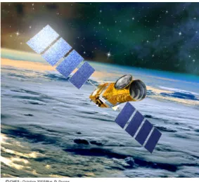
1.4 CoRoT . . . . 31
1.5 Overview of exoplanet properties . . . . 37
2 Theory of tidal interaction 41 2.1 The gravitational potential . . . . 42
2.1.1 The outer gravitational potential . . . . 42
2.1.2 Inner gravity potential . . . . 45
2.2 The role of Legendre polynomials in axial symmetric gravity potentials 46 2.2.1 Potential theory . . . . 48
2.3 Tidal force and potential . . . . 51
2.4 Deformation of celestial bodies . . . . 57
2.4.1 Tidal deformation . . . . 57 iii
2.7 Tidal evolution of eccentric orbits . . . . 80
2.8 The tidal dissipation factor and the Love number . . . . 89
2.8.1 Q/k2 in the Solar System . . . . 90
2.8.2 Q/k2 in extrasolar planet systems . . . . 94
2.9 Stability of tidal equilibrium . . . . 98
2.10 Evolution of the rotation of main sequence stars . . . . 105
2.11 Moment of Inertia . . . . 113
2.12 The Roche limit . . . . 115
3 Critical examination of assumptions and approximations 119 3.1 The constant Q∗-assumption . . . . 119
3.1.1 Can Q∗ be regarded as constant even though the system may meet resonant states? . . . . 120
3.1.2 Can Q∗ be regarded as constant although it is defined as fre- quency dependent? . . . . 121
3.1.3 What happens with Q∗ when the system approaches double synchronicity? . . . . 122
3.1.4 Switching from the constant Q- to the constant τ-formalism. . 124
3.2 Is the planetary rotation tidally locked? . . . . 126
3.3 Energy and angular momentum in close-in extrasolar planetary systems 131 3.3.1 Possible pitfalls in the calculation of the Roche zone . . . . 133
4 Close-in extrasolar planets as playground for tidal friction models 136 4.1 The tidal stability maps for planets around main sequence stars . . . 136
4.1.1 CoRoT systems most strongly affected by tidal friction . . . . 144
5 Constraining kQ∗ 2,∗ by requiring orbital stability of close-in planets around slowly rotating stars 149 5.1 Tidal evolution of the semi major axis of CoRoT-Planets on circular orbits . . . . 150
5.1.1 Tidal evolution of the semi major axis of CoRoT-Planets on circular orbits around low mass stars . . . . 151
5.1.2 Tidal evolution of the semi major axis of planets on circular orbits around F stars and subgiants . . . . 156
5.2 Tidal evolution of the semi major axis and eccentricity of planets on eccentric orbits . . . . 158
iv
e >0.5 . . . . 174
5.2.3 Orbital stability for planets on eccentric orbits . . . . 175
5.3 Limits of stability on potentially unstable systems . . . . 177
6 Constraining kQ∗ 2,∗ by stellar rotation evolution of slowly rotating stars178 6.1 Tidal rotation evolution of the host stars of CoRoT-Planets on circular orbits . . . . 179
6.1.1 Tidal rotation evolution of low mass host stars of CoRoT-Planets on circular orbits . . . . 180
6.1.2 Tidal rotation evolution of F-spectral type host stars of CoRoT- Planets on circular orbits . . . . 183
6.2 Tidal rotation evolution of host stars of CoRoT-Planets on eccentric orbits . . . . 190
6.2.1 How does the stellar rotation evolution change with larger kQP l 2,P l 194 6.2.2 Positive feedback effect for planets on orbits with e >0.5 . . . . 194
6.3 Using stellar rotation as a ’smoking gun’ for the influence of tidal friction198 6.4 Evaluating evidence for tidal spin up . . . . 203
6.5 A word regarding the evolution of the tidal frequencies . . . . 204
7 Tidal evolution of close-in exoplanets around fast rotating stars 205 7.1 The tidal evolution of the CoRoT-6 system . . . . 210
7.2 The tidal evolution of the CoRoT-11 system . . . . 212
7.3 Orbital stability . . . . 216
7.4 Results of the stellar rotation evolution . . . . 216
8 Double synchronous states 219 8.1 The stability of the double synchronous CoRoT systems . . . . 219
8.2 Constraints on kQ∗ 2,∗ to achieve a double synchronous state in the pres- ence of magnetic braking . . . . 224
8.3 Long-term stability of double synchronous orbits in the presence of magnetic braking . . . . 233
8.3.1 The possible decay of the double synchronous orbit due to mag- netic braking . . . . 236
8.4 Tidal evolution of the CoRoT-3 and CoRoT-15 system . . . . 240
v
k2,∗
tation state . . . . 259
9 Summary and Discussion 263 Appendix 273 A CoRoT planet references 274 B Tidal evolution of CoRoT-4 and CoRoT-9 276 C |Ω∗−n| evolution for close-in CoRoT-planets 279 D Evolution of the rotation of CoRoT planets on eccentric orbits 289 E Integration method 293 F Model sensitivity analysis 299 F.1 The CoRoT-12 system . . . . 300
F.2 The CoRoT-16 system . . . . 302
F.3 The CoRoT-20 system . . . . 304
F.4 The CoRoT-11 system . . . . 308
F.5 The CoRoT-15 system . . . . 308 G Proof that the double synchronous orbit is always forced into cor-
rotation if Lorb > Lorb,crit 313
H Centrifugal versus gravitational force 315
Acknowledgements 339
Erkl¨arung 340
Lebenslauf 341
vi
1.1 Planet types discovered by the CoRoT space mission. . . . 32 1.2 Stellar parameters of CoRoT-1 to -21. . . . 34 1.3 Planetary parameters of CoRoT-1b to -21b. . . . . 35 1.4 Stellar rotation period of CoRoT-1 to -21 and planetary revolution of
CoRoT-1b to -21b. . . . 36 2.1 Normalized moment of inertia for some ideal bodies . . . . 114 2.2 Normalized moment of inertia for some solar system bodies . . . . 114 3.1 Synchronization time scale τsynchr for the CoRoT-planets. A slow ro-
tator is a planet with an initial rotation period PP l = 10 days, a fast rotator is a planet with an initial rotation period ofPP l= 10 hours. . 128 3.2 Comparison of Roche limit approximations . . . . 135 4.1 The parameters of the central stars used for the calculation of the tidal
stability maps. Real stars were selected as representatives of K-, G- and F-spectral type stars, respectively. . . . 138 4.2 The parameters of the exoplanets placed around each star (Table 4.1)
for the calculation of the tidal stability map. A real planet was selected as a representative for each exoplanet category. . . . . 139 5.1 Required kQ∗
2,∗stable for the planet’s orbit to stay outside the Roche limit within the minimum, average, and maximum remaining lifetime of the star. . . . 155
vii
5.3 Equivalent semi major axisaequiv(equation 5.2.8) of the CoRoT-planets on eccentric orbits. . . . 173 5.4 Required kQ∗
2,∗stable for the planet’s orbit to stay outside the Roche limit within the minimum, average and maximum remaining lifetime of the star. . . . 176 6.1 Required kQ∗
2,∗ for tidal friction to compensate magnetic braking at the planet’s current position. . . . 199 6.2 Required kQ∗
2,∗ for tidal friction to compensate magnetic braking for planets on eccentric orbits at the current position. . . . 202 7.1 Required kQ∗
2,∗stable for the planet’s orbit to stay outside the Roche limit within the remaining lifetime of the star. . . . 217 8.1 Required kQ∗
2,∗ for tidal friction to compensate magnetic braking at the planet’s current position. . . . 259 8.2 Required kQ∗
2,∗ for tidal friction to allow for minimal migration in the past.261 A.1 References for the parameters of the CoRoT planetary systems. . . . 275
viii
1.1 Histogram of the masses of all detected exoplanets. The data were taken from the exoplanet catalogue: http://www.exoplanet.eu/catalog- all.php as of 14th October 2011. . . . . 12 1.2 The motion of a star and a planet with massesM∗ and MP l and semi
major axes a∗ and aP l, respectively, around their common center of mass (CM). . . . 16 1.3 The orbital plane of a planetary system which is inclined by the angle
i with respect to the line-of-sight. The system consists of a star and a planet with masses M∗ and MP l, revolving with semi major axes a∗ and aP l, respectively, around their common center of mass. . . . 17 1.4 As the star moves around the barycenter, emitted light is Doppler
shifted (Credit: ESO). . . . 19 1.5 Radial velocity curve of 51 Pegasi b. The planet induces a radial
velocity modulation of about 50 m/s (Mayor and Queloz, 1995). . . . 21 1.6 Left panel: Schema of the microlensing effect (Credit: OGLE).
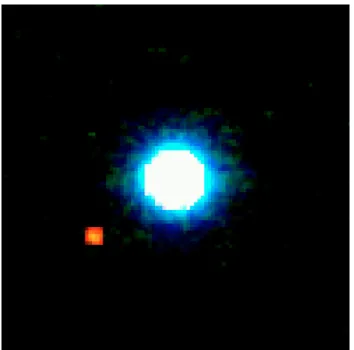
Right panel: Photometric curve with best-fitting double-lens models of OGLE 2003-BLG-235/MOA 2003-BLG-53 b (Bond et al., 2004). . 25 1.7 Composite image of the brown dwarf 2M1207 and its gas giant com-
panion in the infrared (Chauvin et al., 2004). . . . 27 1.8 As the planet passes in front of its star, the apparent brightness of the
star decreases by ∆F (Credit: Hans Deeg, ESA). . . . . 28 1.9 Probability to observe a transit from Earth. . . . 29
ix
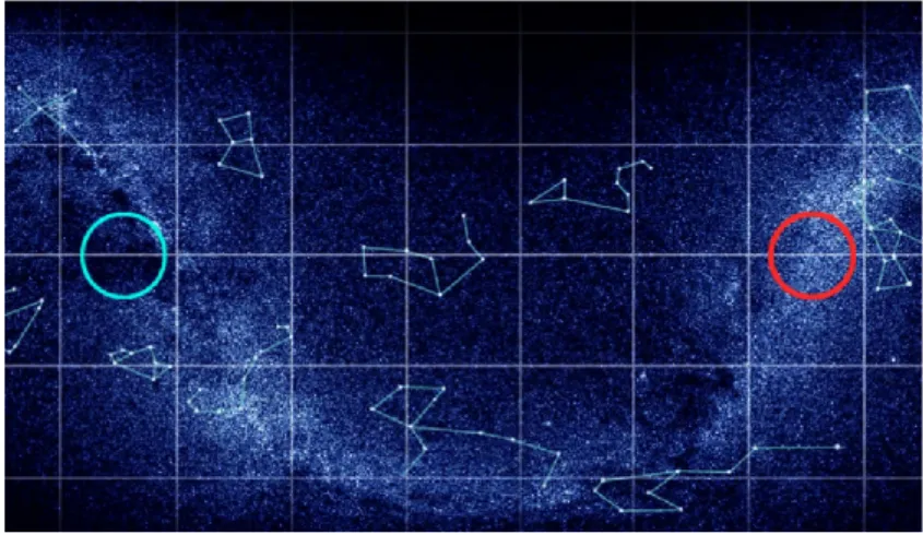
1.11 The CoRoT ’eyes’ in the night sky (diameter:10◦). The ’red’ circle is observed in summer and contains the Aquila constellation. The ’blue’
circle is observed in winter and lies in the Monoceros constellation (CNES). . . . 32 1.12 Histogram of the masses of all detected exoplanets in logarithmic scale. 37 1.13 Left panel: Histogram of the semi major axis of all detected exoplanets.
Right panel: Histogram of the semi major axis of exoplanets in close proximity to their star in units of solar radii. . . . 38 1.14 Left panel: Histogram of the masses of all detected transiting exoplan-
ets. Right panel: Histogram of the masses of all detected transiting exoplanets in logarithmic scale. . . . 39 1.15 Left panel: Histogram of the semi major axis of all detected transiting
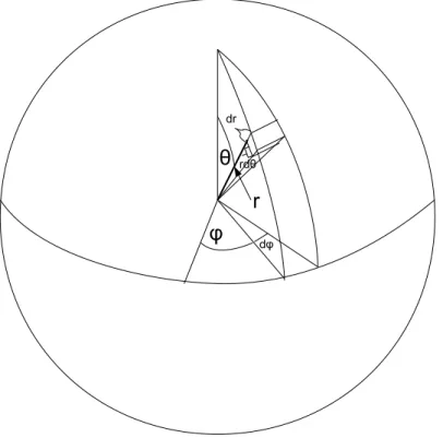
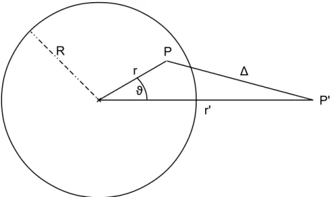
exoplanets. Right panel: Histogram of the semi major axis of transiting exoplanets in units of solar radii. . . . . 40 2.1 The parameters of the mass element dm in polar coordinates. . . . . 43 2.2 The distance ∆ betweenP, the position of the mass element dm, and
the reference pointP′ in polar coordinates . . . . 44 2.3 The potential of mass element at Pi as seen from an outer reference
point P′ in a spherical coordinate system. . . . . 47 2.4 The location of two points P and P′ on a unit sphere. . . . 50 2.5 The relationships between the radius of the primary,RP, the radius of
the orbit of the secondary, a, and the distance ∆ from a point P on the surface of the primary to the center of mass of the secondary. . . 52 2.6 Centrifugal versus gravitational force at different points within the pri-
mary. . . . 54
x
gravityCM. This is illustrated by the movement ofP′ about the point CM′ and the center of the primary CP about CM. In this picture the rotation of the primary about its polar axis is neglected. . . . . 55 2.8 The deformation of a homogenous sphere due to the tidal potential. . 58 2.9 The tidal deformation of a two-component model planet of radius
Rmean and density ρo and a core of radiusRCore and density ρc. . . . 61 2.10 Centrifugal force in a primary rotating about its polar axis with the
rotation rate Ω in a coordinate system where the angle θ is measured from the rotation axis. . . . 65 2.11 Left: Symmetry axis with respect to the tidal deformation.
Right: Symmetry axis with respect to the rotation of the body. . . . 69 2.12 Upper panel: If the primary’s rotation is faster than the secondary’s
revolution (ΩP > n), the tidal bulge is carried ahead the line con- necting the two center of masses. The tidal torques decrease ΩP and increasen.
Middle panel: If the primary’s rotation is slower than the secondary’s revolution (ΩP < n), the tidal bulge is lagging behind the line con- necting the two center of masses. The tidal torques increase ΩP and decreasen.
Lower panel: If the system is in retrograde revolution, the tidal torques decrease ΩP and n. . . . . 77 2.13 The barycentric orbit configuration of a binary system including its
relevant parameters. L⃗ is the total angular momentum L⃗tot and ⃗h is the orbital angular momentumL⃗orb (Hut, 1980). . . . 99
xi
ncrit, two double synchronous states exist. Arrows show the direction of decreasing total energy. The stability of a given double synchronous state is determined by the total energy: Stability is only ensured if the total energy is minimal as well. For n = ncrit only one solution with Ltot,doub = Lcrit exists. For Ltot,doub < Lcrit, no double synchronous state can be achieved. . . . . 104 2.15 Evolution of the stellar radius, radius of gyrationI(=moment of inertia
C∗ in the notation used in this work) for 0.5,0.8 and 1MSun stars (Bouvier et al., 1997). . . . . 106 2.16 Ca+emission luminosity, rotation velocity and lithium abundance with
age. Shown as an example are the properties of stars in the Pleidaes (0.04 Gyrs), Ursa Major (0.15 Gyrs), the Hyades Cluster (0.4 Gyrs) and the Sun (4.5 Gyrs). In 1972 the age estimate of the Hyades Cluster was controversial. Other age estimates would have resulted in a shift of the Pleiades data points along the x-axis as indicated by the arrows (Skumanich, 1972). . . . 109 2.17 Color-period diagrams (B−V versus rotation period, on a linear scale)
for a series of open clusters and Mount Wilson stars with different ages.
Note the change in scale for the old Mount Wilson stars. The higher B−V, the redder the star, the less hot the stellar surface and the lower the mass of the star. On the other hand, the smaller B−V, the bluer the star, the hotter the stellar surface, the higher the mass of the star (Barnes, 2003). . . . 112 2.18 The solar seismic model taken from Dziembowski et al.(1994). r is the
radius from the center of the Sun, u is the square of isothermal speed of sound at radiusr,ρ is the density at radiusr,P is the pressure and M(r) is the integrated mass up to r. . . . . 115
xii
Right panel: Planetary revolution rate versus semi major axis of a close-in extrasolar Jupiter analogue around a Sun-like star. . . . 121 3.2 Synchronization time scalesτsynchr and the age of the CoRoT planets
versus their semi major axes. The black solid lines represent τsynchr calculated for a slow (10 days) and a fast (10 hours) primordial plan- etary rotation. The grey lines represent the system ages within the limit of uncertainties. The age of CoRoT-9b, a planet orbiting its star beyond 0.4 AU, is represented by a dotted grey line. In this case, the system age and the possible synchronization time scale overlap each other. . . . . 129 3.3 Relative brightness in the infrared estimated for 12 longitudinal strips
on the surface of the planet HD 189733. Data are shown as a colour map (a) and in graphical form (b) (Knutson et al., 2007). . . . 130 3.4 Density of transiting exoplanets versus their mass. . . . 134 4.1 Tidal stability maps for different exoplanets around a K-star. From
top to bottom, from left to right: A high mass brown dwarf, a low mass brown dwarf, a hot Jupiter, a Neptune, a Super-Earth, an Earth and a Mercury planet. The grey color gives the time scale τRoche in log(109 years). The total lifetime of the star is indicated as a white dashed line. The black lines are the isochrones ofτRoche. The horizontal and vertical dashed white lines indicate the stability limitathreshold for every kQ∗
2,∗. . . . 141 4.2 Tidal stability maps for different exoplanets around a G-star. See also
Figure 4.1. . . . 142 4.3 Tidal stability maps for different exoplanets around an F-star. See also
Figure 4.1. . . . 143
xiii
for tides raised by the Earth on the Moon, E denotes the Doodson constant for lunar tides raised on Earth, J denotes tides raised by Jupiter on the Sun and Me denotes the Doodson constant for tides raised by Mercury on the Sun. . . . 145 4.5 The tidal property factor for tides raised by the planets CoRoT-1b to
CoRoT-21b on their stars. . . . 146 5.1 The tidal evolution of the semi major axis of the planets CoRoT-1b,
-2b, -7b, -8b, -12b, -13b, -17b and -18b for the next 1.5×10¹⁰years and for kQ∗
2,∗ = 105−109. The horizontal lines mark Roche limits (from top to bottom: aRoche,hydro, aRoche,inter, aRoche,rigid) which span the Roche zone (Section 2.12). At the distance a = 1R∗, another horizontal line marks the stellar surface. The vertical grey lines show the remaining lifetime of the system. The solid vertical line is the total lifetime of the star computed by 4.1.2 minus the age of the system. The dotted vertical lines are the minimum and maximum remaining lifetime of the system (lifetime−age±∆age). For CoRoT-1, no age is known. A black vertical line marks the total lifetime. CoRoT-17 has reached the end of its lifetime, this is indicated by a black vertical line at the start point of the evolution. . . . 152 5.2 The tidal evolution of the semi major axis of the planets CoRoT-5b,
14b, 19b, and -21b for the next 1.5×10¹⁰years and for kQ∗
2,∗ = 105−109. The horizontal lines span the Roche zone. The horizontal line at a = 1R∗ marks the stellar surface. The vertical lines show the remaining lifetime of the system. See Figure 5.1 for a more detailed description. 156
xiv
105,106,107,108,109 and kQP l
2,P l = 104. The horizontal lines span the Roche zone. The horizontal line at a = 1R∗ marks the stellar sur- face. The vertical lines show the remaining lifetime of the system. See Figure 5.1 for a more detailed description. . . . 162 5.4 The tidal evolution of the orbit eccentricity of CoRoT-10b, -16b, and
CoRoT-20b for the next 1.5×10¹⁰ years, for kQ∗
2,∗ = 105 −109 (solid lines) and kQP l
2,P l = 104. The vertical lines show the remaining lifetime of the system. . . . 164 5.5 Close-up of the orbit eccentricity evolution of CoRoT-10b and -16b due
to tides for kQ∗
2,∗ = 105−109 and kQP l
2,P l = 104. . . . . 165 5.6 The tidal evolution of the semi major axis of the planets CoRoT-10b
for the next 1.5×10¹⁰ years in more detail, for kQ∗
2,∗ = 105 −109 and
QP l
k2,P l = 104. The vertical lines show the remaining lifetime of the system.166 5.7 The tidal evolution of the semi major axis of CoRoT-10b, -16b, and
CoRoT-20b for the next 1.5× 10¹⁰ years, for kQ∗
2,∗ = 105 −109 and
QP l
k2,P l = 105. The horizontal lines span the Roche zone. The horizontal line at a = 1R∗ marks the stellar surface. The vertical lines show the remaining lifetime of the system. See Figure 5.1 for a more detailed description. . . . 168 5.8 The tidal evolution of the orbit eccentricity of CoRoT-10b, -16b, and
CoRoT-20b for the next 1.5×10¹⁰ years, for kQ∗
2,∗ = 105 −109 (solid lines) and kQP l
2,P l = 105. The vertical lines show the remaining lifetime of the system. . . . 169
xv
QP l
k2,P l = 106. The horizontal lines span the Roche zone. The horizontal line at a = 1R∗ marks the stellar surface. The vertical lines show the remaining lifetime of the system. See Figure 5.1 for a more detailed description. . . . 170 5.10 The tidal evolution of the orbit eccentricity of CoRoT-10b, -16b, and
CoRoT-20b for the next 1.5×10¹⁰ years, for kQ∗
2,∗ = 105 −109 (solid lines) and kQP l
2,P l = 106. The vertical lines show the remaining lifetime of the system. . . . 171 6.1 The tidal evolution of the stellar rotation of CoRoT-1, -2, -7, -8, -12, -
13, -17 and -18 for the next 1.5×10¹⁰years and for kQ∗
2,∗ = 105−109(solid lines). The dashed-dotted lines show the evolution of the orbital period of the corresponding close-in planet for comparison. The vertical lines show again (like in Figure 5.1) the remaining lifetime of the system. . 181 6.2 The tidal evolution of the stellar rotation of CoRoT-5, -14, 19, and -21
for the next 1.5×10¹⁰ years and for kQ∗
2,∗ = 105−109 (solid lines) in the presence of full magnetic braking. The dashed-dotted lines show the evolution of the orbital period of the corresponding close-in planet for comparison. The vertical lines show the remaining lifetime of the system. . . . 185 6.3 The tidal evolution of the stellar rotation of CoRoT-5, 14, 19, and -21
for the next 1.5×10¹⁰ years and for kQ∗
2,∗ = 105−109 (solid lines) in the presence of reduced magnetic braking. . . . . 186 6.4 The tidal evolution of the stellar rotation of CoRoT-5, 14, 19, and -
21 for the next 1.5×10¹⁰ years and for kQ∗
2,∗ = 105−109 (solid lines) without magnetic braking. . . . 187
xvi
lines) and kQP l
2,P l = 104. The dashed-dotted lines show the evolution of the orbital period of the corresponding close-in planet for comparison.
The vertical lines show the remaining lifetime of the system. . . . 192 6.6 The tidal evolution of the stellar rotation of CoRoT-9,-10, -16, and
CoRoT-20 for the next 1.5×10¹⁰ years, for kQ∗
2,∗ = 105 − 109 (solid lines) and kQP l
2,P l = 105. The dashed-dotted lines show the evolution of the orbital period of the corresponding close-in planet for comparison.
The vertical lines show the remaining lifetime of the system. . . . 195 6.7 The tidal evolution of the stellar rotation of CoRoT-9,-10, -16, and
CoRoT-20 for the next 1.5×10¹⁰ years, for kQ∗
2,∗ = 105 − 109 (solid lines) and kQP l
2,P l = 106. The dashed-dotted lines show the evolution of the orbital period of the corresponding close-in planet for comparison.
The vertical lines show the remaining lifetime of the system. . . . 196 6.8 The stellar rotation periods of the CoRoT-stars of spectral type K and
G versus age including the limits of uncertainties. The stellar rotation of CoRoT-17 stands out because it is faster than expected for such an old star. . . . 200 6.9 The stellar rotation periods of the spectral type F CoRoT-stars versus
age including the limits of uncertainties. The blue crosses are the rotation periods and the age of CoRoT-3 and CoRoT-15. . . . 201 7.1 The tidal evolution of the semi major axis of the planets CoRoT-6b,
and -11b for the next 1.5×10¹⁰ years and for kQ∗
2,∗ = 105−109. The horizontal lines span the Roche zone. The horizontal line at a = 1R∗ marks the stellar surface. The vertical lines show the remaining lifetime of the system. See Figure 5.1 for a more detailed description). . . . . 208
xvii
reduced and without magnetic braking. The dashed-dotted lines show the evolution of the orbital period of the corresponding close-in planet for comparison. The vertical lines show the remaining lifetime of the system. . . . 209 7.3 The tidal evolution of the semi major axis of the planets CoRoT-6b
for the next 1.5×10¹⁰ years and for kQ∗
2,∗ = 105−109. They-axis is this time set to linear scale and spans from 0.04 to 0.1 AU. . . . 210 7.4 The tidal evolution of the stellar rotation of CoRoT-11 with reduced
magnetic braking for the next three billion years and for kQ∗
2,∗ = 105 and 106. . . . 214 8.1 Comparison of the total angular momentum,Ltot, of the CoRoT plan-
ets with the critical angular momentum,Ltot,crit, and comparison of the orbital angular momentum of the CoRoT systems,Lorb, with the crit- ical orbital angular momentum Lorb. Top: The ratio Ltot over Ltot,crit
for each CoRoT system. Bottom: The ratio of Lorb and Lorb,crit for each CoRoT system. . . . 221 8.2 The orbit of a planet around a star with respect to the double syn-
chronous orbit (n = Ω∗, solid line). If n < Ω∗, the orbit lies outside the double synchronous orbit (dashed line). If n > Ω∗, the orbit lies inside the double synchronous orbit (dotted line) . . . . 227 8.3 Evolution of the subsynchronous orbit n0 > Ω∗,0 represented by the
dotted blue circle with respect to the double synchronous orbit repre- sented by the solid blue circle into a double synchronous orbitn1 = Ω∗,1 represented by the red solid circle. . . . 229
xviii
by the solid blue circle if magnetic braking is more efficient than tidal friction. In the next time step, the planet’s orbit would shrink (dot- ted red circle) but the stellar rotation would decrease and lead to a double synchronous orbit with even larger radius, where n1 = Ω∗,1, represented by the red solid circle. . . . 231 8.5 Evolution of double synchronous orbit n1 = Ω∗,1 represented by the
solid blue circle in the presence of magnetic braking. The stellar rota- tion becomes slower and as a consequence the radius of the new double synchronous orbit is larger than the radius of the previous one (solid red circle), while the planet’s orbit (dotted red circle) remains at its position. This is the same situation than depicted in Figure 8.3. . . . 234 8.6 The decay of a double synchronous orbit (red circles) in the presence
of magnetic braking starting with a subsynchronous planetary orbit (the blue dotted circle is the planet’s orbit, the blue solid line is the
’fictive’ double synchronous orbit that lies outside the planet’s orbit).
In the first step, the planetary and double synchronous orbit converge to a new double synchronous orbit with smaller radius(red). In the next step, the stellar rotation decreases and for this state the ’fictive’
double synchronous orbit (blue) would lie outside the ’old’ double syn- chronous state where the planet is still orbiting the star. In the next step, the planet’s and double synchronous orbit converge into a new double synchronous orbit with even smaller radius etc. In consequence, the planetary orbit continually shrinks. The double synchronous orbit alternatively shrinks and expands, as indicated by the black arrows. . 237
xix
horizontal lines span the Roche zone. The horizontal line at a = 1R∗ marks the stellar surface. The vertical lines show the remaining lifetime of the system. . . . 241 8.8 The tidal evolution of the stellar rotation of CoRoT-3, and -15 for the
next 1.5×10¹⁰ years and for kQ∗
2,∗ = 105 −109 (solid lines) with full, reduced and without magnetic braking. The dashed-dotted lines show the evolution of the orbital period of the corresponding close-in planet for comparison. The vertical lines show the remaining lifetime of the system. . . . 242 8.9 Close-up of the tidal evolution of the semi major axis of the Brown
Dwarfs CoRoT-3b, and -15b for the next one billion years and for
Q∗
k2,∗ = 105 −109. . . . 243 8.10 Close-up of the tidal evolution of the stellar rotation of CoRoT-3, and
-15 for the next one billion years and for kQ∗
2,∗ = 105−109 (solid lines) with full, reduced and without magnetic braking. The dashed-dotted lines show the evolution of the orbital period of the corresponding close-in planet for comparison. . . . . 244 8.11 Close-up of the tidal evolution of the semi major axis of the Brown
Dwarfs CoRoT-3b for the next 15 billion years and kQ∗
2,∗ = 105 −109. Vertical lines denote the minimum, average and maximum remaining lifetime. . . . 247 8.12 The evolution of the ratio of total angular momentumLtot over critical
total angular momentumLtot,crit for the CoRoT-20 system under tidal friction and magnetic braking with kQP l
2,P l = 105 and kQ∗
2,∗ = 106. The horizontal dashed line marksLcrit,tot. . . . 252
xx
semi major axis, the eccentricity, the stellar rotation (solid lines) and planetary orbital revolution period (dashed lines), and of|Ω∗−n| for
Q∗
k2,∗ = 105−109 and kQP l
2,P l = 104. The vertical lines show the remaining stellar lifetime with limits of uncertainty. . . . 253 8.14 Tidal evolution of the CoRoT-20 system with P∗ = 8.9 days as initial
condition of the stellar rotation. The panels show the evolution of the semi major axis, the eccentricity, the stellar rotation (solid lines) and planetary orbital revolution period (dashed lines), and of|Ω∗−n| for
Q∗
k2,∗ = 105−109 and kQP l
2,P l = 105. The vertical lines show the remaining stellar lifetime with limits of uncertainty. . . . 254 8.15 Tidal evolution of the CoRoT-20 system with P∗ = 8.9 days as initial
condition of the stellar rotation. The panels show the evolution of the semi major axis, the eccentricity, the stellar rotation (solid lines) and planetary orbital revolution period (dashed lines), and of|Ω∗−n| for
Q∗
k2,∗ = 105−109 and kQP l
2,P l = 106. The vertical lines show the remaining stellar lifetime with limits of uncertainty. . . . 255 8.16 Tidal evolution of the CoRoT-20 system with P∗ = 8.9 days as initial
condition of the stellar rotation focusing on the first one billion years evolution time. The panels show the evolution of the semi major axis, the eccentricity, the stellar rotation (solid lines) and planetary orbital revolution period (dashed lines), and of |Ω∗−n| for kQ∗
2,∗ = 105 −109 and kQP l
2,P l = 105. . . . 257 B.1 Tidal evolution of the of the CoRoT-4 system for for kQ∗
2,∗ = 105−109,
QP l
k2,P l = 105, and full, reduced and without magnetic braking. The
vertical lines show the remaining stellar lifetime with limits of uncertainty.277
xxi