Effects of Securities Transaction Taxes on Depth and Bid-Ask Spread

IHS Economics Series Working Paper 132

May 2003

Effects of Securities Transaction Taxes on Depth and Bid-Ask Spread

Dominique Y. Dupont

Gabriel S. Lee

Impressum Author(s):

Dominique Y. Dupont, Gabriel S. Lee Title:

Effects of Securities Transaction Taxes on Depth and Bid-Ask Spread ISSN: Unspecified

2003 Institut für Höhere Studien - Institute for Advanced Studies (IHS) Josefstädter Straße 39, A-1080 Wien

E-Mail: o ce@ihs.ac.atffi Web: ww w .ihs.ac. a t

All IHS Working Papers are available online: http://irihs. ihs. ac.at/view/ihs_series/

This paper is available for download without charge at:

https://irihs.ihs.ac.at/id/eprint/1493/

132 Reihe Ökonomie Economics Series

Effects of Securities Transaction Taxes on Depth and Bid-Ask Spread

Dominique Y. Dupont, Gabriel S. Lee

132 Reihe Ökonomie Economics Series

Effects of Securities Transaction Taxes on Depth and Bid-Ask Spread

Dominique Y. Dupont, Gabriel S. Lee May 2003

Institut für Höhere Studien (IHS), Wien

Institute for Advanced Studies, Vienna

Contact:

Dominique Y. Dupont University of Twente

School of Management and Technology Department of Finance and Accounting Postbus 217

7500 AE Enschede, The Netherlands : +31/53/489 44 70

fax: +31/53/489 21 59 email: d.dupont@sms.utwente.nl Gabriel S. Lee

Department of Economics and Finance Institute for Advanced Studies Stumpergasse 56

1060 Vienna, Austria : +43/1/599 91–141 fax: +43/1/599 91–555 email: gabriel.lee@ihs.ac.at

Founded in 1963 by two prominent Austrians living in exile – the sociologist Paul F. Lazarsfeld and the economist Oskar Morgenstern – with the financial support from the Ford Foundation, the Austrian Federal Ministry of Education and the City of Vienna, the Institute for Advanced Studies (IHS) is the first institution for postgraduate education and research in economics and the social sciences in Austria.

The Economics Series presents research done at the Department of Economics and Finance and aims to share “work in progress” in a timely way before formal publication. As usual, authors bear full responsibility for the content of their contributions.

Das Institut für Höhere Studien (IHS) wurde im Jahr 1963 von zwei prominenten Exilösterreichern – dem Soziologen Paul F. Lazarsfeld und dem Ökonomen Oskar Morgenstern – mit Hilfe der Ford- Stiftung, des Österreichischen Bundesministeriums für Unterricht und der Stadt Wien gegründet und ist somit die erste nachuniversitäre Lehr- und Forschungsstätte für die Sozial- und Wirtschafts- wissenschaften in Österreich. Die Reihe Ökonomie bietet Einblick in die Forschungsarbeit der Abteilung für Ökonomie und Finanzwirtschaft und verfolgt das Ziel, abteilungsinterne Diskussionsbeiträge einer breiteren fachinternen Öffentlichkeit zugänglich zu machen. Die inhaltliche Verantwortung für die veröffentlichten Beiträge liegt bei den Autoren und Autorinnen.

Abstract

This paper investigates the effects of transaction taxes on depth and bid-ask spread under asymmetric information. The paper uses a static model where a monopolistic market maker faces liquidity and informed traders. Introducing transaction taxes could, surprisingly, lead to increase in depth. Under some distributional assumptions, when market conditions are favorable to the dealer, the spread responds less than proportionally to an increase in the transaction tax while the depth actually increases. In contrast, when market conditions are unfavorable to the dealer, the spread widens more than proportionally and the depth decreases, potentially to zero, in response to an increase in the transaction tax. Our model sheds light on the disagreement in the empirical literature on the relative magnitude of transaction costs on trading volume.

Keywords

Asymmetric information, securities transaction taxes, liquidity

JEL Classifications

G14, D82

Comments

We thank Vincent Reinhart, Walter Fisher and seminar participant at the Institute for Advanced Studies, Vienna for helpful discussions. This paper was partially written when Dominique Dupont was at the Board of Governors of the Federal Reserve System.

Contents

1. Introduction 1

2. Model 3

3. Equilibrium with discrete distributions 5 4. Equilibrium with continuous distributions 8

4.1. Marginal condition ... 8 4.2. Expected dealer's profit ... 10 4.3. Numerical results ... 11

5. Conclusion 15

References 16

1. Introduction

This paper investigates the effects of securities transaction taxes (STT) on the liquidity of a quote-driven market under asymmetric information. Academics and

Þnancial market regulators

(e.g. Dow and Rahi (2000, OECD (2002), and Hakkio (1994)) have studied the potential effects of imposing securities transaction taxes (akin to the Tobin tax) as an instrument to curb speculation and excess volatility without impairing market liquidity. Kyle (1985) states that liquidity can be measured by bid-ask spread, depth and resiliency.

¹

Past research, however, uses an aggregate measure of liquidity, trading volume, in analysing the relationship between transaction costs and liquidity. In this paper, we examine the effects of taxation on a disaggregate level using bid-ask spread and depth.

²

Consequently, our results can accommodate some of the disagreements in the empirical literature on the relative magnitude of transaction taxes on trading volume (Kandel and Marx (1998) and Brennen, Chordia and Subrahmanyam (1998)).

Our model builds on Glosten and Milgrom (1985), who study the pricing strategy of an uninformed market maker facing potentially better informed traders. Our approach, however, differs from Glosten and Milgrom (1985) in the following way. First, they assume the existence of an equilibrium whereas we characterize the conditions for the existence of an equilibrium in our framework. Moreover, as in Dupont (2000), we incorporate both spread and depth into a model that allows the theoretical dealer to adjust the depth differently than the bid-ask spread in response to changes in the degree of information asymmetry. In this setting, we analyze the effects of transaction tax on market liquidity across different levels of information asymmetry.

1Resiliency is the speed with which priceßuctuations resulting from trades are dissipated, and depth is the maximum amount the dealer stands ready to sell or buy at the posted prices. See Kyle (1985) for details.

2Previous research on the relationship between transaction costs and trading volume can be used to study the effects of transaction taxes on liquidity (see among many, Constantinides (1986), Barclay, Kandel and Marx (1998), Vayanos (1998), and Vayanos andVila (1999)).

1

Our analysis uses a one-period model where a monopolistic market maker posts

Þrm prices

(including tax) and depths on the bid and ask sides, while facing a risk-neutral informed trader and a liquidity trader. The informed trader observes a private signal correlated with the true value of the asset. The demand of the liquidity trader is price sensitive and subject to the liquidity shock.

Our results can be summarized as follows. First, introducing a transaction tax could lead to either increase or decrease in depth, depending on the degree of information asymmetry and liquidity demand. Secondly, the spread could respond disproportionally to increase in tax.

Subsequently, our results seem to point to two regimes as far as transaction tax is concerned.

First, when information asymmetry is weak or liquidity demand is strong (i.e., when market conditions are favorable to the market maker), the market maker pays part of the transaction tax himself by increasing the spread less than the tax. Moreover, he quotes a larger depth to attract order

ßow in order to make up for the loss in demand due to the transaction tax. On

the other hand, when market conditions are unfavorable, increasing the transaction tax leads to a drastic reduction in the liquidity provided by the market maker, enticing him to exit the market. In turn, the paper suggests that lowering transaction tax may not necessarily lead to increase in quoted depth.

Our paper is structured as follows. The next section introduces the model. To numerically analyze our model under various distributional assumptions, we study two cases. Section 3 analyses the equilibrium conditions under a discrete distribution: the asset value, the informed trader’s signal and the liquidity shock each take two values. Section 4 looks at the equilibrium conditions under continuous distributions where the asset value is lognormally distributed with mean 1. Both the private signal and the liquidity shock are, however, normally distributed.

2

Section 5 concludes the paper.

2. Model

A monopolistic dealer posts

Þrm prices and depths on the bid and ask sides. He faces a price-

sensitive liquidity trader and a trader possessing private information about the value of the asset. The liquidity trader’s demand is price sensitive and stochastic. The informed trader, who observes a signal correlated with the true value of the asset, buys the asset if the ask is below (or sells if the bid is above) his valuation. For simplicity, we assume no limit-order book or

ßoor

brokers compete with the dealer (or specialist). The model focuses on asymmetric information and excludes other factors such as misdiversiÞcation and order-processing costs.

To simplify computations, we assume that the informed trader is risk neutral. His demand is satisÞed before that of the liquidity trader. This assumption simpliÞes the informed trader’s demand but excludes some strategies potentially available to actual traders, such as conditioning orders on the volume of liquidity trade. Informed and liquidity traders’ buy or sell orders are lumped together and passed on to the dealer so that the quantity limit becomes binding if the sum of all orders is greater than the posted depth.

We study only the ask side of the dealer’s activity as the bid side is symmetrical. Let x be the true value of the asset, c the transaction tax, a the ask price inclusive of tax, z the quantity limit, G the informed trader’s private signal, v = E[x|G] his valuation of the traded asset,

η

the liquidity shock (η and G are independently distributed), and d(a) the liquidity trader’s demand.

The orders of the liquidity trader and of the informed trader are pooled together and passed on to the dealer. By convention, the dealer pays the transaction tax but, ceteris paribus, the

3

transaction tax could be levied on the customers. To acquire one unit of the traded asset, informed and liquidity traders pay a but the dealer receives only (a

−

c) if the transaction tax is a

Þxed amount per transaction (Þxed transaction tax), or

(

_1+c^a

) if it is a

Þxed percentage of

the price (proportional transaction tax).

The effective demand, S(a, z, v,

η),

depends on the realization of liquidity shocks and the valuation of informed trader. If v > a, then a risk neutral informed trader will demand the maximum amount.

³

On the other hand, if v

·

a then the informed trader does not participate and hence the transaction volume on the ask side depends on the liquidity demand. The following equation represents the effective demand:

S(a, z, v,

η) =

I(v

·

a) I(d(a)

≥

0) min(d(a), z) + I(v > a) z (2.1)

where I the indicator function. Consequently, the dealer’s net and expected proÞt are

Π

=

















S(a, z, v,

η) (a−

c

−

x) for linear tax

S(a, z, v,

η)³

a

−_1+c^c −

x

´

for proportional tax

















(2.2)

E[π] =

































E[I[v

·

a](a

−

c

−

v)] E[I[d(a)

≥

0] min(d(a), z)]

+E[I[v > a](a

−

c

−

v)] z for linear tax

E[I[v

·

a](a/(1 + c)

−

v)] E[I[d(a)

≥

0] min(d(a), z)]

+E[I[v > a](a/(1 + c)

−

v)] z for proportional tax

































(2.3)

3If the informed trader is risk averse then his demand remainsÞnite.

4

3. Equilibrium with discrete distributions

Let x and G take the values 1 or

−1

and

η

take the values ¯

η

or

−¯η

with probability

¹₂

. With the discrete distribution, the demand is d(a) =

−a

+

η.

The informed trader’s valuation v takes values v ¯ = E[x|G = 1] and v = E[x|G =

−1] =−¯

v with probability

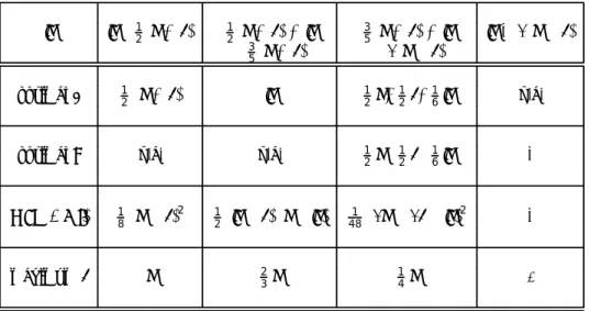
¹₂

. The tax is linear. The market maker can take the following strategies: Table 3.1 summarizes the results.

1. The market maker can exclude the informed trader by setting the selling price above the latter’s maximum valuation; a

≥

v. By having no informed trader, the dealer imposes ¯ no quantity limit, z. In this case, the market maker is a monopolist facing a downward sloping curve and his expected proÞt is

E[π] = E

·

I[d(a)

≥

0] d(a)

¸

(a

−

c) = E

·

I[η

≥

a] (η

−

a)

¸

(a

−

c) = 1

2 (¯

η−

a) (a

−

c).

The proÞt-maximizing price, (c + ¯

η)/2

is the listed price provided this price is above v ¯ and the maximum value for the proÞt is

¹₈

(¯

η−

c)

²

. To summarize when a

≥

v: the optimal ¯ price that excludes the informed trader is max[¯ v, (c + ¯

η)/2]; there is no quantity limit; the

maximum expected proÞt is

¹₈

(¯

η−

c)

²

; and the maximum amount of tax is

η.

¯

2. Alternatively, the market maker can set his selling price below ¯ v in the hope of attracting more demand; 0 < a < ¯ v.

⁴

Naturally, he then runs the risk of being picked by the informed trader. Given a selling price a,

η

¯

−a

is the highest possible liquidity demand.

⁵

If the dealer set the depth strictly above this level, he would incur extra losses when transacting with

4If0< a <¯vthenI[v≤a] =I[v=−¯v],I[v > a] =I[v= ¯v].

5We impose a≤¯ηsince settingaabove¯η would make the liquidity demand always negative, and hence the liquidity trader would not trade in this case.

5

the informed without generating extra liquidity trade. Hence, z

· η

¯

−

a. When the liquidity demand is positive, it is equal to the quantity limit. Consequently, the expected proÞt is:

E[π] = E[I[v

·

a](a

−

c

−

v)] E[I[d(a)

≥

0] z] + E[I[v > a](a

−

c

−

v)] z

=

µ

E[I[v

·

a](a

−

c

−

v)] p(d(a)

≥

0) + E[I[v > a](a

−

c

−

v)]

¶

z

=

µ

1

4

(a + ¯ v

−

c) +

¹₂

(a

−

v ¯

−

c)

¶

z

=

³₄

z(a

−

c

−¹₃

¯ v)

(3.1)

If a < c + ¯ v/3, the optimal z is 0; if a > c + ¯ v/3, the optimal z is the maximum quantity limit ¯

η−

a; if a = c + ¯ v/3, z can be set arbitrarily, for example, to zero.

With z = ¯

η−

a, the expected proÞt function becomes:

E[π] = 3

4 (¯

η−

a) (a

−

c

−

1

3 v). ¯ (3.2)

The dealer maximizes the function deÞned in Equation (3.2) under the constraint that 0 < a < v. If ¯ v > ¯ 3 (¯

η−

c), this function is negative for a < ¯

η

and the dealer exits the market. If ¯ v

·

3 (¯

η −

c), the price that maximizes E[π] without the constraint a < ¯ v,

1

2

(c + ¯

η) + ¹₆

v, is smaller than ¯ v ¯ if v > ¯

³₅

(¯

η

+ c). Hence, if

³₅

(c + ¯

η)

< ¯ v

·

3 (¯

η−

c), the optimal price is

¹₂

(¯

η

+ c)+

¹₆

¯ v and the maximum proÞt is

₄₈¹

(3¯

η−

3c

−

v) ¯

²

; if ¯ v

·³₅

(c+ ¯

η

), the constraint a < ¯ v is binding; in the limit, the dealer wants to set a = ¯ v.

The

Þnal step is to compare the maximum expected proÞt when

a > ¯ v and when a

·

¯ v.

When

³₅

(¯

η

+ c) < v < ¯ 3 (¯

η−

c), maximizing expected proÞt setting a

≥

v ¯ would yield a lower

6

Table 3.1: Equilibrium price and quantity limit with risk-neutral informed trader and discrete distributions.

¯

v ¯ v

·¹₂

(¯

η

+ c)

¹₂

(¯

η

+ c) < v ¯

³₅

(¯

η

+ c) < v ¯ v > ¯ 3(¯

η−

c)

·³₅

(¯

η

+ c)

·

3(¯

η−

c)

optimal

a

¹₂

(¯

η

+ c) v ¯

¹₂η+

¯

¹₂

c+

¹₆

v ¯

n.a.

optimal

z

n.a. n.a. ¹₂η−

¯

¹₂

c−

¹₆

v ¯ 0

max (E [π])

¹₈

(¯

η−

c)

^{2 1}₂

(¯ v

−

c) (¯

η−

¯ v)

₄₈¹

(3¯

η−

3c

−

¯ v)

²

0

maximum

c

η

¯

²₃

¯

η ¹₄

¯

η 0

When

a

≥

¯ v

, imposing a quantity limit is not necessary; the optimal

z

is undeÞned and “n.a.” is entered in the corresponding cell. When

v > ¯ 3 (¯

η−

c)

, the expected proÞt is never positive and the dealer exits the market by setting

z

to

0

; the optimal

a

is undeÞned and “n.a.” is entered in the corresponding cell.

maximum than letting a < ¯ v. The optimal price and depth in this case are a

^∗

=

¹₂

(¯

η

+ c) +

¹₆

¯ v and z

^∗

= ¯

η−

a

^∗

. When

¹₂

(¯

η

+ c) < v ¯

· ³₅

(¯

η

+ c), the optimal price is

ν

and no quantity limit need be imposed. When ¯ v

≥

3(¯

η−

c), the depth is set to zero and no price need be quoted.

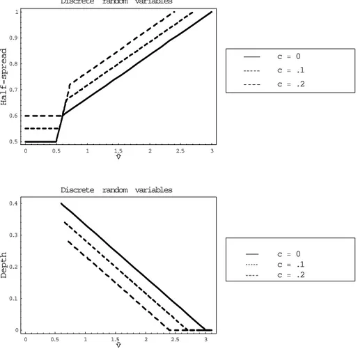
For expositional purpose, Figure 3.1 maps the results in Table 3.1. Figure 3.1 plots the half spread, a, and the depth, z, against the informed trader’s valuation, v. ¯ The main message from Figure 3.1 is that the introducing of a transaction cost has non-linear effects on the spread and the depth. When the random variables follow discrete distributions, imposing a

Þnite depth is

not necessary if the asymmetry in information is low enough. For example, in the region where

¯ v

∈ ¡

0,

³₅¢

, a small increase in the transaction cost pushes up the spread but does not affect

7

the depth

⁶

, while a larger change may result in the imposition of a

Þnite quantity limit but

may not translate into a spread increase of equal magnitude. In contrast, when the information asymmetry is more severe, v ¯

∈¡₃

5

, 3

¢

, and the quantity limits are imposed, an increase in the transaction cost has a proportional effect on the spread.

4. Equilibrium with continuous distributions

In the following section, we take the asset value, x, to be lognormally distributed. With the lognormal distribution, the demand is d(a) =

−

log(a) +

η

and y = log(x). We also assume that the distribution of (x,

η, G)

is common knowledge with

η

and G are normally distributed.

4.1. Marginal condition

Although no equilibrium closed-form solution exists, the marginal conditions for the price and the quantity limit shed light on the trade-offs governing the dealer’s proÞt maximization.

The

Þrst derivative of the specialist’s expected proÞt with respect to the quantity limit is

given in Equation (4.1); the one with respect to the ask price is given in Equation (4.2), where d

⁰

(a) denotes the slope of the liquidity demand at price a.

⁷

∂

∂z

E[π] = p(d(a) > z) E

·

I[v

·

a] (a

−

c

−

v)

¸

+ E

·

I[v > a] (a

−

c

−

v)

¸

, (4.1)

∂

∂a

E[π] = p(v > a) z + p(v

·

a) E

·

I[d(a)

≥

0] min(d(a), z)

¸

+ d

⁰

(a) p(0

·

d(a)

·

z) E

·

I[v

·

a] (a

−

c

−

v)

¸

.

(4.2)

6In fact, the depth in this region is “undeÞned”.

7The derivation of equations (4.1) and (4.2) can be provided upon request.

8

0 0.5 1 1.5 2 2.5 3

v¯

0 0.1 0.2 0.3 0.4

htpeD

Discrete random variables

c = .2 c = .1 c = 0

0 0.5 1 1.5 2 2.5 3

v¯

0.5 0.6 0.7 0.8 0.9 1

flaH−daerps

Discrete random variables

c = .2 c = .1 c = 0

Figure 3.1:

Half-spread and depth when the informed trader’s valuation and the liquidty shock each take two values with probability 1/2. The positive value of the liquidity shock is 1, that of the in- formed trader’s valuation is

v

and is displayed on the horizontal axis. ThisÞgure represents the market conditions facing the dealer.

9

Equation (4.1) has an intuitive interpretation. Increasing the quantity limit by an inÞnitesimal amount brings the market maker a proÞt equal to E

·

I[v

·

a] (a

−

c

−

v)

¸

if the limit is hit by a liquidity trader, or a loss equal to E

·

I[v > a] (a

−

c

−

v)

¸

if it is hit by an informed trader.

Equation (4.2) is similar to the standard monopolistic case in which increasing the price by $1 makes the monopolist earn another $1 on the total volume but reduces the overall demand.

The

Þrst two terms on the right-hand side of Equation (4.2) represent the expected sales when

the informed trader wants to trade, p(v > a) z, and when he does not, p(v

·

a) E

·

I[d(a)

≥

0] min(d(a), z)

¸

. The last term represents the impact on proÞts resulting from the reduction in overall demand. A price increase depresses demand if the quantity limit is not binding, that is, if the liquidity trader’s demand is positive but lower than z and the informed trader’s evaluation is below a. In this event, the effect on overall demand is proportional to the slope of the liquidity trader’s demand.

4.2. Expected dealer’s profit

We assume that the informed trader is endowed with a negative exponential utility function with risk aversion

γ. Equivalently, the informed trader maximizes

E[π

ⁱ|G]−γ

var(π

ⁱ|G)/2, whereπⁱ

is the informed trader’s proÞt and var(π

ⁱ|G)

is the conditional variance of his proÞt given G.

We assume that his initial wealth is conditionally independent of the value of the asset and the liquidity shock. The informed trader chooses the quantity q to maximize

q (E[x|G]

−

a

−

c)

−

1

2 q

²γ

var(x|G), (4.3)

10

where var(x|G) is the conditional variance of x given G. As the informed trader’s orders are

Þlled before those of the liquidity trader, the informed trader’s demand function is

q(a) = max

·

0,

µ

γ

var(x|G)

¶−1

(v

−

a

−

c)

¸

, (4.4)

with var(x| G) =

σ²_x

(1

−ρ²

). When x is lognormally distributed, this is not linear in v be- cause the conditional variance of x given G depends on the realization of G: var(x|G) =

£

exp

¡

(1

−ρ²

)σ

²_y¢

−

1

¤

v

²

, where

σy

is the standard deviation of y = log(x) and

ρ

= corr(G, y).

⁸

Thus, the informed trader’s demand is deÞned by

q(a, c, v) = 1

θ

max[0, 1

v

−

a + c v

²

],

where

θ

=

γ £

exp

¡

(1

−ρ²

)σ

²_y¢

−

1

¤

.

4.3. Numerical Results

When x is lognormally distributed, we search for the optimal price (or spread) and for the optimal depth numerically. The dealer’s proÞt maximization simpliÞes to a one-dimensional problem when the informed trader is risk neutral because the optimal depth in this case can be written as a function of the spread.

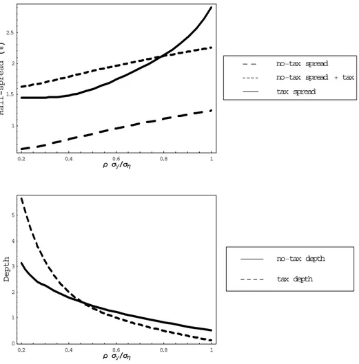
Figure 4.1 graphs the half-spread and depth, both divided by

ση

, against against

ρ σy

/σ

η

when x is lognormally distributed and

ση

= 0.1.

⁹

Figure 4.1 uses a logarithmic scale for the

8To compute the conditional variance in the lognormal case, usevar(x|G) =E[x²|G]−E[x|G]²together with the fact thatlog(x),log(x²), andGare jointly normally distributed.

9Note that note thatv¯=ρ σyand¯η=ση. Consequently, an increase inρ σy/σηrepresents an increase in the degree of asymmetric information: the valuation of informed trader increase, which translates into an unfavorable market condition for the dealer.

11

vertical axis. As in the discrete case, introducing a transaction cost has non-linear effects on the spread and the depth and the effect depends on whether market conditions are favorable or unfavorable to the dealer.

The spread increases and the depth decreases with

ρ σ_y

/σ

_η

. When market conditions are very favorable - that is, the informed trader is poorly informed - the depth grows without bound while the spread remains

Þnite because of the dealer’s market power. When market conditions

become very unfavorable, the dealer exits the market by setting the depth to 0 while maintaining a

Þnite spread. When

x is lognormally distributed, half-spread and depth are approximately proportional to

σ_η

. For example, for

ρ σ_y

/σ

_η

= 0.5, the half-spread equals about 0.8 percent when

σ_η

= 0.01 and 9 percent when

σ_η

= 0.1.

¹⁰

When market conditions are favorable to the dealer (e.g.

ρ σ_y

/σ

_η ∈

(0.2, 0.4)), introducing a transaction cost increases the spread by less than the amount of the transaction cost and creates a larger depth. On the other hand, when market conditions are unfavorable to the dealer (e.g.

ρ σy

/σ

η ∈

(0.8, 1.0)), introducing a transaction cost pushes the price up by more than the transaction cost and narrows the depth.

Furthermore, for both the discrete and continuous cases, the strength of the liquidity demand plays a central role in determining the equilibrium spread and depth. When studying the market marking process, one can focus on the liquidity conditions the dealer faces rather than on information asymmetry. This is particularly suited to the U.S. government bond market.

For example, spreads are typically narrower and depth larger for securities that are the most recent issues in their maturity class (the on-the-run Treasuries) than for similar securities issued

1 0Making the informed trader risk averse and choosing different volatilities for the asset and the liquidity shock do not qualitatively affect the results.

12

0.2 0.4 0.6 0.8 1

ρ σyêση 0

1 2 3 4 5

htpeD tax depth

no₋tax depth

0.2 0.4 0.6 0.8 1

ρ σyê^ση 1

1.5 2 2.5

flaH−daerpsH%L

tax spread

no₋tax spread ₊tax no₋tax spread

Figure 4.1:

Half-spread (in percentage) and depth with a proportional transaction cost of 1 percent (solid line) and without transaction cost (short-dashed line). The asset value,

x

, is lognormally distrib- uted and

y = log(x)

. In the top panel, the long-dashed line is the sum of the price without transaction cost and the transaction cost. Half-spread and depth are divided by ση.

13

just before (the off-the-run Treasuries). Bid-ask spreads on coupon Treasury securities have traditionally been about twice as high for off-the-run issues than for comparable on-the-run issues, while quoted depth is lower. Moreover, during the recent bouts of market volatility, bid- ask spreads have widened and depth has contracted proportionally more for off-the-run than for on-the-run coupon securities. The asymmetric information argument cannot easily account for this fact since the quality of private information should be equal across the two market segments. However, agents trading bonds prefer to trade in the on-the-run securities, therefore creating a stronger liquidity demand in that market. The more fundamental question as to why agents prefer to trade in the on-the-run segment is not addressed here, although self-fulÞlling expectation arguments could be made.

The paper seems to point to two regimes as far as transaction cost is concerned. When market conditions are favorable, the dealer pays part of the transaction cost himself (by increasing the spread less than the cost) and quotes a larger depth to attract order

ßow in order to make

up for the loss in demand due to the transaction cost. The increase in the depth offsets, albeit partially, the effect on trading volume of the wider spread. When market conditions are unfavorable, increasing the transaction cost leads to a drastic reduction in the liquidity provided by the market maker, enticing him to exit the market.

Although, the implications of the model have been introduced by presenting the effect on the spread and the depth of an increase in the transaction cost, symmetric conclusions hold for a reduction in this cost. As a consequence, a decision to lower taxes on transactions in the hope of improving market liquidity might actually lead to smaller depths and a less-than-proportional reduction in the spreads. This is because, when market conditions are rather favorable to the dealer, a tax–insofar as it is at least partially reßected in the bid and ask prices–reduces the

14

probability of the informed trader’s buying at the ask or selling at the bid. This additional protection entices the market maker to quote a larger depth than he would without tax.

5. Conclusion

The model shows that introducing a transaction tax could affect market liquidity differently depending on the market conditions facing the dealer. If the asset value, the informed trader’s signal, and the liquidity shock each take two values, there is an interval for the precision of the private signal for which increasing the transaction tax has no or little effect on the spread (no quantity limit is necessary then). If the asset value is lognormally distributed, the market maker widens the spread by less than the transaction tax and actually increases the depth when the degree of information asymmetry is subdued or liquidity demand is strong. In contrast, when market conditions are unfavorable to the dealer, he increases the spread by more than the transaction tax and reduces the depth. For all distributions, introducing a transaction tax may induce the dealer to exit the market before he would have done so in the absence of a transaction tax. This suggests that a transaction tax could aggravate liquidity loss in periods of market stress.

15

References

[1] Barclay, Michael-J, Eugene Kandel, and Leslie-M Marx, (1998), ”The Effects of Transaction Costs on Stock Prices and Trading Volume”,

Journal of Financial Intermediation, Vol. 7(2),

pg. 130-50.

[2] Brennan, Michael-J, Tarun Chordia, Avanidhar Subrahmanyam, (1998), ”Alternative Fac- tor SpeciÞcations, Security Characteristics, and the Cross-Section of Expected Stock Re- turns”,

Journal of Financial Economics, Vol. 49(3), pg. 345-73.

[3] Constantinides, George-M, (1986), ”Capital Market Equilibrium with Transaction Costs”,

Journal of Political Economy, Vol. 94(4), pg. 842-62.

[4] Dow, James and Rohit Rahi, (2000), ”Should Speculators Be Taxed”, Journal of Business, Vol. 73(1), pg. 89 - 107.

[5] Dupont, D. , (2000), “Market making, prices, and quantity limits,”

Review of Financial Studies

, Vol. 13(4), pg. 1129-1151.

[6] Hakkio, C.S., (1994), ”Should we throw sand in the gears of

Þnancial markets”, Federal

Reserve Bank of Kansas City,

Economic Review, Vol. 79 (2), pg. 17 - 30.

[7] Glosten, L., and P. Milgrom, (1985), “Bid, Ask and Transaction Prices in a Specialist Market with Heterogeneously Informed Traders,”

Journal of Financial Economics, Vol. 14,

pg. 71-100.

[8] Kadlec, Gregory-B and John-J McConnell, (1994), ”The Effect of Market Segmentation and Illiquidity on Asset Prices: Evidence from Exchange Listings”, Vol. 49(2), pg. 611-36.

16

[9] Vayanos, Dimitri, (1998), ”Transaction Costs and Asset Prices: A Dynamic Equilibrium Model”,

Review of Financial Studies, Vol. 11(1), pg. 1-58.

[10] Vayanos,-Dimitri and Jean-LucVila, (1999), ”Equilibrium Interest Rate and Liquidity Pre- mium with Transaction Costs”,

Economic Theory, Vol. 13(3), pg. 509-39

17

Authors: Dominique Y. Dupont, Gabriel S. Lee

Title: Effects of Securities Transaction Taxes on Depth and Bid-Ask Spread Reihe Ökonomie / Economics Series 132

Editor: Robert M. Kunst (Econometrics)

Associate Editors: Walter Fisher (Macroeconomics), Klaus Ritzberger (Microeconomics)

ISSN: 1605-7996

© 2003 by the Department of Economics and Finance, Institute for Advanced Studies (IHS),

Stumpergasse 56, A-1060 Vienna • +43 1 59991-0 • Fax +43 1 59991-555 • http://www.ihs.ac.at

ISSN: 1605-7996