Policy Research Working Paper 6055
Gender, Geography and Generations
Intergenerational Educational Mobility in Post-reform India
M. Shahe Emran Forhad Shilpi
The World Bank
Development Research Group
Agriculture and Rural Development Team May 2012
WPS6055
Public Disclosure Authorized Public Disclosure Authorized Public Disclosure Authorized Public Disclosure Authorized
Produced by the Research Support Team
Abstract
The Policy Research Working Paper Series disseminates the findings of work in progress to encourage the exchange of ideas about development issues. An objective of the series is to get the findings out quickly, even if the presentations are less than fully polished. The papers carry the names of the authors and should be cited accordingly. The findings, interpretations, and conclusions expressed in this paper are entirely those of the authors. They do not necessarily represent the views of the International Bank for Reconstruction and Development/World Bank and its affiliated organizations, or those of the Executive Directors of the World Bank or the governments they represent.
Policy Research Working Paper 6055
India experienced sustained economic growth for more than two decades following the economic liberalization in 1991. While economic growth reduced poverty significantly, it was associated with an increase in inequality. Does this increase in inequality reflect deep- seated inequality of opportunity or efficient incentive structure in a market oriented economy? This paper provides evidence on economic mobility in post-reform India by focusing on the educational attainment of children. It uses two related measures of immobility:
sibling and intergenerational correlations.
The paper analyzes the trends in and patterns of educational mobility from 1992/93 to 2006, with a special emphasis on the roles played by gender and
This paper is a product of the Agriculture and Rural Development Team, Development Research Group. It is part of a larger effort by the World Bank to provide open access to its research and make a contribution to development policy discussions around the world. Policy Research Working Papers are also posted on the Web at http://econ.worldbank.org.
The author may be contacted at fshilpi@worldbank.org.
geography. The evidence shows that family background
plays a strong role; the estimated sibling correlation in
India in 2006 is higher than the available estimates for
Latin American countries. There is a persistent gender
gap in rural and less-developed areas. The only group
that experienced substantial improvements is women
in urban and developed areas, with the lower caste
women benefiting the most. Almost 70 percent of the
variance in children’s education can be accounted for by
parental education and geographic location. The authors
provide possible explanations for the apparently puzzling
improvements for urban women in a country with strong
son preference.
Gender, Geography and Generations:
Intergenerational Educational Mobility in Post-reform India
M. Shahe Emran 1
IPD, Columbia University
Forhad Shilpi
DECRG, World Bank
JEL Codes: O12, J62
Key Words: Intergenerational Mobility, Education, Equality of Opportunity, Sibling Correlation, Intergenerational Correlation, Economic Liberalization, Rural-Urban Inequality, Gender Gap, India
1
We would like to thank Will Martin, Giovanna Prennushi and Debdulal Mallick for comments on an earlier draft.
Emails for correspondence: shahe.emran@gmail.com (M. Shahe Emran) and fshilpi@worldbank.org (Forhad
Shilpi).
2 (1) Introduction
The increasing inequality in income distribution at a time of considerable economic growth during the last couple of decades has rekindled interests in intergenerational mobility in both developed and developing countries.
2Following wide ranging economic liberalization in the early 1990s, India experienced sustained high economic growth; per capita GDP grew at a 4 percent rate over the two decades after liberalization. The evidence indicates that while growth led to a significant poverty reduction, it was also associated with a rise in inequality (World Bank (2011)).
3There is increasing concern that the benefits of economic growth were not shared broadly, and remained especially concentrated in urban areas, thus widening the rural-urban gap (Bardhan (2007, 2010), Dreze and Sen (2011), Basu (2008), Prasad (2012)).
4The estimates of top incomes by Banerjee and Piketty (2005) show that the share of top 0.01, 0.1, and 1 percent in total income has increased substantially from a trough in the mid1980s, and this increase coincided with the move away from ‗Socialist‘ to more market oriented economic policies. According to their estimates, in 1999-2000, per capita income gap between the 99
thand 99.5
thpercentiles was four times as large as the gap between the median and the 95
thpercentile. Another recent study finds that between 1996 and 2008, the wealth holding of the Indian billionaires increased from 0.8 percent of GDP to 23 percent, before declining to 14 percent in 2010 (Walton (2010)).
52
Among the developing countries, China and India are two prominent examples where impressive economic growth
has been accompanied by an increase in inequality. For a discussion on rising inequality in Asia, see Jushong and Kanbur (2012). The recent decline in intergenerational mobility in USA and UK has also attracted a lot of attention;
see, for example, Deparle in New York Times (January 4, 2012) and Mazumder (2012) on USA, and Dearden et al.
(1997) and Blanden et al. (2005) on UK.
3
For evidence on rising inequality in India after 1991, see Ravallion (2000), Deaton and Dreze (2002), Sen and
Himanshu (2004). A recent survey of the available evidence shows that consumption inequality has increased slightly, but the income inequality in India is much higher than what is usually thought of (close to Brazil) (World Bank (2011)). It is now widely appreciated that the available estimates of consumption and income inequality may be significantly biased downward, because the household surveys fail to cover the top income households.
4
Dreze and Sen (2011) argue that Indian economic reform has been an ―unprecedented success‖ in terms of economic growth, but an ―extraordinary failure‖ in terms of improvements in the living standards of general people and social indicators.
5
The volatility in the wealth of billionaires reflects the volatility in the stock market. The common perception about
a significant increase in inequality is reinforced by spectacular conspicuous consumption by the super-rich: Mukesh
Ambani, the chairman of Reliance Industries in India owns and lives in the first billion dollar house in the world
(Woolsey, M, Forbes.com, April 30, 2008), and in the mega wedding of two sons of Subrata Roy, the ‗chief
3
However, the relevant question is whether the observed increase in cross-sectional inequality is a natural outcome of efficient incentive structure in a liberalized and market oriented economy that rewards hard work and entrepreneurial risk taking, or it is primarily due to inequality of opportunity due to differential access, for example, to education and markets. The rise in cross-sectional inequality becomes a serious concern when it is primarily a result of inequality of opportunity, i.e., the inability of children born in poorer families and disadvantaged social groups to move beyond their parents‘ position in economic ladder by their own effort and choices.
6An immobile society may require policies, public investments and reforms to ensure both efficiency and equality of opportunity.
7Understanding the trends in and the levels and patterns of intergenerational mobility during the post liberalization period has thus become important for academics and policy makers (Bardhan (2010), Banerjee and Piketty (2005)).
8This paper provides evidence on intergenerational economic mobility in India during the post liberalization period by focusing on the educational attainment of children. Education is used as an indicator of economic status in the absence of suitable data on permanent income.
9There is a broad consensus in the literature that education is among the most important avenues for poor to escape from poverty traps and climb up the economic ladder (for recent surveys, see Orazem and King (2008), Strauss and Thomas (1995)). The role of education may be especially important in post- reform India where growth has been concentrated in skill intensive sectors: the software industry and call centers being iconic examples (Kochhar et al. (2006), Bardhan (2010), Kotwal et al. (2011)).
10The goal of this paper is to analyze the trends in and levels and patterns of educational mobility over guardian‘ of Sahara Group, $ 250,000 was spent on candles alone (Srivastava, S, BBC online, February 11, 2004)!
The popular perception that rural areas in India have been largely left out of the recent economic growth is, at least partly, shaped by the reports of farmers‘ suicides, among other things.
6
Higher inequality of opportunity is likely to lead to a higher cross-sectional inequality (Atkinson (1981)). Many
observers believe that inequality in India reflects inequality in opportunity. For example, Basu (2008) comments that
―A certain amount of inequality may be essential to mitigate poverty….But the extent of Inequality in India seems to be well above that‖.
7
In an immobile society, many high ability children from poor families may not be able to go to school and thus fail
to realize their productive potential. High inequality can also lead to political instability.
8
For a broader discussion on the importance of equity in economic opportunity for development, see Equity and
Development (World Development Report (2006)).
9
Reliable data on children‘s and parents‘ income over the life cycle are not available in a developing country such as India. As emphasized in the recent literature, one needs good quality income data over a number of years at appropriate phase of the lifecycle to tackle the attenuation bias in the estimated intergenerational correlation in income (Solon (1999), Mazumder (2003)). The analysis of intergenerational persistence in income in India is also complicated by the fact that a majority of population especially during parent‘s generation were engaged in family farming as self-employed workers making it difficult to attribute income to individual members.
10
This is in contrast to the Chinese experience where growth has been dominated by agriculture and labor intensive
manufacturing. Bardhan (2010) and Datt and Ravallion (2010) emphasize low and unequal human capital as an
important constraint on poverty reduction in India.
4
a period of almost a decade and a half after the liberalization in 1991 (1993-2006), with a special focus on possible gender and spatial differences (rural vs. urban and developed vs. less-developed states). We use two related measures of educational immobility: (1) sibling correlation in educational attainment and (2) persistence in educational attainment across parents and children. The standard approach to the study of intergenerational educational mobility is to estimate the parent- offspring association in educational attainment.
11It has, however, been well appreciated in the literature that the influence of family background on children extends much beyond what is implied by parent‘s education (Corcoran et al. (1990), Mazumder (2008, 2011, 2012), Bjorklund, Lindahl and Lindquist (2010), Bjorklund and Salvanes (2010)). Sibling correlation is a much broader concept that provides a summary measure of all common family and community background factors that affect child outcomes but are not chosen by children themselves.
12A significantly higher sibling correlation implies greater influence of family and community backgrounds on economic outcomes, which in turn indicates that the role one‘s own effort and choices can play is limited. To the best of our knowledge, there is no study in the literature that exploits estimates of both sibling correlations and intergenerational correlation to trace out the levels, trends in and patterns of intergenerational mobility in a developing country.
There is now a large and mature literature on intergenerational economic mobility in developed countries, most of which focuses on intergenerational correlation between parents‘ and children‘s incomes (for reviews, see Solon (1999, 2002), Black et al. (2010)).
13However, economic analysis of intergenerational mobility in the context of developing and transitional countries remains a largely unexplored area of research (among the available contributions, see Jalan and Murgai (2008), Hnatkovska et al. (2011), Dahan and Gaviria (2001), Emran and Shilpi (2011), and Emran and Sun (2011)). Also, the existing economic literature on sibling correlation in education focuses primarily on a set of developed countries that include USA, UK, Norway and Sweden. The only exception known to us is Dahan and Gaviria (2001) who provide estimates of sibling correlations for 16 Latin American countries. They find that El Salvador, Mexico, Colombia and Ecuador are the least mobile countries, with sibling correlation explaining almost 60 percent of the variation in
11
For a survey of this literature, see Black and Devereux (2010), Bjorklund and Salvanes (2010) for developed countries, and Hertz et al. (2009) for developing countries.
12
It is, however, important to recognize that parent-children correlation is not a proper subset of the sibling
correlation in representing the effects of family background on economic outcomes. The intergenerational link between the parents and a child captures genetic similarities that may not be shared by the siblings, except for the identical twins.
13
See, among others, Arrow et al. (2000), Dearden et al. (1997), Mulligan (1999), Solon (1999, 2002), Birdsall and
Graham (1999), Fields et al. (2005), Bowles et al. (2005), Blanden et al. (2005), World Development Report (2006),
Mazumder (2003), Hertz (2005), Bjorklund et al. (2006), and Lee and Solon (2009).
5
educational outcomes. The available evidence on developed countries shows that factors common to siblings explain from 40 to 65 percent of variation in educational outcomes (Bjorklund and Salvanes (2010)). In contrast, intergenerational correlation between parents and children– the traditional measure of intergenerational persistence -- explains from 9 to 21 percent of variations in children‘s educational outcome. An interesting finding from these studies is that gender or geographic location (as measured by neighborhood effect) does not exert any significant influence on the intergenerational persistence in children‘s educational outcomes. Are gender and geography also largely irrelevant for educational mobility faced by children in developing countries? One can argue that the role of gender and geography might be much more prominent in a developing country such as India, because gender bias against women is more common and stronger, geographic mobility is lower, and many areas (especially rural) are not integrated with the urban growth centers because of underdeveloped transport infrastructure.
14On the other hand, the high tide of rapid economic growth in Indian economy for more than two decades may have lifted all the boats, improving economic mobility across the income distribution, irrespective of gender and geographic location.
The data used in this paper come from the1992/93 and 2006 rounds of the National Family Health Survey (NFHS) in India. The first period of our sample nearly overlaps with the period of economic liberalization (1991-1992), and the second period is about 15 years after liberalization. For both survey rounds, our analysis focuses on the same age cohort (16 to 27 year olds) who constitute the bulk of new entrants into the labor force.
15To examine the spatial aspects in detail, the empirical analysis is done separately for families residing in different areas such as rural vs. urban areas and relatively developed vs. less developed states. To discern any possible gender bias, we implement the empirical analysis separately for male and female samples. We use the mixed effects model to estimate the sibling correlation. An advantage of this approach is that both the family and community level covariates can be included in the analysis to examine their relative influence on sibling correlation (Mazumder (2008), Bjorklund et al. (2011)). We examine the influence of two sets of covariates on sibling and intergenerational correlations: the first set relates to caste and religion of the
14
There is evidence that geographic location may be important for economic opportunities faced by households in
developing countries. For example, Jalan and Ravallion (1999) show that there are geographic poverty traps in China. Emran and Hou (forthcoming) find that better access to markets increases household consumption in rural China in a significant way. They also find that the effects of domestic market centers are much larger than that of international market access.
15
Our conclusions, however, do not depend on this particular age cohorts. In the robustness checks section, we
provide evidence using an alternative age cohort sample.
6
household which are identified as important determinants of educational attainment in India, and the second relates to the geographic location as measured by neighborhood fixed effect.
16Our estimates of sibling and intergenerational correlations suggest no significant change in the intergenerational persistence in educational attainment for a large proportion of the population in India from 1992/93 to 2006. Sibling (and intergenerational) correlations in our full sample have declined only marginally from 0.64 (0.57) in 1992/93 to 0.62 (0.54) in 2006 respectively.
17However, this aggregate picture hides important gender and spatial differences. While the evidence indicates that the sibling correlation among men (brothers) has remained effectively unchanged (it increased slightly from 0.614 in 1993 to 0.624 in 2006), it experienced a moderate decline for women, (sisters) from 0.780 to 0.696. Geographic location is important, both in 1992/93 and 2006;
the neighborhood effect accounts for about 40 percent of the sibling correlation among women and a third among men. In terms of geographic pattern, we find that sibling correlation remained essentially unchanged in rural areas and declined marginally in urban areas. The sibling correlation also declined slightly in the developed states, but increased in the less-developed states. Perhaps the most interesting trends and patterns emerge when we partition the data using both gender and geography. The sibling correlations among men (brothers) in rural areas and less-developed states have increased a bit, but the correlation has in fact declined marginally in urban areas and remained virtually constant in developed states. In contrast, the sibling correlations among women (sisters) registered a decline irrespective of geographic partitioning of the data. However, geography matters for women also, only the women in urban areas and developed states experienced substantial decline in sibling correlations. As a result, the gender gap in sibling correlation has disappeared in urban areas though it remains virtually unchanged in rural areas. We also find that among the urban women, it is the lower caste women who experienced the largest decline in the sibling correlation.
The evidence on improvements in educational mobility of women is similar to the available evidence on China and Malaysia (see Emran and Sun (2011) on China and Lillard and Willis (1994) on
16
The recent evidence using NSS data shows that the influence of caste and religious identity on the strength of
intergenerational link between parents and children has become much weaker (Hnatkovska et al. (2011)). Our results also show a similar pattern. It is however, important to note that the direct effect of lower caste and Muslim dummy remains significantly negative on children‘s educational attainment.
17
Note that a formal test of equality of the estimates in 1993 and 2006 rejects the null because of very small
standard errors due to the large sample sizes (number of observations is 34000 in 1993 and 38000 in 2006).
However, statistical precision is largely irrelevant here, because the difference in the numerical magnitude of the
estimates between 1992/93 and 2006 is very small in most of the cases, suggesting the lack of any substantial
change in intergenerational mobility over a period of almost a decade and a half of impressive economic growth.
7
Malaysia).
18The broad trends in and patterns of educational persistence discussed above are also observed in the estimates of intergenerational correlations in education between parents and children.
In contrast to the evidence from developed countries, majority of the variations in sibling correlations in India can be explained by two factors: parental education and geographic location as measured by neighborhood effect.
The estimates indicate that a decade and a half after the economic liberalization in 1991, the absolute magnitudes of sibling and intergenerational correlations in India in 2006 are still very large, larger than the available estimates for the Latin American countries (for sibling correlations) and Asian countries (for intergenerational correlations). The influence of family and community backgrounds is especially dominant for rural women: about 70 percent of variations in sisters‘
schooling levels can be explained by common family and community factors shared, but not chosen, by them. After more than two decades of impressive economic growth, a large proportion of Indian population experienced no significant change in their educational opportunity; place of residence and gender still play a large role in a child‘s educational attainment and thus his/her economic fortunes.
The absence of a positive effect of economic growth on educational mobility, especially for men, is, however, not peculiar to the Indian experience following liberalization. Recent evidence shows that educational mobility of men in rural China has in fact worsened during the high growth post reform period (1988-2002) (Emran and Sun (2011)).
The rest of the paper is organized as follows. The conceptual framework underpinning empirical work is described in section 2. Data and empirical strategy are elaborated in section 3.
Section 4 organized in different subsections presents the main empirical results, and section 5 reports as set of robustness checks. Some preliminary conjectures for explaining the observed trends in and patterns of educational mobility in post-reform India are offered in section 6. The paper concludes with a summary of the findings.
(2) Conceptual Framework Sibling Correlation (SC)
For the estimation and interpretation of sibling correlations, we adopt a conceptual framework that has been utilized widely in the empirical literature on sibling correlations (see, Solon et al (1991), Bjorklund et al (2002), Bjorklund and Lindquist (2010), Bjorklund and Salvanes (2010),
18
The positive evidence on women may seem puzzling given the fact that son preference is prevalent in all three
countries. We provide a set of explanations for the observed trend later in the paper.
8
Mazumder (2008) and (2011)). )). Let
be the years of schooling of sibling j in family i. It can be expressed as:
(1)
where is a family component which is common to all siblings in family i and
is the individual specific component for sibling j which captures j‘s deviation from the family component. Assuming these two components are independent, the variance of
can be expressed as the sum of variances of the family and individual components as:
(2) The sibling correlation in education then can be expressed as:
(3)
The sibling correlation depicts the share of variance of years of education that can be attributed to common family background effects. Thus sibling correlation can be thought of as a summary statistic measuring the importance of common family and community effects which includes anything and everything shared by the siblings. It is useful to distinguish among different types of family and community factors that are commonly experienced by siblings. The family level variables include observable factors such as parental education and occupation as well as unobserved factors such as common genetic traits, parental aspirations, child rearing ability and style, cultural inheritances and interaction among siblings. The community effects include factors such as school availability and quality as well as peer effects within the neighborhood. Though sibling correlation captures most of the family background influences, it does not capture all of them. For instance, genetic traits not shared by siblings, differential treatment of siblings and time dependent changes in family and neighborhood factors will show up in the individual component of outcome variance, though they might be part of family background. As a result, the estimate of sibling correlations can be taken as a lower bound estimate of the total influence of the common family background on children‘s education outcome (for a discussion on this point, see Bjorklund and Salvanes (2010)).
Intergenerational Correlation (IGC)
It is instructive to look at the difference between sibling correlations and intergenerational
correlations as measures of intergenerational persistence in economic outcomes. The standard
9
regression model to estimate intergenerational correlation between parents and children can be written as:
(4)
where is the parental year of schooling in family i, and is the intergenerational regression coefficient. Because individual component in equation (1) is orthogonal to the family component, one can express the family component as:
(5)
where denotes family factors that are orthogonal to parental education. It follows from equation (5) that:
where
is the intergenerational correlation in education. The above equation shows clearly that sibling correlation is a broader measure of the impact of family background than the squared
intergenerational correlation. Also, the intergenerational correlation parameter (
) is different from intergenerational regression coefficient ( ).
Estimating Equations
To estimate the sibling correlations, we extend the regression model in equation (1) and specify the following mixed effects model:
(6)
where
is a vector of control variables. To estimate the intergenerational correlation in education, we augment equation (4) to estimate the following regression specification where the education variables of both generations are standardized:
(7)
Equations (6) and (7) can be estimated as soon as
vector is specified. Following Bjorklund et al.
(2010) and Mazumder (2008, 2011), we take a sequential approach in introducing variables to
vector. All regressions in this paper include age and/or gender dummy, the latter is added whenever relevant. In addition, we introduce two sets of explanatory variables sequentially.
19The first set
19
The NFHS 2006 dataset has more detailed information about some of the family background variables such as
mother‘s age at first marriage, mother‘s health, domestic violence faced by mothers as well as birth order of
10
includes dummies for caste and religion. Evidence from India suggests that educational outcomes vary systematically across different caste and religion groups. Next, we add a village/neighborhood level fixed effect as a part of
to capture any common community level factors faced by the children growing up in the same locality. A comparison of sibling correlations estimated using alternative specifications can shed light on the importance of caste and religion as well as geographic location as captured by the neighborhood effect.
20As noted in earlier studies (summarized in Bjorklund and Salvanes (2010)), if households are sorted across neighborhoods according to their attributes (well-off families living in better neighborhoods), then the estimate of neighborhood effect is biased upward. So the comparison will provide an upper bound estimate of neighborhood effect. In contrast, the estimate of intergenerational correlation can be biased upward (due to correlation in genetic traits) or downward (due to measurement error).
We compare the estimated sibling correlations with the estimates of intergenerational correlations and neighborhood effects. This allows us to deduce the extent of sibling correlations that can be accounted for by the parent-child link and the neighborhood effect. The part of sibling correlations that remains unaccounted for by these two factors is mainly due to common family environment such as family structure (e.g. divorced/separated parents) and parental skills and patience in child rearing etc. Note that if the strong sibling correlation observed in the data is due mainly to intergenerational correlations in education and common neighborhood effects, then it indicates higher inequality in opportunities than if it were due to parents‘ child rearing skills.
21Estimation Approaches
The intergenerational correlation can be estimated by first using OLS regression for equation (7) to estimate the intergenerational regression coefficient β and then using the formula for intergenerational correlation that adjusts for the change in the variance in education:
. For children. Our analysis indicates that many of these variables are influenced significantly by mother and her spouse‘s education level, and when we add parent‘s education in the regression, these variables lose much of their explanatory power. In this paper, we thus focus on caste and religion related variables which are mostly exogenous to parent‘s education.
20
This approach follows Mazmuder (2008, 2011) and Bjorklund et al. (2010). The basic idea is that if the estimated
sibling correlation is primarily driven by factors such as neighborhood effects, caste and religion, then the estimate would decline significantly once these factors are included in the regression.
21
Bjorklund, Lindahl and Lindquist (2010) find a sibling correlation of around 0.21 for Sweden. Almost 70 percent
of sibling correlation can be explained by parental involvement in school work and mother‘s patience (willingness to
postpone benefits into the future and propensity to plan ahead). Intergenerational correlations in education as well as
neighborhood effects are found to have small influence on sibling correlations. Sweden however is characterized by
nearly universal access to quality education, generous child care assistance and low income inequality.
11
the estimation of sibling correlation in equation (6), the family and individual components need to be estimated. The available literature on sibling correlations relies on two alternative estimation methods. Mazumder (2006, 2011) uses the Restricted Maximum Likelihood (REML) method which has better small sample properties under the normality assumption. Bjorklund et al. (2010) instead utilize a mixed effects model to estimate the family and individual components. The procedure in Bjorklund et al. (2010) can be implemented as a two-step procedure similar to the method employed also by Solon et al (1991) and Bjorklund et al (2002). The weakness of this procedure is that its small sample properties are not well understood. We implemented both procedures. Given the large size of the samples used in this paper (more than 34,000 in 1993 and 38,000 in 2006), both procedures produce nearly identical parameter estimates, and for the sake of brevity, we report estimates from the procedure suggested by Bjorklund et al. (2010). The estimates using Restricted Maximum Likelihood are available from the authors. The estimates of sibling correlations presented in this paper are from the mixed effects model using Stata GLLAMM procedure. As noted before, all standard errors are corrected for clustering at the family level.
22(3) Data and Empirical Issues
The data for our analysis come from the National Family Health Survey (NFHS), 1992/93 and 2006. The NFHS is a large-scale and nationally representative survey of nearly all of Indian states.
23The main target group for this survey is women in their reproductive years. While both surveys followed similar sampling methodology, the surveys differ somewhat in terms of sample size and questionnaires. The NFHS 2006 used three separate questionnaires to interview 109,041 households, 124,385 unmarried and ever married women between 15 to 49 years of age and 74,369 unmarried and ever married men in the age group 15-54 years. The NFHS 1992/93 on the other hand collected information from 88,562 households and 89,777 ever-married women in the age group 13- 49 years. Data for our analysis are drawn from the household and women‘s questionnaires which are common to both surveys.
While sample sizes of the NFHS are comparable to that of National Sample Surveys (NSS) in India, the data from NFHS offer two distinct advantages for our analysis. First, all children up to 17 years of age in the NFHS are matched to their co-resident parents (not just to the household head).
This is particularly important in the Indian context where joint families are still common. This
22
For details of the estimation method, please see Rabe-Hesketh et al (2002).
23
The NFHS 1992/93 covered 24 states and Delhi (the Capital city) whereas 2006 survey covered all of the 29
states. The sample sizes in the NFHS are comparable to more widely used National Sample Surveys.
12
matching of children to parents allows us to estimate both sibling and intergenerational correlations for the same sample of children. The second advantage of NFHS is that education data are more detailed. Instead of reporting education level in discrete intervals as is done in the case of NSS, NFHS collected information on years of schooling for both parents and children, which facilitates more precise estimates of sibling and intergenerational correlations.
To define the estimation sample, we follow the literature and restrict our sample to closely spaced young adult siblings between the age of 16 and 27 years. The argument for estimating sibling correlations from closely spaced siblings rests on the fact that there may be important changes in the family structure as well as shocks to family life over a longer time horizon diluting the already conservative estimate of family background on children‘s outcome. To check the sensitivity of our results, we report the estimates of sibling and intergenerational correlations for other age groups also.
While the sample for estimation of the sibling correlations should ideally focus on co- resident children, it may bias the estimation of intergenerational link in education between parents and children. If, for example, among older children, the best educated ones tend to leave household earlier than less educated children, it may bias intergenerational regression coefficient β downward, but may not necessarily bias the estimate of intergenerational correlation. Because such exit of better educated children from the household would also reduce the variance in children‘s education, thus offsetting the decline in the intergenerational regression coefficients.
The problem of not observing all of the children as co-residents in the household is more prevalent in the case of older age cohorts, particularly for women who usually leave their natal household upon marriage. In the case of women, if educated women delay marriage and we have better probability of observing them as co-resident children, then estimate of intergenerational correlations from our sample may be biased upward. On the other hand, if marriage timing follows birth order and there is a substantial birth order effect as reported in Black, Deverux and Salvanes (2005) and Booth and Kee (2009), then estimates from our sample will be more on the conservative side. We address the issue of non-coresident children in two ways. We keep all singleton households in the sample. This is likely to reduce the bias in the estimate of intergenerational correlations by allowing the two opposing factors discussed above to offset each other. This also improves the precision of the estimate of individual component in the case of sibling correlation. Second, we check robustness of our results by estimating both sibling and intergenerational correlations from a sample of younger age cohort (16-20 year) where possibility of having non-coresident children is lower.
Note also that for older age cohorts, the co-residency pattern changes, as it is the parents who co-
reside with children at old age. If parents tend to co-reside with better educated and well off children
13
as is the usual custom in developing countries, then intergenerational regression coefficients for older cohorts will be biased upward. Tracking the same younger age cohort [16-27] between years has the added advantage that our estimates are comparable and are not un-duly influenced by changes in co- residency pattern over the life cycle.
While we are not aware of any paper that provides direct estimates of sibling and intergenerational correlations in education for India, some indirect evidence on intergenerational persistence in education can be found in two recent studies. Our empirical approach, however, differs in some important ways from that of the existing studies. Jalan and Murgai (2008) use the NFHS 1998/99 data to estimate intergenerational regression coefficients for different age cohorts.
24Hnatkovska, Lahiri and Paul (2011) examine the probability of children having a different level of education compared with their parents among the socially dis-advantaged Scheduled Caste/Tribes relative to rest of the population using different rounds of NSS data.
25In contrast to Jalan and Murgai (2008), we track influences of family background and parental education directly for the same age cohort between 1992/93 (year immediately following economic liberalization) and 2006 (15 years after liberalization). For the reasons mentioned above, we restrict our sample to younger age cohort (16-27 years), whereas the sample used in Hnatkovska et al. (2011) consists of 13 to 65 year olds.
As noted before, our main sample consists of all children in the age group 16-27 who are co-resident with the mother.
26Estimation was carried out for all children and separately for brothers and sisters. Since an important objective of our study is to uncover spatial differences in intergenerational mobility, we also estimate the sibling and intergenerational correlations for sub- samples defined on the basis of geographical location such as rural and urban areas, and developed and less developed regions/states. The number of observations for different sub-samples is reported
24
The estimated regression coefficients are in general different from the intergenerational correlations that take into account the changes in the variance of the children‘s education. Trying to uncover trends in intergenerational correlations on the basis of estimates from different age cohorts is problematic when co-residency pattern of children and parents changes over life cycle. As noted above, the coefficients tend to be underestimated for younger age-cohorts in the presence of birth effect in education and tend to be over-estimated when parents co-reside with better educated children. Thus intergenerational regression coefficients may suggest a spurious decrease in intergenerational persistence across age cohorts simply due to changes in co-residency pattern over the life cycle.
25
Hnatkovska et al. (2011) do not estimate intergenerational correlations directly. Instead they regress the
probability of education switching (defined as children having different education level than parents) on scheduled caste and scheduled tribe (SC/ST) dummies for various rounds of NSS data between 1983 and 2005. The
magnitudes of coefficients of SC/ST dummy are then compared to find the trend in intergenerational persistence among SC/ST compared with non-SC/ST population.
26
For NFHS 2006, there is also a sub-sample of children who are co-resident with father, but information on their
mother is not available. We repeated our estimation procedure for this extended sample. Main conclusions are
similar to those from our main sample. NFHS 1992/93 did not administer the male questionnaire, and so does not
have this additional sub-sample. For comparability of results, we restrict both 2006 and 1992/92 samples to those
who are co-resident with mother.
14
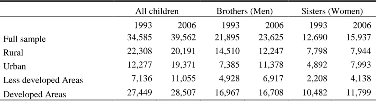
in Table 1. The samples for all children consist of 34,585 observations in 1992/93 and 39,562 observations in 2006. The average numbers of children per family are 2.35 in 1992/93 and 1.98 in 2006. The shares of singleton families in our sample of 16 to 27 years olds are 25 percent in 1992/93 and 36 percent in 2006. More than a third of the families have two children in both survey years.
About 63 percent and 59 percent of our total samples are brothers in 1992/93 and 2006 respectively.
As reported in Table 1, sample sizes for different sub-samples are considerable, the smallest sample size being 2208 for sisters in less-developed states in 1992/93. The large sample sizes ensure precision of our estimates of sibling and intergenerational correlations for both survey years.
Summary statistics from our main samples are presented in Table 2. The education levels of both boys and girls improved between 1992/93 and 2006. Average education of boys increased from 7.63 years in 1992/93 and 8.76 years in 2006. The gains in girls‘ education were more dramatic: it increased from 6.9 years in 1992/92 to 8.67 in 2006. As a result, the gap between boys and girls has narrowed considerably between these two survey years.
27A similar trend can be detected in mother and father‘s education as well though the gender gap in the parent‘s generation remained substantial.
Average education of father increased from 5.33 years to 6.43 years between the two survey years, while that of mother increased from 2.63 years to 3.75 years. The improvements in years of education were associated with a decline in the standard deviation of education levels between the survey years. Consistent with international evidence in Hertz et al. (2009), the variances of education levels are higher in parent‘s generation compared with the kids in both the survey years. This decline in variance implies that relying on intergenerational regression coefficient to understand intergenerational mobility may be misleading.
The summary statistics for the rural sample are also reported in Table 2. As expected, average education levels are lower in rural areas compared with our full sample. Consistent with national trends, average years of schooling have increased for both boys and girls in rural areas. The gender gap in education has also narrowed though the gap is still larger in rural areas compared with our full sample. Summary statistics for other sub-samples also confirm improvements in education attainment of children during this period. The trends in education levels reported here are consistent with those reported in other studies (ASER reports, World Bank (2011)).
In addition to education levels, Table 2 provides summary statistics for age and caste and religion composition of our sample. Overall, the samples from two years appear to be comparable to each other in terms of age and caste-religion composition.
27
Similar convergence in educational attainment between boys and girls over the reform period is observed in China
(see, for example, Behrman et al. (2008)).
15 (4) Empirical Results
Equations (6) and (7) form the basis of empirical estimation of sibling and intergenerational correlations respectively. To estimate the individual and family components of equation (6), we followed the two-step procedure suggested by Bjorklund et al. (2011).
28Unless otherwise noted, all standard errors are clustered at the family level. All sibling pairs are given equal weights in all estimation results presented in this paper.
(4.1) Results from the Full Sample
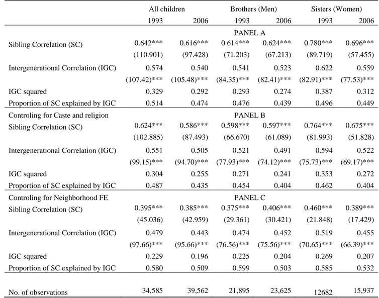
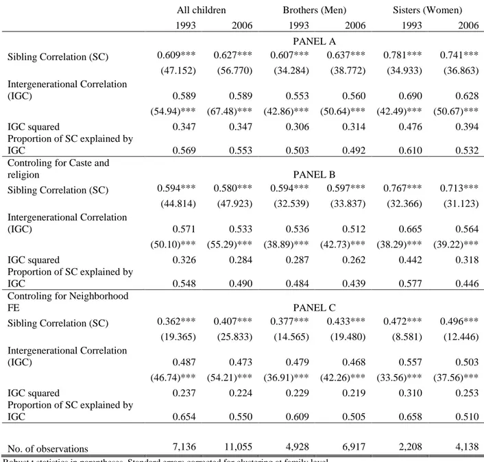
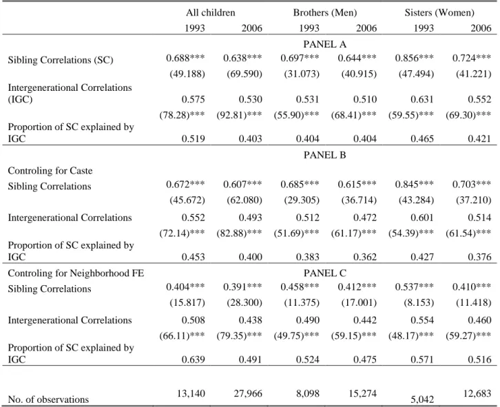
Table 3 reports the results for the full sample. The sibling and intergenerational correlations estimated from our simplest specification of equations (6) and (7) are reported in panel A. In this simplest specification, age dummies are introduced to control for children‘s age, and in the ‗all children sample‘, a female dummy to account for gender difference in education level. The sibling correlation is estimated to be 0.642 in 1993 which declines slightly to 0.616 in 2006. Both of these parameters are estimated with great precision (t-statistics greater than 95). The estimates imply that the influence of the factors common to siblings on their educational attainment is very high (more than 60 percent) and has remained remarkably stable over more than a decade. Interpreting it from a different angle, the estimates of sibling correlations suggest that individual effort and other idiosyncratic factors account for less than 40 percent of variations in schooling years, both in 1992/93 and 2006. The absolute magnitude of the sibling correlation in 2006 is quite high, higher than the available estimates for Latin American countries including Brazil and El Salvador.
29The third row in Table 3 reports the estimates of the intergenerational correlations between children and parents in education. We define the parent‘s education variable as the maximum of
28
Equation (6) can be estimated directly (without the two step procedure) using Stata GLLAMM procedure when the set of control variables is small. However, it becomes unmanageable in the case where we introduce
neighborhood fixed effects. For the sake of comparability, we report results from the two step procedure in this paper. The results from single step estimation do not differ from that of two step procedure when applied to specifications that does not include neighborhood level fixed effects.
29
The highest estimate is 0.60 among 16 Latin American countries, for El Salvador (Dahan and Gaviria (2001).
Among developed countries, sibling correlations are found to be highest in USA. The estimates range between 0.6
(Mazumder (2008) for biological siblings in the same household for age cohort born during 1957-1969 and 0.63
(Conley and Glauber(2008) for siblings with same biological mother for age cohort 1958-76). The average estimate
for Nordic and European countries is around 0.4 (see Bjorklund and Salvanes (2010)).
16
father‘s and mother‘s years of schooling. We, however, note that the results and conclusions in this paper are not sensitive to alternative definitions of parental education such as average of mother‘s and father‘s years of schooling. The intergenerational correlations reported in panel A are estimated from a simple specification that controls only for age and gender. The estimates for all children show a slight decline in intergenerational correlations between two survey years: it declined from 0.574 in 1992/93 to 0.540 in 2006. The absolute magnitude of intergenerational correlation for India is, however, much larger than the average for other Asian countries reported by Hertz et al (2009) (average=0.39).
30Among 10 Asian countries covered by Hertz et al. (2009), only Indonesia has intergenerational correlation in education (0.55) which is comparable to that for India.
31(4.1.1) Gender and Intergenerational Mobility in Education
To understand any possible gender bias in the intergenerational educational mobility, we report estimates of sibling correlations for brothers and sisters separately in columns 3 to 6 of Table 3. The estimates show that while the sibling correlation among men (brothers) did not change perceptibly between 1992/93 and 2006, it experienced a moderate decline in the case of women (sisters). The estimated sibling correlations are: 0.614 (1992/93) and 0.624 (2006) for men and 0.780 (1992/93) and 0.696 (2006) for women. Compared with men, the magnitude of sibling correlation among women is thus significantly higher in both survey years. This is in contrast with evidence from developed countries where there is no significant gender differences in sibling correlations (Bjorklund and Salvanes (2010)). Despite the moderate decline from 1992/93, the estimate for women in 2006 (0.696) is well above the upper bound estimates for sibling correlations among women found in developed and Latin American countries.
32We also analyze the trend in intergenerational correlations between parents and children across gender (columns 3-6, Table 3). The intergenerational correlations for men remained stable (0.541 in 1992/93 and 0.523 in 2006), but for women, it declined moderately from 0.622 to 0.559 between the two survey years, 1993 and 2006. Consistent with our findings regarding sibling
30
While intergenerational correlations for India are estimated for 16-27 age cohorts, the estimates in Hertz et al are for adults in age range 20-69 years. As noted by Hertz et al (2009), with increase in the level of education for younger cohorts, the intergenerational correlations for younger cohorts have either become smaller or not change at all. In that sense, our estimates for the intergenerational correlations for India are likely to be on the conservative side.
31
The intergenerational correlations in Latin American countries are higher than that of India. The average for 7 Latin American countries in Hertz et al (2009) is 0.60.
32
The estimates of sibling correlation among sisters for developed countries fall within the range [0.46-0.6]. Only
one study reported a significant difference in sibling correlations between brothers and sisters for USA (Conley and
Glauber (2008)).
17
correlations, intergenerational correlations are stronger for women than men in both the years. The higher intergenerational persistence observed for women compared with men in India is consistent with the recent findings on intergenerational economic mobility from other developing countries. For instance, Emran and Shilpi (2011) find occupational immobility (as measured by correlations between parents and children) to be much higher for women in Nepal and Vietnam.
As discussed in the conceptual framework above, the square of intergenerational correlation provides an estimate of the share of total variance in schooling that can be explained by parent‘s education alone. The estimates (5
throw in Table 3) show that parent‘s education alone can explain between 27 to 29 percent of variations in years of education for men (brothers) and 31 to 39 percent variations for women (sisters). In contrast, for developed countries, parental education explains only 10 to 20 percent of total variations in schooling years (see Bjorklund and Salvanes (2010)).
(4.1.2) Role of Caste and Religion
A potentially important determinant of educational attainment in India is the caste and religious identity of a household. Studies on education in India show that the average level of education is much lower among children from socially disadvantaged scheduled caste (SC) and scheduled tribes (ST) (Jalan and Murgai (2008), Kajima and Lanjouw (2006), Aslam et al. (2011)).
In the next specification of our regressions, we include dummies for SC, ST and other backward castes. We also include a dummy for households whose head is a Muslim, as Muslim are among the most economically lagging groups in India (Sachar Committee (2006), World Bank (2011)). The effects of the caste and religion dummies on the estimated sibling correlation is minimal; the estimates in panel B of Table 3 are only slightly smaller compared with those reported in panel A.
The inclusion of caste and religion dummies also does not affect the magnitudes of intergenerational
correlations in any significant way. The results thus suggest that sibling and intergenerational
correlations do not vary across caste groups in any significant way in both of the survey years, 1993
and 2006. This is consistent with the findings in Hantskovska et al. (2011) which reported a
convergence of intergenerational persistence in education across castes during last three decades in
India. The conclusion that the sibling and intergenerational correlations do not depend in any
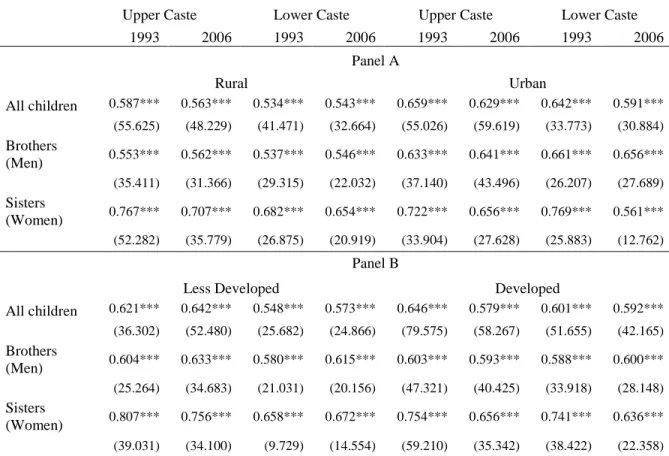
significant way on caste or religious identity is also supported by the estimates from the sub-samples
based on caste and religion. The only exception is the urban women, where lower caste women
experienced significantly higher mobility compared to the upper caste women (see section 4.2.3
below).
18
(4.1.3) Role of Geographic Location: Neighborhood Effect
As noted in the introduction, a focus of this study is to analyze the potential spatial aspects of intergenerational educational mobility in India, and whether the role of geography has changed over time in the post-reform period. A simple but powerful way to gauge the importance of geographic location is to include neighborhood fixed effects in the estimating equations, and then compare the estimates of sibling correlations and intergenerational correlations with and without the neighborhood fixed effect. Note that the fixed effect captures all the factors shared by the children growing up in a neighborhood which include peer effects and school availability and quality, among other things.
Panel C of Table 3 presents the estimates that include neighborhood fixed effects where neighborhood is defined as the sample cluster (PSU). Our full samples include 3799 and 3400 such clusters (PSUs) in 2006 and 1993 respectively. The results show that geographic location as measured by PSU level fixed effect matters a lot for intergenerational mobility in education. The estimates for sibling correlations become substantially smaller when neighborhood fixed effects are taken into account: the sibling correlations in the full sample decline from 0.642 to 0.395 in 1992/93 and from 0.616 to 0.385 in 2006. The implied neighborhood correlations (after netting out caste and gender effects) are 0.23 in 1993 and 0.20 in 2006 for the full sample, 0.22 (1993) and 0.19 (2006) for men, and 0.30 (1993) and 0.29 (2006) for women. These estimates of neighborhood correlations are substantially larger than those found for developed countries (Bjorklund and Salvanes (2010)).
33The neighborhood correlations account for nearly a third of sibling correlations among men and 40 percent of that among women. This can be interpreted as strong evidence in favor of geographic location as a first order mediating factor for the influence of family background on education of children.
34The estimates of sibling correlations in panel C of Table 3 can be considered to be lower bound estimates of family background‘s influence on children‘s educational outcomes (net of caste and religion, and neighborhood effects), because the estimates of neighborhood effects are biased upward due to sorting of similar families in a neighborhood. These lower bound estimates imply that about 40 percent of variations in children‘s education can be explained by family background (net of neighborhood, caste and religion) alone. For women, the net influence of family background declined
33
The largest estimate for neighborhood correlation is 0.15 for USA (Solon et al. (2000)).
34
The relatively larger role of location for women probably reflects lower geographic mobility among them.
19
from 0.46 to 0.39 between 1992/93 and 2006, whereas it increased slightly for men from 0.38 to 0.41 over the same period.
The inclusion of neighborhood fixed effects reduces the estimates of intergenerational correlations between parents and children also. But compared with sibling correlations, the magnitudes of the reductions are much smaller. For instance, estimates for men (brothers) declined from 0.52 to 0.48 in 1992/93 and 0.49 to 0.45 in 2006. After controlling for the neighborhood fixed effects, the estimates of intergenerational correlations indicate that more than 20 percent of variations in total schooling of children and nearly a third of sibling correlations in education can be explained by parent‘s education alone.
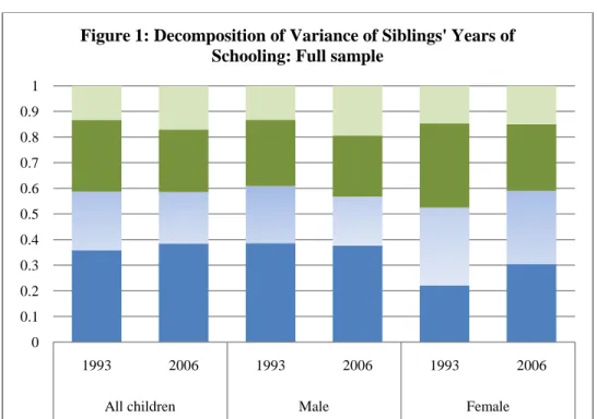
To provide a sense of relative importance of different factors in explaining the variations in children‘s education, we use estimates from Table 3 and plot them in Figure 1. Figure 1 show that in 2006, individual effort and other idiosyncratic factors explain about 40 percent of variations in education outcomes of men, and about 30 percent for women, the rest are due to common factors experienced by siblings. The sibling correlation can be decomposed into three components: (i) parental education, (ii) geographic location (i.e., neighborhood effect), and a residual family environment shared by siblings which presumably capture the parental child rearing skills, among other things. The neighborhood effect and parent‘s education together can explain more than 70 percent of sibling correlations. The common neighborhood factors and parental education are particularly important for sisters (women): their share in sibling correlations is large -- 0.81 in 1992/93 and 0.78 in 2006. For men, contribution of these two factors to sibling correlations decreased from 0.78 in 1992/93 to 0.69 in 2006 due mainly to decrease in the neighborhood correlations (Figure1). For women, intergenerational persistence has declined but neighborhood correlations remain nearly unchanged.
(4.2) Geography of Educational Mobility: Evidence from Alternative Partitioning of the Data
The evidence on strong neighborhood effects in sibling and intergenerational correlations
discussed above brings the focus on geographic location as an important factor in understanding
educational mobility in post-reform India. This raises the question whether the levels, time trends
and gender patterns of sibling and intergenerational correlations differ significantly across different
geographic areas; for example, are there any significant differences between rural and urban areas,
between less developed and more developed states? The recent academic literature and reports in
popular press in India give a strong impression that the rural areas and certain lagging states such as
20
Bihar and Uttar Pradesh (UP) have been largely bypassed by the positive effects of economic liberalization and strong economic growth that followed (World Bank (2011)). In this subsection, we provide additional analysis of the role of geographic location in intergenerational educational mobility.
(4.2.1) Rural vs. Urban Areas
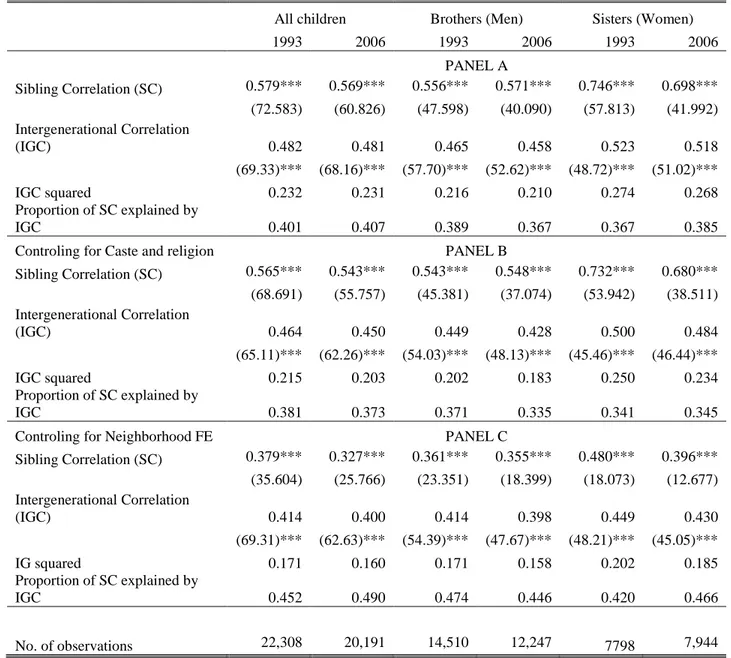
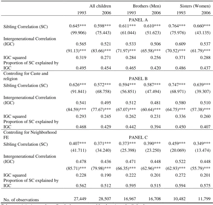
This section presents results from estimation of sibling and intergenerational correlations for families living in rural and urban areas separately. The estimates of sibling and intergenerational correlations for rural and urban areas are reported in Tables 4 and 5 respectively. Consistent with the format of Table 3, we represent estimates from three different specifications of equations (6) and (7) in three panels (A, B and C) of Table 4 and 5. These specifications correspond exactly to the specifications in Table 3 and are not discussed here again for the sake of brevity.
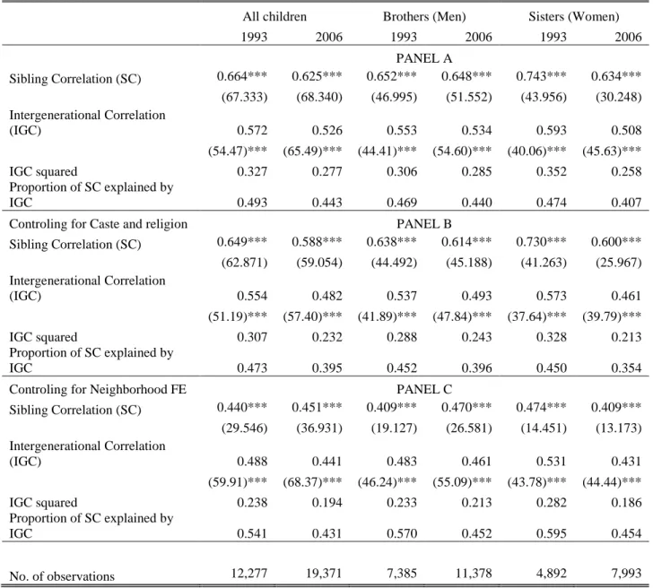
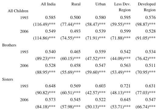
The sibling and intergenerational correlations for all children and for men are larger in magnitudes in urban areas compared with rural areas (Tables 4 and 5). For instance, for all children (men), the sibling correlation is 0.579 (0.556) in rural areas compared with 0.664 (0.652) in urban areas in 1992/93. The corresponding intergenerational correlations are 0.482 (0.465) and 0.572 (0.553) in rural and urban areas respectively. For women in 1992/93, there is practically no difference in sibling correlations between urban and rural areas (both approximately=0.74), though intergenerational correlation is higher in urban areas (0.593 vs. 0.523). Between 1992/93 and 2006, intergenerational correlations remained nearly unchanged for both men and women in rural areas.
There was a marginal decline in the sibling correlation for rural women in the same period, but the sibling correlation among rural men increased slightly. For men in urban areas, both sibling and intergenerational correlations remained effectively unchanged between 1992/93 and 2006. In contrast, sibling and intergenerational correlations have decreased significantly for urban women during the same period. As a result, gender difference in sibling and intergenerational correlations effectively vanished in urban areas, though it is still significant in rural areas.
Using estimates from Tables 4 and 5, we decompose the total variance in children‘s education into individual and common ‗family background‘ components. The family background component is further decomposed into three separate parts accounted for by parental education, common neighborhood environment and other common family factors. The relative contributions of these different factors to total variance of children‘s education are plotted in Figures 2 and 3.
Consistent with results from full sample, influences of parent‘s education and common neighborhood
21
factors are important in both rural and urban areas, accounting for more than 60 percent of sibling correlations for men and 65 percent for women. The contribution of common neighborhood factors to variance in education is larger for rural women whereas parental education is relatively more important for both men and women in urban areas. Overall, common family backgrounds are perhaps most important factor for rural women for whom less than 30 percent of variations in education can be explained by individual effort, choices and other unobserved idiosyncratic factors.
To summarize, though the influences of parental education and common family background are smaller in magnitude in rural areas, there has been little or no progress in mobility in education.
The largest improvement in educational mobility has been experienced by urban women while men experienced effectively no improvement regardless of their location. We find common neighborhood environment and parental education as the most important source of sibling correlations in both urban and rural areas. The influences of common neighborhood factors are particularly important for rural women.
(4.2.2) Less Developed vs. Developed Regions
Living standards in India vary widely across states. The incidence of poverty among poorer states in India is amongst the highest among developing countries. On the other side of the spectrum, many states such as Punjab have low poverty rates that are comparable to richer countries (e.g.
Turkey) (World Bank (2011)). The NFHS 1992/93 identifies the ―backward‖ districts.
35The NFHS 2006 does not identify any district because of confidentiality considerations with respect to AID/HIV testing results. The states where the most backward districts are located can be matched between the two surveys. The backward districts in 1992/93 are located in five states: Bihar, Madhya Pradesh, Rajasthan, Uttar Pradesh and West Bengal. These states are among the poorest in terms of income in 1993/94 (four of them belong to the so-called BIMARU), and also suffer from poor educational attainment and infrastructure indicators (Kingdon (2007), Deaton and Dreze (2002)).
36We take the
35
The Ministry of Health and Family Welfare, Government of India, has defined backward districts as those having a crude birth rate of 39 per 1,000 population or higher, estimated on the basis of data from the 1981 Population Census.
36