Time-Triggered Automotive Software

(1)

BAMBERGER BEITR¨AGE

ZUR WIRTSCHAFTSINFORMATIK UND ANGEWANDTEN INFORMATIK ISSN 0937-3349

Nr. 103

Optimized Buffering of

Time-Triggered Automotive Software

Eugene Yip ・ Erjola Lalo ・ Gerald Lüttgen ・ Michael Deubzer ・ Andreas Sailer

September 2018

URN: urn:nbn:de:bvb:473-opus4-529175 DOI: https://doi.org/10.20378/irbo-52917

FAKULT¨AT WIRTSCHAFTSINFORMATIK UND ANGEWANDTE INFORMATIK OTTO-FRIEDRICH-UNIVERSIT¨AT BAMBERG

(2)

tomorrow's software technologies

Lehrstuhl Softwaretechnik & Programmiersprachen Fakultät Wirtschaftsinformatik & Angewandte Informatik

Optimized Buﬀering for Time-Triggered Automotive Software

^⇤

Eugene Yip,¹ Erjola Lalo,² Gerald Lüttgen,¹ Michael Deubzer,² Andreas Sailer²

1Otto-Friedrich-Universität Bamberg, 96045 Bamberg, Germany

2Vector Informatik GmbH, Franz-Mayer-Str. 1, 93053 Regensburg, Germany

September 21, 2018

Abstract: The development of an automotive system involves the integration of many real-time software functionalities, and it is of utmost importance to guarantee strict timing requirements.

However, the recent trend towards multi-core architectures poses significant challenges for the timely transfer of signals between processor cores so as to not violate data consistency.

We have studied and adapted an existing buffering mecha- nism to work specifically for statically scheduled time-triggered systems, called static buffering protocol. We developed further buffering optimisation algorithms and heuristics, to reduce the memory consumption, processor utilisation, and end-to-end response times of time-triggered AUTOSAR designs on multi-core platforms. Our contributions are important because they enable deterministic time-triggered implementations to become competitive alternatives to their inherently non-deterministic event- triggered counterparts. We have prototyped a selection of optimisations in an industrial tool and evaluated them on realistic industrial automotive benchmarks.

⇤Research support was provided by the Bayerische Forschungsstiftung under grant no. AZ-1257-16, project OBZAS.

(3)

Technical Report Contents

1 Introduction

The development of an automotive system involves the integration [OSHK09] of many real- time software functionalities, where it is critical to guarantee strict timing requirements.

The automotive open system architecture (AUTOSAR) standard [AUT17a] is popular for developing modular software components with high interoperability. An important type of requirement, calledend-to-end response time, specifies the maximum time that the system can take to deliver an output to a corresponding input. Such timing requirements are easier to guarantee with time-triggered implementations because they oﬀer better time- predictability than their event-triggered counterparts [Kop91]. However, the recent trend towards multi-core architectures poses significant challenges for the timely transfer of data and control signals between processor cores so as not to violate data consistency.

In this light, the automotive industry [EKQS18, HvHM⁺16, RNH⁺15] has shown great interest in using the logical execution time (LET) task model [KS12] for designing time- triggered multi-core systems. A LET task has a statically defined period and block of time, called thelogical execution time, during which the task is allowed to execute its computations. Task communication via signals is limited to the start and end of each LET, and is idealised to complete in zero time. This ensures time-predictable and deterministic communication that is unaﬀected by changes in the underlying platform [HK07]. This platform invariant property is attractive to automotive manufacturers as it greatly simplifies the migration of legacy single-core software to multi-core platforms [HvHM⁺16, RNH⁺15].

The automotive industry is also taking advantage of LET tasks as design contracts between control and software engineers, and between component suppliers and system integra- tors [EKQS18]. However, signal buffering is needed to preserve the data- and control-flow between the tasks [FNG⁺09], especially when their LETs do not align. Thus, significant time may be spent on managing the buffers, and significant memory may be needed for the buffers [FNG⁺09].

1.1 Contributions

Despite the increasing interest in the LET time-triggered approach, event-triggered systems remain popular because of their ability to achieve better average-case response times and resource utilisation [Kop91]. To improve the practicality of the time-triggered approach, we present an adaptation of thedynamic buffering protocol (DBP) [STC06] that is suitable for LET communication, and develop buffering optimisation algorithms and heuristics to reduce the memory consumption, processor utilisation, and end-to-end response times for multi-core time-triggered AUTOSAR designs. The algorithms and heuristics synthesise the required buffers and associated accesses for each signal, and the mapping of tasks to processor cores.

When adapting existing buﬀering protocols to LET tasks, attention is needed to the fact that LET communication is defined to occur instantaneously at predefined time points. Our contributions are important to allow time-triggered implementations to become competitive alternatives to their event-triggered counterparts.

1.2 Report structure and Content

Section2recalls (1) the AUTOSAR methodology for developing automotive systems, (2) the scheduling of LET tasks, and (3) the challenges with implementing a system that preserves the LET semantics. Section 3 discusses related work on buﬀering protocols developed for real-time task communication. We find that DBP is a good candidate for buﬀering LET communication. Section4presents related work on algorithms and heuristics developed for

(6)

Technical Report 1 Introduction

optimising AUTOSAR designs, focussing on the execution time and memory cost of task communication and on end-to-end response times.

Section 5 discusses the heterogeneous hardware and software architecture that is assumed, followed by an overview of our proposed buﬀering optimisation approach in Section6.

Our approach consists of optimisations that are applied during the design and deployment of an LET system. The overall optimisation goal is to reduce processor and memory utilisation due to task communication, and to reduce end-to-end response times. The design phase optimisations (see Section 7) include the adaptation of DBP to statically scheduled LET tasks (calledstatic buffering protocol, SBP), and the suppression of unnecessary signal writes. Our optimisations support signals to which multiple task write, and signals that may be assigned several values before stabilising on a final value. The deployment phase optimisations (see Section 8) formulate the assignment of signal buffers-to-memory mod- ules, of tasks-to-cores, and of buffering protocols to each signal as a mixed-integer linear programming (MILP) problem. Because solving resource allocation problems is NP-hard, a genetic algorithm of the MILP problem is provided for situations where possibly suboptimal solutions are acceptable for faster solving time. Once memory allocations are found for the signal buffers, a heuristic is used to merge buffers with disjoint lifetimes.

We evaluated a selection of the proposed optimisations on synthetic benchmarks, based on actual airbag, chassis, and engine management systems, and on an industrial engine management system from the FMTV Challenge [HDK⁺17]. Section 9 describes the implementation of the selected optimisations in the TA Tool Suite [Vec18], which aids AUTOSAR designers in modelling, designing, and analysing the timing behaviour of event-triggered or time-triggered multi-core automotive software. Sections 10 and 11 explain the setup of the synthetic and industrial benchmarks, respectively, and discuss preliminary results that suggest that LET-based AUTOSAR designs with SBP require less memory and execution time than with the traditional point-to-point communication approach. Finally, Section 12 provides concluding remarks on the optimisation of LET communication in AUTOSAR designs.

(7)

Technical Report 2 Background

Virtual Function Bus

SWC 0 r0 r1 r2

SWC 1 r3 r4 r5

r₀

r1

r₂ r₃ r₄ r5

r1 r2

r1

r2

r0

s₀

s₁ o0

i0

s1

s₀

Core 0 OSEK OS t₀ r₀ t₁ r₁ t₂ r₂

Core 1 OSEK OS t₃ r₃ t₄ r₄ r₅ Memory 0

(Local to Core 0)

Memory 1 (Local to Core 1)

Bus (Round-robin, fixed-priority, or first-come first-served arbitration)

Memory 2

1 void r0(void) { 2 if (s0 < 0) { 3 return -s0; 4 } else {

5 return s0; 6 }

7 }

-9 10 Value

of s₀ 10 is read

-9 is read Partial value is read

LET

Initial task offset

Activation offset

Period

Time (LET start)

Read inputs (LET end)

Write outputs

WCET

New value for s₀ is being written

s₀ Time

0 1

r₂ s₁

0 1

t0

0 2 4

Time (ms)

t₁ 0

1 3

2 4

1 3

t0

t₁ s0 s1

s0 s1 s0 s1

(a) Design phase (ris a runnable).

Memory 1 (Local to

Core 1)

Bus (Round-robin, fixed-priority, or first-come first-served arbitration)

Memory 2

1 void r

0

Initial task offset

Activation offset

Period

Time (LET start)

Read inputs (LET end)

Write outputs

WCET

New value for s

0

is being written

s

₀

Time

0 1

r

₂

s

₁

0 1

t

₀

0 2 4

Time (ms)

t

₁

0 1 3

Memory 1 (Local to

Core 1)

Bus (Round-robin, fixed-priority, or first-come first-served arbitration)

Memory 2

1 void r

₀

Initial task offset

Activation offset

Period

Time (LET start)

Read inputs (LET end)

Write outputs

WCET

New value for s

₀

is being written

s

(c) Event-chainec0, with in- puti0 and outputo0. Virtual Function Bus

SWC 0 r₀ r₁ r₂

SWC 1 r₃ r₄ r₅

r₀ r1

r₂ r₃ r₄ r₅ r₁ r₂

r₁ r₂ r₀ s₀

s₁ o₀ i0

s1

s₀

Core 0 AUTOSAR OS t₀ r₀ t₁ r₁ t₂ r₂

Core 1 AUTOSAR OS t₃ r₃ t₄ r₄ r₅ Memory 0

(Local to Core 0)

Memory 2

1 void r0(void) { 2 if (s0 < 0) { 3 return -s0; 4 } else { 5 return s0; 6 }

7 }

-9 10 Value

of s0

10 is read

LET

Initial task offset

Activation offset

Period

Time (LET start)

Write outputs

WCET

New value for s0

is being written

s₀ Time

0 1

r₂ s₁

0 1

t₀

0 2 4

Time (ms)

t₁ 0

1 3

2 4

1 3

t₀

t1

s₀ s₁

s₀ s₁ s₀ s₁

(d) Deployment phase (t is a task).

Figure 1: AUTOSAR methodology.

2 Background

This section discusses the challenges surrounding the deployment of AUTOSAR designs onto multi-core platforms. Of note is the need to ensure data consistency among communicating tasks, and the desire to maintain time-predictable behaviour among the possible platform configurations.

2.1 AUTOSAR Methodology

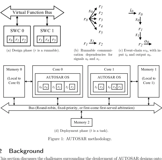
An AUTOSAR design [AUT17a] consists of one or more self-contained software components (SWCs) that communicate over memory-mapped signals. A software component contains one or more so-called runnables that each encapsulate the smallest code-fragment that can be scheduled by an operating system. Figure 1a exemplifies a small design with two SWCs and six runnables. Runnables communicate over signals, and Figure 1bshows some dependencies for the signals s0 and s1. For signal s0, runnable r0 is the sole writer and runnables r1 to r5 are the readers. For signals1, runnable r1 is the writer and runnable r2

is the reader. Communication dependencies influence the execution order of the runnables, and cyclic dependencies are broken by delaying one of the communication links.

When deploying an AUTOSAR design, runnables are mapped to operating system tasks.

Due to resource constraints, AUTOSAR-compliant operating systems typically only support a limited number of tasks and several runnables may be mapped to the same task. The 6 of 76

(8)

Technical Report 2 Background Virtual Function Bus

SWC 0 r0 r1 r2

SWC 1 r3 r4 r5

r₀ r1

r₂ r₃ r4

r₅ r₁ r₂

r1

r₂ r0

s₀

s₁ o₀ i0

s₁ s0

Core 0 AUTOSAR OS t₀ r₀ t₁ r₁ t₂ r₂

Core 1 AUTOSAR OS t₃ r₃ t₄ r₄ r₅ Memory 0

(Local to Core 0)

Memory 2

1 void r0(void) { 2 if (s0 < 0) { 3 return -s0; 4 } else { 5 return s0; 6 }

7 }

-9 10 Value

of s0

10 is read

LET

Initial task offset

Activation offset

Period

Time (LET start)

Write outputs

WCET

New value for s₀ is being written

s0 Time

0 1

r2

s1

0 1

t₀

0 2 4

Time (ms)

t1

0

1 3

2 4

1 3

t₀

t1

s0 s1

s₀ s1 s₀ s1

Figure 2: Example of signal stability and partial reading issues.

mapping also depends on whether a runnable contains specific computations that can only be executed or accelerated by a particular type of processor core (e.g., floating point or digital signal processing operations) or needs to access specific peripherals for sensing or actuating.

In such a case, several runnables from diﬀerent SWCs may need to be mapped to the same task to be executed by a specific core. Figure 1d shows a possible multi-core deployment of Figure1a. It is common for an input signal to be processed by a sequence of runnables, and an event-chain [KKTM10] can be used to capture the causal relationships between event occurrences. The event-chain ec₀ of Figure 1c defines that input i₀ is processed by runnables r0, r1, and r2 to produce output o0, with intermediate signals s0 and s1 being produced along the way. The time that an event-chain needs to generate an output from its input is its end-to-end response-time. Data age constraints [AUT17c], such as r0

s0,

! r1, can be specified to enforce that the value ofs₀ read by r₁ must not have been written byr₀ more than time units ago.

After mapping the tasks to a multi-core platform, a scheduling discipline is selected to manage the sharing of resources (e.g., memory and processor time) among the tasks. Incor- rect values may be communicated between tasks if insufficient time is given to complete the communications, or insufficient (buffer) memory is allocated. In such cases, the implementation is incorrect and must be rectified, e.g., by redesigning the software or by provisioning more resources. Static timing analysis [WEE⁺08] is typically performed to validate the real-time behaviour of the system before it is placed into operation.

2.2 Preemptive Task Scheduling and Data Consistency

AUTOSAR [AUT17a] defines the use ofAUTOSAR OS as the basis for fixed-priority preemptive task scheduling [LL73] to preferentially execute higher priority tasks for shorter response times. When a higher priority task is activated, e.g., by a periodic timer, the scheduler interrupts the executing task and begins to execute the higher priority task. The scheduler saves the execution context of the preempted task so that its execution can be resumed later, after all the higher priority tasks have completed their executions. Preemp- tion can cause non-deterministic timing behaviours, because task interruptions depend on their priorities and actual execution times. This results in end-to-end response times with high jitter, which is undesirable for real-time automotive systems.

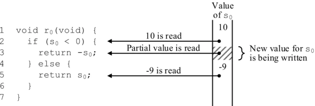
Preemptive scheduling can cause signal writes and reads to interleave among the tasks, leading to inconsistent values being read. For example, in Figure 2, runnable r0’s code for returning the absolute value of signals0 is shown on the left side, and s0’s value over time is shown along the right side. The runnable begins by reading the value 10 for s0, which is a positive number. It attempts to return the original value ofs0, which is updated to 9in the meantime. Hence, an incorrect value is returned because s0’s value wasunstable duringr0’s

(9)

execution. If instead s0’s value is read while it is updated (e.g., line 3 in Figure 2), then only a partial value is read. Signal stability and partial reading issues can cause runnables to branch along incorrect paths or to compute incorrect values for other signals.

When a task needs to read from multiple signals, it is possible that some of the signals are tightly coupled, e.g., the sampling of an engine’s temperature and rotational speed as two periodic signals. A task reads such tightly coupled signals in a coherent manner if it reads the n-th value of each signal together. In any real implementation, it takes time to deliver sensor values to the tasks. Hence, the system must be robust against delays because they can cause tasks to read diﬀerent signal instances together (incoherent reads). It is the responsibility of the system designer to define the coherent signals. We only address the concerns for data stability and the prevention of partial reads by using appropriate data protection mechanisms. Signal coherency builds on top of signal stability and would require signal instances to be tracked at run-time. We consider signal coherency as future work.

2.3 Data Protection Mechanisms

Data protection mechanisms [HZN⁺14, Ray13, BCB⁺08], e.g., locks, are needed to give tasks exclusive access to signals. However, the use of locks in real-time multi-core systems is undesirable [HZN⁺14] because they can cause parallel tasks to block and sequentialise their executions, to suﬀer from deadlocks, and to experience priority inversions where higher priority tasks are blocked by lower priority tasks. Thus, locks introduce additional inter- core interferences that are complex to analyse [GGL14].

Lock-free methods [Her90] attempt to minimise the blocking time by allowing tasks to access signals without locks. An access is successful if no other task has updated the signal at the same time. Otherwise, the access must be retried until successful. The number of retries can be bounded [Her90] to estimate the worst-case access time. It should be noted that lock-free methods solve the partial read issue, but do not provide signal stability.

Wait-free methods [Her90] provide a strategy that is based on keeping snapshots of a signal’s value from different points of time, and tasks access specific snapshots stored in buffers. This enables tasks to access signals independently and concurrently without having to block or retry, making wait-free methods amenable to static timing analysis. Once a snapshot is no longer needed by any task, its buffer element can be reused for a new snapshot.

Since a signal’s value in a snapshot is constant, signal stability can be guaranteed. Compared to locks and lock-free methods, wait-free methods provide short predictable access times and signal stability, but may require significant buﬀer memory to be allocated. Section3reviews a selection of wait-free methods developed for real-time systems.

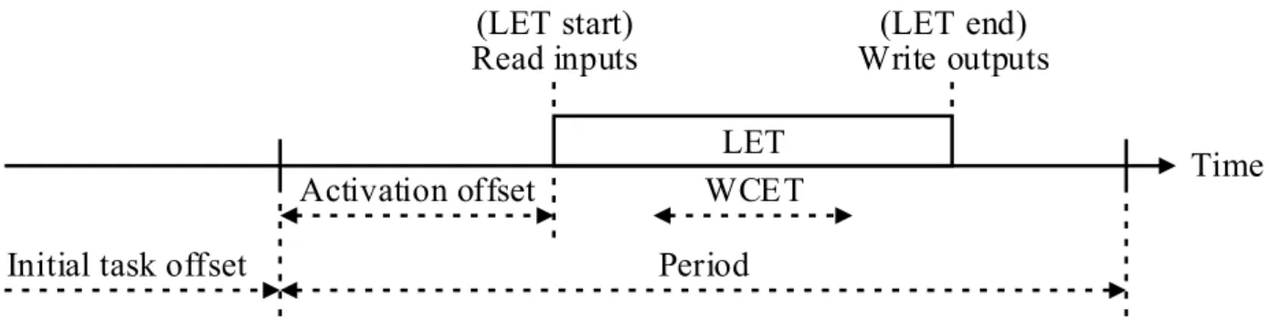
2.4 Logical Execution Time (LET) Task Model

The LET task model [KS12] was originally developed as part of the time-triggered Giotto language [HHK01]. It is being used by the automotive industry to enhance legacy em- bedded control software with real-time behaviour [RNH⁺15] and to parallelise their execution [HvHM⁺16]. Figure 3 illustrates the parameters of a LET task: the period contains a block of time, called the logical execution time (LET), during which the task can execute its computations for up to its worst-case execution time (WCET). If the task fails to complete before the end of its LET, i.e., the task’s deadline, then a timing error occurs and it must be handled by the run-time (e.g., by dropping the task instance). The start of the LET is determined by an activation oﬀset, which can be zero. All tasks start their first period together when the system is initialised. A positive initial task oﬀset can be specified to

(10)

Technical Report 2 Background Virtual Function Bus

SWC 1 r1 r2 r3

SWC 2 r4 r5 r6

r1

r2

r3

r4

r5

r6

r2 r3

r2

r3

r1

s1

s2

o1

i1

s2

s1

Core 1 OSEK OS t1 r1 t2 r2 t3 r3

Core 2 OSEK OS t4 r4 t5 r5 r6

Memory 3

1 void r1(void) { 2 if (s1 < 0) { 3 return -s1; 4 } else {

5 return s1; 6 }

7 }

-9 10 Value

of s₁ 10 is read

LET

Initial task offset

Activation offset

Period

Time (LET start)

Write outputs

WCET

New value for s₁ is being written

s1 Time

1 2

r3

s2

1 2

t1

0 2 4

Time (ms)

t2

0

1 3

2 4

1 3

t1

t2

s1 s2

s1 s2 s1 s2

Figure 3: Parameters of a LET task.

delay the start of the task’s first period. The end of a task’s period coincides with the start of its next period. The following constraints can be used to validate a task’s parameters:

• period activation oﬀset+LET: Ensures that the period is long enough to contain the LET;

• LET WCET: Ensures that the LET provides enough time to execute the task’s computations.

The task reads its input signals at the start of its LET and their values remain constant throughout the LET. The task writes its output signals at the end of its LET. The writing and reading of signals at the LET boundaries is idealised to occur instantaneously in zero time, thus guaranteeing by design that signal values are updated atomically and remain sta- ble during task execution. Because task communication only occurs at the LET boundaries, the task’s input/output behaviour is time-predicable and decoupled from the task’s computation time. Although this greatly simplifies the static analysis of end-to-end response times, it also imposes an artificial delay on signal communication, which the implementation must preserve.

2.5 Static Scheduling of LET Tasks

AUTOSAR [AUT17a] defines the use of schedule tables (for each core) to implement time- triggered systems. A schedule table defines a sequence of task activations to be performed at predefined times, and can be constructed using the base-period [YKRB14] or hyper- period [YKRB14,CM05] approach. In the base-period approach, time is divided into equally sized slots, called the base-period, in which tasks are allocated some time to execute their computations. As a result, tasks are executed preemptively in a time-sliced manner. Its main advantage is the ability to reuse the slack that builds up at the end of each base- period, so as to support variable task periods [YKRB14]. However, scheduling overheads become significant when the base-period is much shorter than the task periods. The hyper- period approach constructs longer schedules that contain consecutive instances of each task.

The hyper-period approach allows for better schedulability than the base-period approach, because computations can be scheduled over the entire task period, such that unnecessary time-slicing preemptions are avoided.

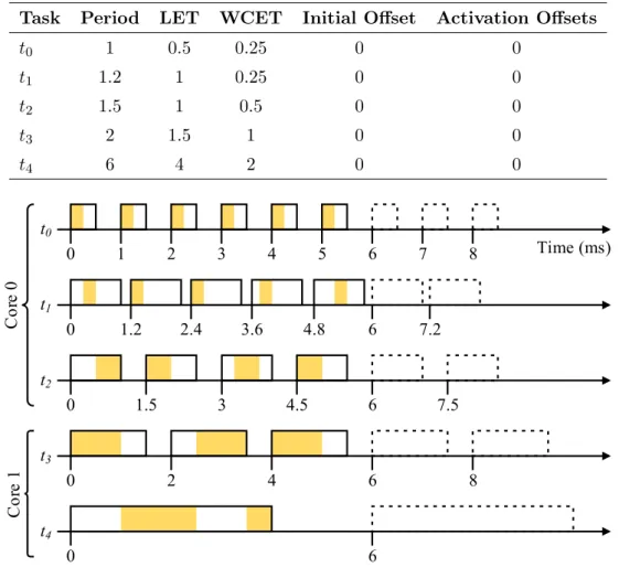
For this work, LET tasks are statically scheduled using the hyper-period approach because support for variable task periods is not needed. Figure 4shows a 6 mshyper-period schedule for the tasks in Table 1. The first step in constructing a hyper-period schedule is to allocate the WCET of each task (shaded segments in Figure 4) within the LET of their initial period. Subsequent task instances are appended to the schedule until all tasks end

(11)

Technical Report 2 Background Table 1: Example timing information (in ms) for the tasks in Figure 1d

Task Period LET WCET Initial Oﬀset Activation Oﬀsets

t₀ 1 0.5 0.25 0 0

t₁ 1.2 1 0.25 0 0

t₂ 1.5 1 0.5 0 0

t₃ 2 1.5 1 0 0

t4 6 4 2 0 0

t₀

0 1 2 3 4 5 6 7 8

t1

0 1.2 2.4 3.6 4.8 6 7.2

t₂

0 1.5 3 4.5 6 7.5

t3

0 2 4 6 8

t₄

0 6

t₀ 1

0 1 2 3 4 5 6

2 3 4 5 6

t₁ 0

0 1.2 2.4 3.6 4.8 6

1 2 4 5

t₂ 0

0 1.5 3 4.5 6

2 3 5

t₃ 0

0 2 4 6

2 4

t4 0

0 6

0 ? ? ?

Buffer’s contents:

Writer’s pointers:

Readers: ^t¹^,t²^, t3,t4

0 1 ? ? next, prev Buffer’s contents:

Readers: t1,t2, t3,t4

0 1 2 ? Buffer’s contents:

Readers: t4

Buffer’s initial state (0 ms)

Buffer’s state at 2 ms

t1 t2,t3

Buffer’s state at 0.5 ms

Time (ms)

Time (ms) Core 0Core 1

t0 1

0 1 2 3 4 5

2 3 4 5 Time

t0 (ms)

t₁ s0

t₁ 1 2 4

0 1.5 3 4.5

t0 1

0 1 2 3 4 5

2 3 4 5 Time

(ms)

1 2 4

t_w 1

0 2 4

2 Time

(ms)

tr 0 1

Reader and Writer needs input and output buffering

t_w

0

0 2 4

1

Time (ms)

tr

1 2

Writer needs output buffering

0 1.5 3 4.5

Buffer elements e0e1e2

?

? 0

e3 ?

0p

?n 1

? p

? n 2

p n 3

p

?n 4 p ?

n 5 p ?

n 6 p

Figure 4: Hyper-period schedule of6msfor the tasks in Table1. Execution times allocated in each LET are indicated by shaded segments.

their last period together. Thus, the duration of the resulting hyper-period schedule is equal to the least common multiple (LCM) of the task periods. At run-time, if the boundaries of multiple LETs occur together, then the writes always precede the reads. This ensures that the latest value of each signal can be read.

System schedulability is demonstrated by constructing a hyper-period schedule that provides enough time for tasks to execute at their WCET during their LET. The guarantee of signal stability and the absence of partial reads by the LET semantics allow tasks to be scheduled preemptively for improved schedulability [KS12]. A LET in the hyper-period schedule contains slack if it is not completely allocated to execute tasks. For Core 1 in Figure 4, task t3’s third LET contains slack. Note that there is no slack in t3’s first two LETs and int₄’s first LET because those time periods are allocated completely to executet₃ and t4. If every LET contains slack, then the system’s end-to-end response times can be reduced by scaling down the timing parameters of all tasks until a task no longer has any slack. This results in a shorter hyper-period. However, absolute timing behaviour is not preserved by this approach.

2.6 Preservation of LET Communication Semantics

One key benefit of using the LET task model is that its formal semantics [HHK01] facilitates the formal verification [CW96] of a system’s functionality and timing behaviour against its 10 of 76

(12)

requirements. An implementation that preserves the LET semantics does not need to be verified, since its behaviour would be identical to that of the original design. When given the same sequence of (timestamped) inputs, a semantics preserving implementation and its original design would produce the same sequence of (timestamped) outputs, i.e., the data-flow and its timing are preserved. However, the idealised instantaneous writing and reading of signals at LET boundaries cannot be realised by any implementation; time is always needed. Thus, a correct implementation must ensure that suﬃcient time is provided to access signals so as to preserve the original data-flow and its timing.

2.7 Use of LET as a Design Contract

The automotive industry is actively exploring [EKQS18] the use of the LET task model as a design contract between control engineers, who demand information on the delays that their control loop could experience, and software engineers, who are responsible for implementing the control algorithms such that they run at their designed rate. The control and software engineers would negotiate on how the control algorithm is to be mapped as sequences of runnables to LET tasks, and on the LET timing characteristics. The mapping has to consider the resource needs of each runnable, which may be restricted to specific processor cores, e.g., signal processing execution units, or peripherals for sensing and actuating. Once the contract is settled, the control and software engineers could start working independently of each other. The control engineers would design their algorithm, knowing the expected end-to-end response times of the final implementation with high confidence. The software engineers could explore different implementation options with minimal risk in affecting the control quality. Consequently, it is undesirable to later modify the runnable-to-task map- pings, because the end-to-end response times may be greatly affected, warranting a full redesign of the control algorithm.

(13)

Technical Report 3 Related Work on Semantics Preserving Buﬀering Table 2: Categorisation of the semantics preserving protocols reviewed in Section 3

Centralised:

Dynamic buﬀering protocol (DBP) [STC06]

Temporal concurrency control protocol (TCCP) [WNSV07]

Timed implicit communication protocol (TICP) [KQBS15]

Decentralised:

AUTOSAR implicit communication [AUT17a]

LET point-to-point (PTP) buﬀering [RNL17,HvHM⁺16,RNH⁺15]

3 Related Work on Semantics Preserving Buﬀering

This section reviews the wait-free buffering protocols that have been proposed for AU- TOSAR task communication [AUT17a], and for time-triggered communication based on LET semantics [KS12] and the closely related synchronous-reactive semantics [BCE⁺03]. A buffering protocol defines the necessary actions that the run-time and tasks need to take to manage and access a buffer’s content. The protocol guarantees that the signal writer and readers always access the same buffer elements at disjoint times, and that the freshest value is always read. Typically, a buffer is created for each signal and its value is written by the output of a dedicated task, called the writer of the signal. A task that reads the signal’s value as input is called a reader of the signal. Note that a task can write to or read from multiple signals.

Table 2categorises buﬀering protocols as beingcentralised [KQBS15,WNSV07,STC06]

ordecentralised [RNL17, HvHM⁺16,AUT17a,RNH⁺15] depending on the buffer’s location in memory. Centralised protocols use a buffer that is located in global memory. With decentralised protocols, a signal’s value is written to the writer’s local buffer, and the readers are responsible for copying the value into their own local buffers. Although centralised protocols can be more memory efficient than decentralised protocols, accessing global buffers can be more time consuming for frequent signal accesses.

3.1 AUTOSAR Implicit Communication

AUTOSAR supports the decentralised buﬀering of signals via so called implicit communication [AUT17b]. For each runnable, the AUTOSAR run-time environment copies its input signals into local variables before the runnable is executed, and writes its output signals after the runnable has terminated. Runnables access their own copy of inputs during execution. Thus, signal stability and the absence of partial reads is guaranteed by the run-time.

However, even on the same platform, the run-time does not guarantee the timing or ordering in which the inputs and outputs are copied. Hence, implicit communication is inherently non-deterministic and, thus, unsuitable for preserving LET semantics.

3.2 LET Point-to-Point (PTP) Buﬀering

Buﬀering protocols proposed for LET systems are based on a decentralised point-to-point (PTP) approach [RNL17, HvHM⁺16, RNH⁺15]. These protocols are designed for systems that use priority-based task scheduling, such as OSEK OS [OSE05]. A task’s output signal is computed and stored in a local buﬀer, and only made available at the end of its LET.

When a reader of the signal starts its LET, it stores a copy of the signal in its own local buﬀer. Thus, the collective buﬀer size for a signal is equal to R+ 1, where R is the number

(14)

Technical Report 3 Related Work on Semantics Preserving Buﬀering Table 3: Example timing information (inms) from Table1 for the tasks in Figure 1d

Task Period WCET

t₀ 1 0.25

t₁ 1.2 0.25

t₂ 1.5 0.5

t₃ 2 1

t4 6 2

of readers and “1” is needed for the writer, although this can be reduced by performing buffer analysis [RNL17, RNH⁺15] to identify the tasks that do not require buffering for semantics preservation. The analysis also identifies tasks that can share a global buffer without affecting the communication behaviour, resulting in a more centralised protocol.

3.3 Dynamic Buﬀering Protocol (DBP)

In contrast to LET tasks, where outputs are expected at predefined times, the outputs of synchronous-reactive tasks [BCE⁺03] are assumed to be produced instantaneously (in zero time) when inputs arrive. However, in any real implementation, tasks need time to compute their outputs. In addition, a task’s computation time can vary from one instance to another. Thus, buﬀering is needed to ensure that tasks read from the correct output instances [NWV08,STC06] in order to preserve the synchronous communication semantics.

Sofronis et al. [STC06] propose adynamic buffering protocol (DBP) that is memory optimal in the sense that only the output instances needed for semantics preservation are buffered, with no assumptions made on task activation or completion times. The writing task uses a next pointer to track the buffer element that will hold the new value being computed, and a prev pointer to track the buffer element of its previously computed output. Each time the writing task is activated, it assigns next to prev, and an algorithm is executed to find a free buffer element that is not used by a reading task or pointed to by prev. The next pointer is updated to point to the free buffer element. When a reading task is activated (at the start of its period), it copies the address held in next. This address specifies the buffer element that the reading task uses throughout its computation. The address held in previs copied instead if the reading task has a higher priority than the writing task. Buffer elements are freed and reused when their values are no longer needed by the readers.

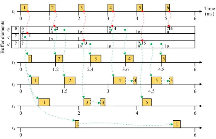
Figure 5 demonstrates DBP for signal s₀ from Figure 1b, using the task periods and WCETs from Table 3 (i.e., treating them as ordinary tasks without LET semantics). The task priorities, in descending order, are t0 > t1 > t2 > t3 > t4. Since DBP is designed for single-core platforms, the execution trace assumes rate-monotonic, preemptive scheduling [LL73] on a single core. At 0 ms, after all tasks have been activated, the readers will read from buffer elemente1, even though its value is currently undefined. By the time the readers are scheduled for execution, t₀ has written the value 1 into buffer element e₁. We see that buffer element e1 could not be reused duringt4’s entire period. At 2ms, the buffer is fully utilised because element e0 holds the previous value, element e1 is being read by taskt₄, and elemente₂ is needed for the writer’s next value that task t₃ reads. Even after t₂ is preempted at 4.8 ms, it continues to correctly read value 5, instead of the next value 6 computed byt0.

DBP can be configured to store up tok previous values of a signal, which is useful when tasks need a sliding window of values for signal processing [BDM02], or need to access pre-

(15)

Technical Report 3 Related Work on Semantics Preserving Buﬀering

0p

?n

? 1

?n p

2

n 3 p

p

?n 4

?n p

5

?n

p 6

t0

t0 1

0 1 2 3

2 3

t1 1

0 1.2 2.4 3.6 4.8 6

2 3 4 5

t2 1

0 1.5 3 4.5 6

2 4 5

t3 1

0 2 4 6

3 5

t4 1

0 6

Time (ms)

4 5

1

4 5 6

5

4 6

3

0 ? ?

Readers: ^t1,t2, t3,t4

Buffer’s state at 0 ms after all tasks have been activated

0 1 ?

Readers: t3,t4

Buffer’s state at 0.8 ms during t3

2 1 ?

Readers: t4

Buffer’s state at 2 ms after t0 and t3 have been activated

t3

t0

Buffer elements e0e1e2

?

? 0

Figure 5: Example execution of the tasks in Table3using DBP for signals0 from Figure1b.

For the first6ms, the contents of signal s0’s buffer are displayed below the writert0. Each buffer element is shown as a row, containing its value (“?” if the value is being computed) and whether it is being referenced by the writer’s next (n) or prev (p) pointer. Changes to a buffer element’s value or to the writer’s pointer references are demarcated by solid vertical lines. Writes and reads are drawn as dotted arrows going into and out of the buffer, respectively. The values written and read by the tasks are shown inside their respective LETs. Task preemptions are indicated by dotted vertical lines.

14 of 76

(16)

Technical Report 3 Related Work on Semantics Preserving Buﬀering

vious values to correctly implement software pipelining [MRR12]. Moreover, DBP supports the over- and under-sampling of signals when tasks of diﬀerent periods communicate. Un- der dynamic task scheduling, a lower bound for a signal’s buﬀer size is calculated [STC06]

as Rlp+k + 1, where Rlp is the number of lower priority readers, and k is the number of previous values to retain. For Figure5, a buﬀer size of4would be calculated, although only a size of 3is actually needed.

3.4 Temporal Concurrency Control Protocol (TCCP)

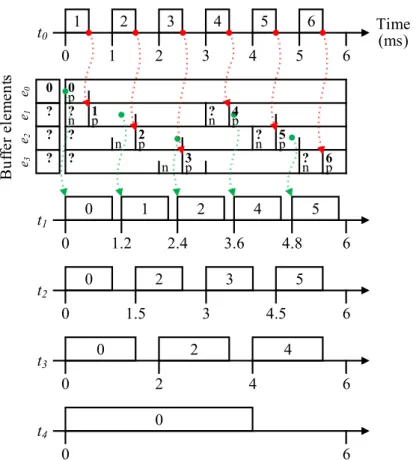
Wang et al. [WNSV10, WNSV07] provide several OSEK-compliant implementations for DBP and analyse their costs in terms of required memory and execution time, given in Table 4. The main decider for the required memory and execution time is the algorithm for finding a free buffer element. For the constant-time implementation, an auxiliary linked list is used to track the free buffer elements, leading to a higher memory requirement than the linear-time implementation, which simply iterates through the entire buffer until a free element is found. Wang et al. [WNSV10, WNSV07] also describe a temporal concurrency control protocol (TCCP) that uses a circular buffer [KR93] to store a signal’s values in consecutive (chronological) order. Thus, finding a free buffer element only involves incre- mentingnext to point to the next buffer element. For TCCP, the buffer size is bounded by the number of writes that could occur during the longest task period among the readers. If TCCP had been used for Figure5, then a buffer size of 7 would be calculated.

3.5 Timed Implicit Communication Protocol (TICP)

The timed implicit communication protocol (TICP) [KQBS15] extends AUTOSAR implicit communication by tagging each written value with a monotonically increasing timestamp.

To preserve the communication semantics, each reader is responsible for finding the value with the correct timestamp. In any real implementation, the memory for storing each timestamp is bounded, posing a limit on the system’s run-time before a timestamp overflow occurs [ST00]. No algorithms are suggested to find a free buﬀer element for the writer, to find the correct timestamped values for the readers, or to handle bounded timestamps.

TICP appears to be similar to DBP, except that DBP implicitly maintains the necessary timestamp information with the prev and next pointers.

3.6 Related Buﬀering Protocols

Other buffering protocols have been proposed, but are not directly applicable to LET communication. First in, first out (FIFO) buffering [Hab72] is used in point-to-point signal communication, where a reader needs to receive all values computed by a writer. The reader consumes (reads and then clears) the oldest value in the buffer. However, FIFO buffering is unsuitable when tasks have different periods, because it can lead to buffer over- or under-flow. Similar to FIFO buffering is lossless [YKRB14] and synchronous data flow (SDF) buffering [LM87]. In lossless buffering, the reader consumes all values in the buffer each time it is activated. In SDF buffering, each time a task is activated, it consumes or writes a fixed number of values into the buffer. We do not consider SDF or lossless buffering in this work because current automotive systems do not require such communication behaviour.

(17)

Technical Report 3 Related Work on Semantics Preserving Buﬀering Table 4: Memory and execution time costs for DBP, TCCP, and PTP, where B is the number of buﬀer elements, R is the number of readers, Rlp is the number of lower priority readers, k is the number of previous values to retain, p^max_R is the maximum task period among the readers, andp^min_W is the minimum task period of the writer

Memory Time to find buffer element Buffering protocol Buffer Auxiliary for writing for reading Linear-time DBP [WNSV07]

B=Rlp+k+ 1 3R+B+ 2 O(B)

Constant-time DBP [WNSV07] 3R+B+ 3 O(1) Constant-time TCCP [WNSV07] O(1)

⇠p^max_R +p^min_W p^min_W

⇡

+k 2R+ 2

Constant-time PTP [RNH⁺15] R+ 1 0

3.7 Discussion

The memory and time trade-oﬀ highlighted by Table 4 is that a faster buﬀering protocol needs to store more information about the tasks at run-time, while a slower protocol needs time to reconstruct the information every time it is invoked. The semantics preserving DBP, TCCP, and TICP protocols have been designed with priority-based, preemptive task scheduling in mind, and make no assumptions about task activation and completion times.

Moreover, they assume that a signal has only one writer, whereas real automotive software can have signals with multiple writers. Only task periods are required, which are used to derive task priorities. Therefore, buffer management algorithms need to be executed at run-time, e.g., to find a free buffer element for the writer, and to find the correct signal snapshot to read. These buffering protocols assume a more general task model than LET, and can be adapted to preserve LET semantics. However, by design, DBP and TCCP are limited to single-core platforms, because tasks are assumed to execute sequentially and never in parallel. By observing that LET tasks have precisely defined input reading and output writing times, their computation and buffer accesses can be statically scheduled so as to avoid the need to manage the buffers at run-time. Moreover, exact buffer sizes can be computed for each signal by inspecting the static schedule (see Section7.1).

It should be noted that the actual buffer size needed by DBP is never greater than that of TCCP [STC06]. However, depending on the task periods, the calculation of a lower bound on the buffer size needed by DBP can sometimes be worse than that of TCCP, leading to the over-provisioning of buffer memory. Natale et al. [NWV08] reduce the calculated lower bounds for DBP by observing that readers, with slightly longer periods than the writer’s period, access the same subset of buffer elements. Thus, the reading tasks are partitioned into faster tasks and slower tasks, and a lower bound is calculated for each set. The lower bounds are summed together to obtain a final lower bound. For Figure 5, an improved buffer size of3 would be calculated, equal to what is actually needed.