Lecture 10: Estimation
1 State Estimation
In the previous chapters, we assumed that all the state variables of a given systen system were available at each time. In real systems, however, this is not the case: one knows just the output y(t) and the input u(t). Hence, one has to figure out how to get the actual state x(t). The idea is to use an observer to get an estimate of x(t), also called ˆx(t).
A whole course about estimation if offered at IDSC in the master by Prof. D’Andrea:
Recursive Estimation.
1.1 Preliminary Definitions
Definition 1. A system is said to be observable if for any time T > 0 it is possible to determine the state of the systemx(T)∈Rn through the measurements ofu(t) and y(t), with t ∈[0, T].
A pair (A, C) is observable if and only if rank(O) =n = dim(A), where
O=
C CA
... CAn−1
(1.1)
is the observability matrix.
Definition 2. A pair (A, C) is detectable if all the unobservable modes are stable.
Definition 3. A linear system is reachable if for any x0, xf ∈ Rn, there exists a T > 0 and u(t) : [0, T]→Rsuch that the corresponding solution satisfiesx(0) =x0 and x(T) = xf ∈Rn.
Reachability test: A system (A, B) is reachable if and only if rank(R) = n, where x∈Rn and
R= B AB . . . An−1B
. (1.2)
Remark. Note that for continuous linear time invariant systems, controllability is the same as reachability. In general, reachability implies controllability, but not the converse.
1.2 Problem Definition
Given a linear, time invariant system
˙
x(t) = Ax(t) +Bu(t)
y(t) = Cx(t) +Du(t), (1.3)
at each time instant t construct an estimate of the state ˆx(t) by only measuring the system’s inputs and outputs, such that
t→∞lim(x(t)−x(t)) = 0.ˆ (1.4)
1.3 The Luenberger Observer
In order to do this, one creates a numerical copy of the system (an observer)
˙ˆ
x(t) = Aˆx(t) +Bu(t) ˆ
y(t) = Cˆx(t) +Du(t), (1.5)
and one observes the dynamics of the estimation error ˆ
e=x(t)−x(t).ˆ (1.6)
It holds
˙ˆ
e(t) = ˙x(t)−x(t)˙ˆ
=Ax(t) +Bu(t)−Aˆx(t)−Bu(t)
=Aˆe(t).
(1.7)
If matrix A has all the eigenvalues in the left half-plane, the error ˆe(t) will converge to zero, resulting in a correct state estimation. But is this what we want? Essentially, our error is converging to zero because the states of the two systems are designed to converge to zero. In particular, we are not using the output as an information. How can we solve the problem even for unstable systems? For the following, consider the structure reported in Figure 1. Let’s add feedback from the measured output by considering the observer
˙ˆ
x(t) = Aˆx(t) +Bu+L(y(t)−y(t)).ˆ (1.8) It holds
˙ˆ
e(t) = ˙x(t)−x(t)˙ˆ
=Ax(t) +Bu(t)−Aˆx(t)−Bu(t)−L(y(t)−y(t))ˆ
=Ax(t)−Ax(t)ˆ −L(Cx(t)−Cx(t))ˆ
= (A−LC)ˆe(t).
(1.9)
With this new equation, one can choose a matrix L such that the matrix A−LC has eigenvalues with negative real parts and hence such that the error ˆe(t) will converge to 0.
This observer is known as the Luenberger observer.
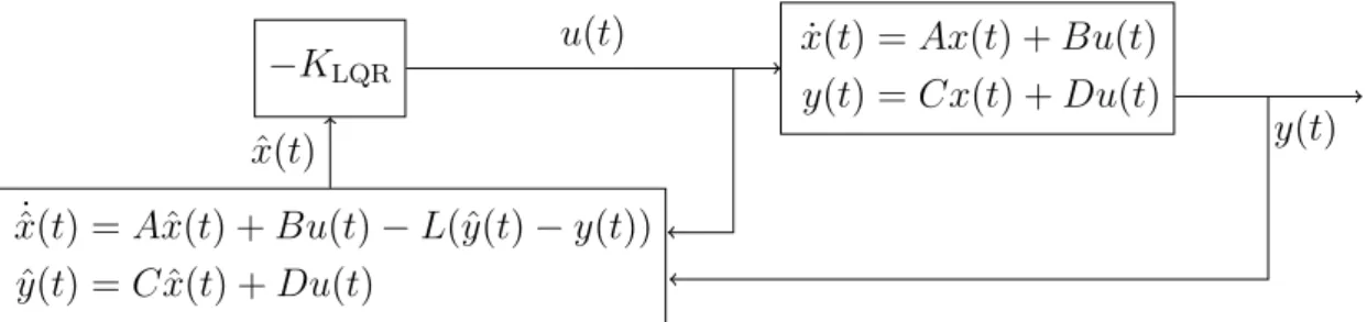
˙
x(t) =Ax(t) +Bu(t) y(t) =Cx(t) +Du(t)
˙ˆ
x(t) =Aˆx(t) +Bu(t) +L(y(t)−y(t))ˆ y(t) =ˆ Cx(t) +ˆ Du(t)
u(t) x(t)
ˆ
x(t) y(t)ˆ −
y(t)
Figure 1: Luenberger Observer
1.3.1 Duality of Estimation and Control
The structure of Equation 1.9 is similar to the one of state feedback we introduce in the previous chapter. Considering the state feedback dynamic equation
˙
x(t) = (A−BK)x(t), (1.10)
one can find in Equation 1.9 some analogies. In particular, it holds
˙ˆ
e(t) = ( A|
|{z}
A˜
− C|
|{z}
B˜
L|
|{z}
K˜
)|e(t).ˆ (1.11)
Since the problem has the same form, one can use the same methodology to solve it.
One recalls that pole placement is allowed if and only if the system is reachable, i.e. if rank(R) = n = dim(A), where R is the reachability matrix defined in Equation 1.2 By using the analogies, one can define similarly
R˜ = B˜ A˜B . . .˜ A˜n−1B˜
= C| A|C| . . . (A|)n−1C|
=
C CA
... CAn−1
|
=O|,
(1.12)
where O is the observability matrix defined in Equation 1.1. Using the well known rule
rank(O) = rank(O|), (1.13)
one can impose rank(O) to be n in order for observer pole placement to be feasible.
Starting from the Ackermann formula for state feedback K = 0 . . . 1
R−1p∗cl(A), (1.14)
one can write
K˜ =L|
= 0 . . . 0 1R˜−1p∗cl(A)
⇒L=p∗cl(A)O−1 0 . . . 0 1|
.
(1.15)
1.3.2 Putting Things Together
Considering Figure 2, one can define the augmented state
˜ x(t) =
x(t) ˆ e(t)
. (1.16)
The dynamics read
˙˜
x(t) = x(t)˙
˙ˆ e(t)
=
A−BK BK
0 A−LC
| {z }
Acl
x(t) ˆ e(t)
(1.17)
Since Acl is upper triangular, it holds
σ(Acl) =σ(A−BK)∪σ(A−LC). (1.18) This is known as the separation principle. Intuitively, this means that control and esti- mation do not interact with each other, hence can designed independently.
−KLQR x(t) =˙ Ax(t) +Bu(t) y(t) = Cx(t) +Du(t)
˙ˆ
x(t) =Aˆx(t) +Bu(t)−L(ˆy(t)−y(t)) ˆ
y(t) =Cx(t) +ˆ Du(t)
u(t) ˆ y(t)
x(t)
Figure 2: Observer Problem: Closed loop system.
In general one follows this procedure:
1. Design the controller first. FindK to place the poles of A−BK where you desire in the LHP.
2. Design the observer. Find Lto place the poles of A−LC in the LHP. As a rule of thumb, make the observer 10 times faster than the controller.
1.4 Linear Quadratic Gaussian (LQG) Control
LQR relies on the assumption that the states are known. How can one integrate the defined estimation procedure in the LQR framework? Is the optimality defined for the LQR method affected by this? In the following, we recall the LQR problem definition and its solution.
1.4.1 LQR Problem Definition
With LQR one wants to find a stabilizing input uLQR(t), t∈[0,∞] such that uLQR(t) = argmin
u
Z ∞ 0
u(t)|Ru(t) +x(t)|Qx(t) + 2x(t)|N u(t)dt (1.19) satisfying
• the dynamics
˙
x(t) =Ax(t) +Bu(t), x(0) =x0 (1.20) and
z(t) = Ex(t) +F u(t), (1.21) with u(t)∈Rm×1, z ∈Rk×1 and x∈Rn×1.
• Q >0,R >0, Q=Q|,R =R|, with
R=F|QF¯ +ρR,¯ ρ∈R+ Q=E|QE¯
N =E|QF.¯
(1.22)
1.4.2 LQR Problem Solution If
1. The system (A, B) is stabilizable and
2. the pair ( ˜A,Q) = (A˜ −BR−1N|, Q−N R−1N|) is detectable, then
uLQR(t) =−R−1(N+P B)|
| {z }
KLQR
x(t), (1.23)
whereP is the real, symmetric, positive definite solution of the algebraic Riccati equation (ARE)
(A−BR−1N|)|
| {z }
A¯|
P +P (A−BR−1N|)
| {z }
A¯
+P (−BR−1B|)
| {z }
R¯
P + (Q−N R−1N|)
| {z }
Q¯
= 0 (1.24)
1.4.3 Simplified Case
It turns out that choosing N = 0 results in nice robustness properties. By writing P∞ instead of P (we are solving the finit horizon), one can simplify the ARE as
A|P∞+P∞A−P∞BR−1B|P∞+Q= 0. (1.25) 1.4.4 Stady-state Kalman Filter
The observer problem, i.e. find L in
˙ˆ
x(t) =Aˆx(t) +Bu(t) +L(y(t)−y(t))ˆ (1.26) such that (A−LC) is stable, shows duality with the control problem, i.e.
C|→B, A|→A, L|→K. (1.27)
Thank to this duality, one can solve the estimation problem by solving the control one.
The algebraic Riccati equation for estimation is
AP∞+P∞A|−P∞C|R−1CP∞+Q= 0. (1.28) The matrix L can be found with
L|=R−1CP∞⇒L=P∞C|R−1. (1.29) The duality exists also for the technical conditions for the ARE:
(A|, C|) stabilizable ↔(A, C) detectable .
(A|, Q) detectable ↔(A, Q) stabilizable. (1.30)
Deterministic Interpretation
It is worth mentioning that the Kalman filter’s theory is not that short. Among others, stochastic interpretation, recursive formulatiom, finite horizon and discrete time imple- mentation represent important topics to be discussed. However, for the aim of this course, we use the deterministic interpretation of Kalman filters. Considering the effect of dis- turbances/noises on the plant
˙
x(t) =Ax(t) +Bu(t) +w(t), x(0) =x0
y(t) =Cx(t) +Du(t) +n(t), (1.31) where w(t) represents the process noise and n(t) the measurement noise. The Kalman Filter can be interpreted deterministically as minimizing an uncertainty measure
kx0k22+ Z T
0
kwk22+knk22dt, (1.32)
i.e. estimating the last energy/most likely initial condition, disturbance and measurement noise that justify the measurements.
1.4.5 Summary
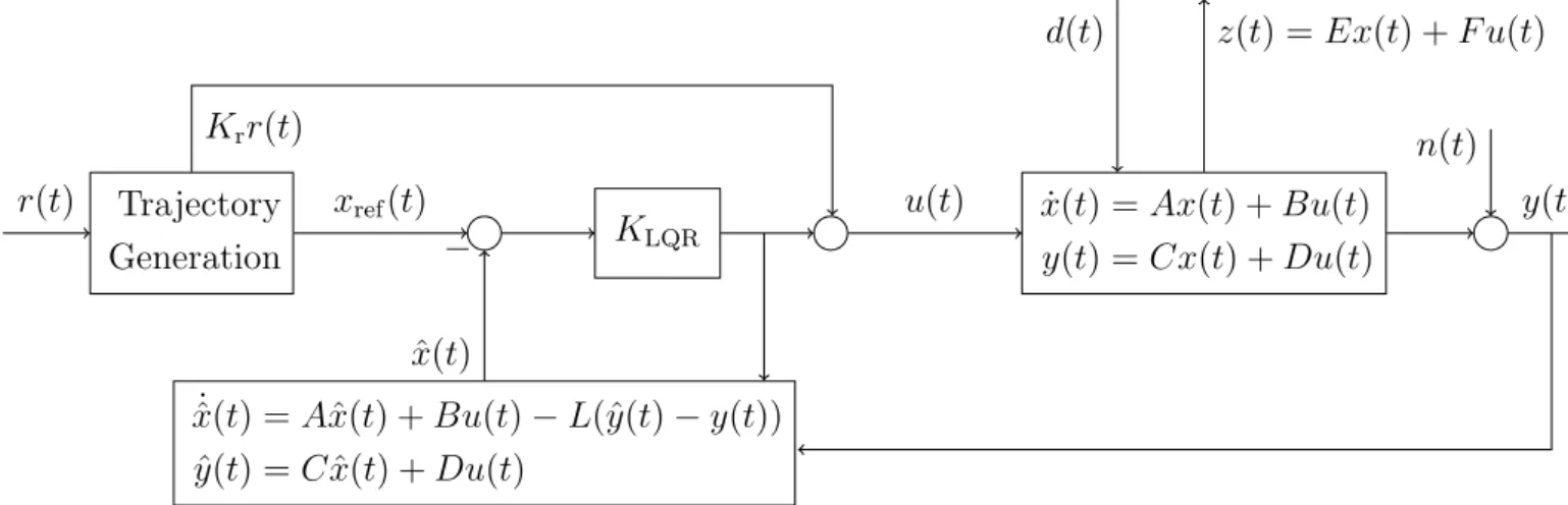
The linear quadratic gaussian (LQG) regulator is the union of a LQR controller and a Kalman Filter. One can see such a closed loop system in Figure 3. The closed loop is
Trajectory
Generation KLQR x(t) =˙ Ax(t) +Bu(t)
y(t) =Cx(t) +Du(t)
˙ˆ
x(t) = Aˆx(t) +Bu(t)−L(ˆy(t)−y(t)) ˆ
y(t) = Cx(t) +ˆ Du(t)
xref(t) u(t)
z(t) =Ex(t) +F u(t) d(t)
n(t)
y(t)
− ˆ x(t) r(t)
Krr(t)
Figure 3: LQG Problem: Closed loop system.
stable if and only if K is a stabilizing state feedback gain andLis a stabilizing estimation gain.
1.5 Examples
Example 1. The dynamics of a system are given as
˙
x1(t) = x2(t)
˙
x2(t) = u(t) y(t) = x1(t).
(1.33)
You want to design a state observer. The observer should use the measurements for y(t) and u(t) in order to estimate the state variables ˆx(t)∼x(t).
(a) Which dimension should the observer matrix L have?
(b) Compute the observer matrix L for R= 1 andQ=BB|.
(c) You have already computed a state feedback matrix K = 1 1
for the system above. What is the complete transfer function of the controller C(s)?
Solution.
(a) Since C∈R1×2 matrix andL·C has the same dimensions ofA∈R2×2,L is a 2×1 matrix, i.e.
L= L1
L2
. (1.34)
(b) First of all, let’s read from 1.33 the system matrices:
A= 0 1
0 0
B = 0
1 C = 1 0 D= 0.
(1.35)
Plugging these matrices into the algebraic Riccati equation and using the unknown matrix
Ψ =
ψ1 ψ2 ψ2 ψ3
, (1.36)
one gets:
1
R ·Ψ·CT ·C·Ψ−Ψ·AT −A·Ψ−B·BT = 0 Ψ·
1 0
· 1 0
·Ψ−Ψ· 0 1
0 0
− 0 0
1 0
·Ψ− 0
1
· 0 1
= 0 0
0 0 ψ12 ψ1·ψ2
ψ1·ψ2 ψ22
−
2ψ2 ψ3
ψ3 0
− 0 0
0 1
= 0 0
0 0
. (1.37) The matrix Ψ is symmetric and positive definite and with these informations we can compute its elements:
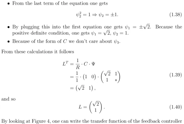
• From the last term of the equation one gets
ψ22 = 1 ⇒ψ2 =±1. (1.38)
• By plugging this into the first equation one gets ψ1 = ±√
2. Because the positive definite condition, one gets ψ1 =√
2,ψ2 = 1.
• Because of the form of C we don’t care about ψ3. From these calculations it follows
LT = 1
R ·C·Ψ
= 1
1 · 1 0
· √
2 1
1 ∗
= √
2 1 ,
(1.39)
and so
L= √
2 1
. (1.40)
(c) By looking at Figure 4, one can write the transfer function of the feedback controller as
Figure 4: Structure of LQG controller.
.
C(s) =ˆ K·(s·I−(A−B·K−L·C))−1 ·L. (1.41) By plugging in the found matrices one gets
(A−B·K−L·C) = 0 1
0 0
− 0
1
· 1 1
− √
2 1
· 1 0
= 0 1
0 0
− 0 0
1 1
− √
2 0
1 0
= −√
2 1
−2 −1
.
(1.42)
It follows
(s·I−(A−B·K −L·C))−1 =
s+√
2 −1 2 s+ 1
−1
= 1
(s+√
2)·(s+ 1) + 2·
s+ 1 1
−2 s+√ 2
. (1.43) By plugging this into the formula one gets
C(s) =ˆ K·(s·I−(A−B·K−L·C))−1·L
= 1 1
· 1
(s+√
2)·(s+ 1) + 2·
s+ 1 1
−2 s+√ 2
· √
2 1
= 1
(s+√
2)·(s+ 1) + 2· s−1 s+ 1 +√ 2
· √
2 1
= 1
(s+√
2)·(s+ 1) + 2·(√
2s−√
2 +s+ 1 +√ 2)
= (√
2 + 1)s+ 1 (s+√
2)·(s+ 1) + 2.
(1.44)
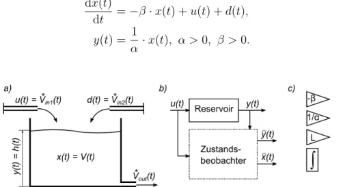
Example 2. You are working for your semester thesis at a project which includes a water reservoir. Your task is to determine the disturbanced(t) that acts on the reservoir. Figure 5 shows the situation. The only state of the system is the water volumex(t) = V(t). The volume flows in the reservoir Vin∗(t) are the known system input u(t) and the unknown disturbance d(t) > 0. The volume flow of the system is assumed to be only dependend on the water volume, i.e.
Vout∗ (t) = −β·x(t). (1.45)
The system output y(t) is the water levelh(t). The model of this reservoir reads dx(t)
dt =−β·x(t) +u(t) +d(t), y(t) = 1
α ·x(t), α >0, β >0.
(1.46)
Figure 5: a) Drawing of the reservoir; b) Inputs and Outputs of the observer; c) Blocks for signal flow diagram.
.
The goal is to determine d(t). Your supervisor has already tried to solve the model equations ford(t): he couldn’t determine the change in volume dx(t)dt with enough precision.
Hence, you want to solve this problem with a state observer.
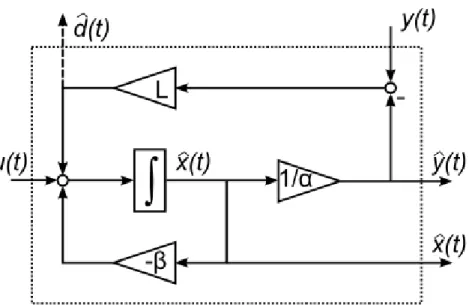
(a) Draw the signal flow diagram of such a state observer. Use the blocks of Figure 5c).
(b) The state feedback matrix L is in this case some scalar value. Which value can L be, in order to get an asymptotically stable state observer?
(c) Introduce a new signal ˆd(t) in the state observer. This should approximate the real disturbance d(t).
(d) Find the state space description of the observer with inputsu(t) andy(t) and output d(t).ˆ
Solution.
(a) The signal flow diagram can be seen in Figure 6.
Figure 6: Signal flow diagram of the state observer.
.
(b) The stability of the ovserver depends on the eigenvalues of A−L·C. In this case, since A−L·C is a scalar,
A−L·C < 0 should hold. This leads to
L > A
C. (1.47)
With the given informations it follows
L >−β
α. (1.48)
(c) The dashed line in Figure 6 represents the new output ˆd(t). The integrator in Figure 6 has now 3 inputs. The arrow from downwards from the reservoir is Vout∗ (t), the arrow from left is the input flow u(t) = Vin1∗ (t). If we simulate the system without the dashed arrow, there is a deviation between the measured y(t) and the simulated ˆ
y(t). This results from the extra inflowd(t) = Vin∗(t), which is not considered in the simulation.
(d) The new state-space description reads dˆx(t)
dt =
−β− L α
·x(t) + (1)ˆ ·u(t) + (L)·y(t) (1.49) d(t) =ˆ
−L α
·x(t) + (0)ˆ ·u(t) + (L)·y(t). (1.50)
References
[1] Essentials of Robust Control, Kemin Zhou.
[2] Karl Johan Amstroem, Richard M. Murray Feedback Systems for Scientists and En- gineers. Princeton University Press, Princeton and Oxford, 2009.
[3] Sigurd Skogestad, Multivariate Feedback Control. John Wiley and Sons, New York, 2001.