Stigma and Social Control

July 2002

Stigma and Social Control

Lawrence Blume

Impressum Author(s):

Lawrence Blume Title:

Stigma and Social Control ISSN: Unspecified

2002 Institut für Höhere Studien - Institute for Advanced Studies (IHS) Josefstädter Straße 39, A-1080 Wien

E-Mail: o ce@ihs.ac.atffi Web: ww w .ihs.ac. a t

All IHS Working Papers are available online: http://irihs. ihs. ac.at/view/ihs_series/

This paper is available for download without charge at:

https://irihs.ihs.ac.at/id/eprint/1443/

Stigma and Social Control

Lawrence Blume

Reihe Ökonomie

Economics Series

119 Reihe Ökonomie Economics Series

Stigma and Social Control

Lawrence Blume July 2002

Institut für Höhere Studien (IHS), Wien

Institute for Advanced Studies, Vienna

Contact:

Lawrence Blume Department of Economics Uris Hall

Cornell University

Ithaca, New York 14850, USA email: lb19@cornell.edu

Founded in 1963 by two prominent Austrians living in exile – the sociologist Paul F. Lazarsfeld and the economist Oskar Morgenstern – with the financial support from the Ford Foundation, the Austrian Federal Ministry of Education and the City of Vienna, the Institute for Advanced Studies (IHS) is the first institution for postgraduate education and research in economics and the social sciences in Austria.

The Economics Series presents research done at the Department of Economics and Finance and aims to share “work in progress” in a timely way before formal publication. As usual, authors bear full responsibility for the content of their contributions.

Das Institut für Höhere Studien (IHS) wurde im Jahr 1963 von zwei prominenten Exilösterreichern – dem Soziologen Paul F. Lazarsfeld und dem Ökonomen Oskar Morgenstern – mit Hilfe der Ford- Stiftung, des Österreichischen Bundesministeriums für Unterricht und der Stadt Wien gegründet und ist somit die erste nachuniversitäre Lehr- und Forschungsstätte für die Sozial- und Wirtschafts - wissenschaften in Österreich. Die Reihe Ökonomie bietet Einblick in die Forschungsarbeit der Abteilung für Ökonomie und Finanzwirtschaft und verfolgt das Ziel, abteilungsinterne Diskussionsbeiträge einer breiteren fachinternen Öffentlichkeit zugänglich zu machen. Die inhaltliche Verantwortung für die veröffentlichten Beiträge liegt bei den Autoren und Autorinnen.

Abstract

Social interactions provide a set of incentives for regulating individual behavior. Chief among these is stigma, the status loss and discrimination that results from the display of stigmatized attributes or behaviors. The stigmatization of behavior is the enforcement mechanism behind social norms. This paper models the incentive effects of stigmatization in the context of undertaking criminal acts. Stigma is a flow cost of uncertain duration which varies negatively with the number of stigmatized individuals. Criminal opportunities arrive randomly and an equilibrium model describes the conditions under which each individual chooses the behavior that, if detected, is stigmatized. The comparative static analysis of stigma costs differs from that of conventional penalties. One surprising result with important policy implications is that stigma costs of long duration will lead to increased crime rates.

Keywords

Crime, stigma, social norms

JEL Classifications

C730, Z130

Comments

I am grateful to the Cowles Foundation for Economic Research, the Department of Economics at Yale University, and the Institute for Advanced Studies in Vienna for very productive visits. I am also grateful for financial support from the John D. and Catherine T. MacArthur Foundation, the Pew Charitable Trusts, and the National Science Foundation. This research is a consequence of several stimulating conversations with Daniel Nagin, and has been helped along by comments from Buz Brock, Tim Conley, Steven Durlauf, Tim Fedderson, Josef Hofbauer, Karla Hoff, Chuck Manski, and Debraj Ray.

Contents

1 Introduction 1

2 The Model 3

3 Individual Choice and Social Equilibrium 5

3.1 States and Strategies ...5

3.2 The Individual’s Decision Problem ...6

3.3 Equilibrium – Existence and Monotone Comparative Statics ...8

3.4 A Discrete Example ... 10

4 The Equilibrium Tagging Process 12

4.2 Equilibrium in the Long Run ... 13

4.3 Tag Duration in the Long Run ... 15

4.4 The Discrete Example: Short Run, Large N ... 16

4.5 The Discrete Example: Long Run, Large N ... 17

5 Conclusion 19 6 Proofs 23

6.2 Theorem 4 ... 32

6.3 Computing Equilibria ... 33

Notes 34

References 36

“. . . , let her cover the mark as she will, the pang of it will be always in her heart.”

The Scarlet Letter Nathaniel Hawthorne

1 Introduction

Consciously or not, in our interactions with others we identify markers that signal particular attributes. While the attribution signalled by a marker may be the result of rational inference, markers may also signal attributes by triggering stereotypes. Language usage, skin color, gender and occupation may all prompt individuals to infer that others possess a variety of behaviors and attitudes that have nothing at all to do with the markers they display.

Markers that trigger negative stereotypes stigmatize their bearers.

The sociology and social psychology literature on stigma is replete with characterizations of the stigmatic process. Link and Phelan’s (2001, p. 367) definition is particularly useful here because it addresses the social as well as the psychological aspects of stigma. They characterize stigma in terms of four interrelated components:

In the first component, people distinguish and label human dif- ferences. In the second, dominant cultural beliefs link labeled persons to undesirable characteristics—to negative stereotypes.

In the third, labeled persons are placed in distinct categories so as to accomplish some degree of separation of “us” from “them”.

In the forth, labeled persons experience status loss and discrimi- nation that leads to unequal outcomes.

Stigma has both micro- and macrosocial consequences. Link and Phelan

(2001) assert that research on stigma has attended primarily to its perception

by individuals and its consequences for micro-level interactions. On the other

hand, stigmatic markers classify entire groups of individuals. The aggregate

of behaviors which respond to stigmatic markers has systemic implications

for aggregate social and economic performance.

Introduction

2 Both individual characteristics and individual behaviors are available for stigmatic representation. The stigmatization of race, gender, physical disabilities, mental illness and other characteristics is morally repugnant, and a continuing source of social ills. But the stigmatization of behaviors is the central mechanism for enforcing social norms. Stigma is thus essential to the production of what some call “social capital”. Stigma enforces social norms by stigmatizing non-normative behavior. Here this mechanism is modeled in order to draw some conclusions about its efficacy. A concrete instance of the social control process modeled here is the stigmatization of certain kinds of criminals. Small-town newspapers routinely publish the names of those arrested (and not yet convicted) for driving under the influence of alcohol.

Fears of public exposure are a strong incentive for tax compliance in some communities. But if everyone cheated or everyone drank, the social costs of exposure would be small.

The stigma mechanism suggests a coordination game, with high- and low-activity equilibria. In the high-activity equilibrium, many people cheat, and so the stigma costs of cheating are small — cheating is not stigmatized.

The low-activity equilibria has few cheaters and high stigma costs — cheaters are stigmatized. But my interest here is in the dynamics of stigma costs rather than in the description of static coordination games. The costs of being stigmatized are born in the future as well as today. Accounting for the future requires the consideration of stigma cost dynamics.

The model presented here is a dynamic population game model, loose-

ly in the spirit of Blume (1993), Kandori, Mailath, and Rob (1993) and Young

(1993). But it departs from these earlier dynamic models in its rejection of

myopia. The usual population model from evolutionary game theory su-

perimposes on a static game some dynamics meant to describe the flow of

the distribution of strategies among the population. The chief drawback to

this conventional modelling strategy is that individuals’ decisions are uncon-

nected to considerations of the future. This is frequently justified by claiming

that individuals are myopic. With infinite subjective rates of time preference

they have no need to consider the future consequences of their acts. The

technical innovation of this paper is developing a population model in which

individuals care about the future and account for the future evolution of the

population in their decisionmaking. A suitable equilibrium concept is intro-

duced and proved to exist. The comparative dynamics of equilibrium with

respect to parameters of the model is worked out. The long-run implica- tions for levels of criminal activity are demonstrated. Finally, a particular example is worked out in some detail, which demonstrates some additional consequences of equilibrium both in the short and in the long run.

2 The Model

Consider the criminal story — the stigmatization of tax cheaters and drunk drivers. The model contains two types of individuals: “Tagged” individuals have been caught and labeled as criminals at some point in the past. They have been stigmatized by having been caught displaying antisocial behav- ior. “Untagged” individuals bear no such label. There is a cost associated with criminal status. The magnitude of this cost is increasing in the size of the untagged population. There is no further stigma cost to additional crime once an individual is tagged. Tagged individuals revert to untagged status at random moments. The stigma of being tagged eventually wears off. This dis- tinguishes crime, occupational choice and other stigmata marked by actions from those marked by characteristic, such as race, gender and mental illness, which may never wear off. Time is continuous and individuals maximize the present discounted value of a utility stream whose magnitude depends upon the following parameters.

Notation:

N The population size.

m

The fraction of “other” untagged individuals.

p The arrival rate of criminal opportunities.

u The (random) utility reward for successfully completing a crime.

v The utility penalty for being apprehended and convicted. δ = u

qv is the expected instantaneous return to committing a crime.

F (u) The cdf of the reward u.

The Model

4 q The probability of being captured and convicted after committing a crime.

(We suppose the corresponding probability conditional on not commit- ting a crime is 0.)

c(m) The stigma (flow) cost of being tagged when the fraction of others who are untagged is m. This function is non-decreasing.

g The arrival rate of untaggings.

r The individual’s instantaneous rate of time preference.

Intuitively, the equilibrium process evolves as follows. At random moments events happen to individuals in the population. Events are either crime opportunities or the removal of a tag (if present). Crime opportunities arrive to a given individual at rate p. When a crime opportunity arrives a return u to committing the criminal act is drawn (independently) from the distribution F . The individual, knowing the state and the return to crime, must decide whether or not to act. If she does not act, she receives 0 return and is not tagged. If she commits the crime and is not caught she gets the reward u and remains untagged. This happens with probability 1

q. But with the complementary probability q she is caught, pays a penalty v, and is tagged. Opportunities to become untagged arrive to a given individual at rate g. If she is not tagged, nothing happens, but if she is tagged, she becomes untagged.

These processes are independent across individuals. Given decision rules for the other individuals and the arrival rates of events described above, the process

describing the evolution of states for individual i’s deci- sion process can be constructed.

Individuals have beliefs about the state process. At a criminal op-

portunity, they act so as to maximize the expected present discounted value

of their utility stream. An equilibrium tag process is the tag process which

results when individuals’ beliefs are correct.

3 Individual Choice and Social Equilibrium

The goal of this section is to define formally the tag process and the equi- librium concept just described. We will prove that there exists a unique symmetric equilibrium in state-dependent strategies. This equilibrium will be monotone in the sense that the probability of an untagged individual committing a crime is increasing in the state. Furthermore, the equilibrium strategies will involve randomization in at most one state.

This paper is concerned only with symmetric equilibria, in which all individuals adopt the same strategy, which depends only upon the state.

Our definitions will be phrased accordingly, although generalizations of the definition (not the theorems) are obvious.

3.1 States and Strategies

At a criminal opportunity, each individual’s decision will depend upon the immediate value of the crime and the state of everyone else. That state is an element of the decision maker’s state space Ω =

1/(N

1), . . . , 1}, with typical element m. Denote by m

the state m + 1/(N

1), and by m

the state m

1/(N

1).

At any moment of time, an individual can be in one of two conditions or types, untagged or tagged. A pure strategy for an individual currently of type d =

(untagged, tagged) is a map which assigns to each state m and each immediate reward u a probability of committing the crime.

Formally, a pure strategy for an individual currently of type d

(untagged, tagged) is a map

σ

: Ω

Not}.

A (behavior) strategy for each type d =

(untagged, tagged) is a map σ

: Ω

[0, 1],

where σ

(m, u) is the probability that a type d individual commits a crime

with reward u in population state m. A strategy is a pair of type strategies

Choice and Equilibrium

6 σ = (σ

, σ

). A strategy is monotonic if, for each type, the probability of committing a crime falls with the state. That is, the greater the fraction of untagged individuals, the lower the probability of anyone’s committing a crime. A reservation strategy exhibits a return threshold u

above which crimes are committed and below which they are not.

Definition 1.

A strategy σ is monotonic if for all d and u, σ

(m, u) is non- decreasing in m. It is a reservation strategy if for all d and m there is a u

such that σ

(m, u) = 1 for u > u

and σ

(m, u) is 0 for u < u

.

At any instant of time at most one individual has an opportunity of some kind, and so the value of the state process can change by at most

±1/(N−

1). Consequently the state process

is a birth-death process.

The birth and death rates are determined by the (mixed) strategy σ. Sup- pose the population state is m. A “birth” occurs when a tagged individual becomes untagged. The rate at which opportunities arrive to tagged individ- uals is (N

1)(1

m), and the probability that an event is an untagging is g, so the birth rate is

λ

= (N

1)(1

m)g (1)

A death occurs when an untagged individual commits a crime and is caught.

The death rate for individual i’s state process depends upon her type. Define for each type d and state m σ

(m) =

σ

(m, u)dF (u) to be the probability that a decisionmaker of type d will commit a crime in state m. We abuse notation by using this σ this way because it will be clear both from the context and by the number of arguments whether or not we want to condition on the return. Suppose she is untagged and the state is m. Any other untagged individual also sees state m, and so the death rate is

µ

= (N

1)mpσ

(m)q (2)

If individual i is tagged and is in state m, then any other untagged individual sees state m

. in this case the death rate in state m is

µ

= (N

1)m

pσ

(m

)q

3.2 The Individual’s Decision Problem

When a criminal opportunity arrives, the individual who has received it must

decide whether or not to commit a crime. The rational decisionmaker must

account for the immediate expected return to a crime, and also for the stream of stigma costs. If the individual were fully rational and alert to all strategic interactions, then in computing the expected present discounted value of the stigma cost of a crime she would account for the effect of her own tagging on the propensity of others to commit crimes. When computing the evolution of states, she would assume death rates µ

conditional on her being tagged, and µ

conditional on her being untagged. We will assume that individuals are less strategic than this. They account for both instantaneous and dynamic effects, but they neglect the incentive effect of their own decisions on others.

Whether tagged or not, they they assume the state process has the same death rates µ = µ

.

The individual’s decision problem can be formulated as a dynamic program. The program is described by three independent processes: The arrival process for criminal opportunities, the arrival process for untaggings, and the state process. The criminal opportunity process is a rate-p Poisson process and the untagging process is a rate-g Poisson process. The state process has the birth and death rates λ

and µ

just described. All these rates can be derived from the parameters and σ, the strategy employed by others. Thus given the parameters, each individual’s decision problem is characterized by (σ

, σ

).

At a decision opportunity the individual knows the history of the tag process, her individual history, and the payoff u to the current crime . She chooses an action, to commit a crime or not, so as to maximize the expected present value of her utility stream. Her instantaneous utility depends upon the state of the population process, her current type, and whether or not she has a decision opportunity.

At a moment which is not a decision opportunity she is either tagged or untagged. If untagged, her instantaneous utility is 0. If tagged, it is

−c(mt

). At a decision opportunity she is either tagged or untagged. She

decides whether or not to commit a crime. If she chooses not to commit a

crime, her instantaneous utility is that which she would receive were she not

to have a decision opportunity. If she commits a crime, her utility depends

upon whether or not she is caught, and whether or not she is tagged. If she

is already tagged, she receives reward u. She pays a penalty v if caught, so

her net return if caught is u− v. She has an instantaneous stigma cost flow of

Choice and Equilibrium

8 c(m

) which is independent of her decision and whether or not she is caught.

If she is untagged, she has the same immediate net reward structure:

u for the crime, less a penalty v if she is caught. But if she is caught her status switches from untagged to tagged, and so she begins to pay the stigma cost flow c(m

) which she did not bear previously. This flow lasts a random amount of time, independent of her future decisions, until the tag disappears.

Consider a sample path from the meet of the three processes and a strategy. The strategy generates a stream of utility. The value of the strategy on that path is the present discounted value of the utility stream (discounted at rate r), and the expected value of a strategy is the expectation of this value over all sample paths of the meet. An optimal strategy maximizes expected value over all strategies.

3.3 Equilibrium — Existence and Monotone Compar- ative Statics

We will be looking for symmetric equilibria; that is, equilibria in which all individuals use the same strategy. We can already see this in the construction of the individual decision problem. In principle the definition of the problem can be extended to encompass different individuals using different strategies.

At that point, however, the birth-death formalism is lost because in order to keep track of the evolution of m

we would need to know the identities of the tagged individuals.

Definition 2.

A strategy σ = (σ

, σ

) is a population equilibrium strategy profile if σ is optimal for the individual decision problem with parameters σ.

This equilibrium is not Nash! It fails to be Nash because, as we discussed

earlier, each individual neglects the impact of her policy on the evolution of

other individuals’ decisions. Nonetheless, this equilibrium concept is close

to Nash, and in some appropriate large-numbers limit it would be Nash. To

the extent that equilibrium fails to be Nash, it is a consequence of a small

numbers problem.

It would seem that somehow a strategic complementarity must ex- ist. As more people commit crimes, more people become tagged and the expected stigma cost of committing a crime falls, making crime more at- tractive. However, at this point we cannot even define a meaningful notion of strategic complementarity since there is no natural order for the strategy space with respect to which there might be increasing differences and the like. Nonetheless we will see that the strategic complementarity intuition is essentially correct.

The first Theorem describes population equilibria:

Theorem 1.

A population equilibrium exists, every population equilibrium uses monotonic reservation strategies and is pure in all but at most one state, and σ

(m, u) is 1 if δ > 0 and 0 if δ < 0.

Existence is not a surprise. It is also not surprising that if crime does not pay in the short run, it never pays. Monotonicity for δ > 0 is a consequence of the birth-death construction and the monotonicity of instantaneous rewards with respect to the state m

. It is not hard to see that for an open and dense set of parameter values, equilibrium is pure. The case δ = 0 is just like δ > 0 for all states except m = 0, where anything can be chosen.

It will prove useful to track the states at which, for a given utility level, crime begins to take place with positive probability.

Definition 3.

Let σ denote an equilibrium strategy. For each utility level u, let

m

= max

{m

: σ

(m, u) > 0} ∪ {+∞} . The state m

is the switch point for u in strategy σ.

The presence of strategic complementarities has implications for the dependence of equilibrium on model parameters. Say that strategy σ is “as criminal as” strategy σ

if, in every event and for every type and payoff, the probability of committing a crime under σ is at least that under σ

.

Definition 4.

Strategy σ is at least as criminal as strategy σ

(write σ σ

)

iff for each state m, type d and payoff u, σ

(m, u)

σ

(m

, u).

Choice and Equilibrium

10 Real-valued parameters are ordered in the usual way. Payoff distributions are ordered by means. That is, F

G iff the mean of F is at least as big as the mean of G. Cost functions are ordered pointwise. c(

)

d(

) if for all m, c(m)

d(m). With respect to these orderings and the “at least as criminal as” ordering there is a comparative equilibrium result.

Theorem 2.

For each vector of parameter values the set of equilibria are totally ordered by

extreme equilibria are increasingly criminal in F and r, and decreasingly criminal in c and v.

The effects of changes in g and q are ambiguous, and will be discussed further below.

3.4 A Discrete Example

The simplest examples to compute have a distribution of utilities with two possible values: One such that the crime never pays and one such that crime sometimes pays. Suppose that a cost function is defined on the interval [0, 1]. It is non-decreasing and piecewise-continuous. There are two possible reward values: u

, realized with probability > 0, very small, which is so high that any such criminal opportunity is always acted upon, and u

which may or may not be acted upon by untagged individuals, depending upon the expected present discounted value of stigma costs.

Equilibrium is characterized by the switch point s, the largest state in which a crime with reward u

will be carried out by an untagged individual, and p

, the probability of carrying out a crime in state s. For all states less than s, the probability of committing a crime with reward u

is 1, and p

will be 1 as well, unless the individual is indifferent between committing the crime and abstaining.

Equilibria in this model are easily computed by methods discussed in

section 6. This makes possible an investigation of the comparative statics of

changes in parameters g and q which were not determined by complementar-

ity arguments.

The effects of changes in g and q are ambiguous. On the one hand, increasing q increases the probability of being caught and paying direct and stigma costs. As in Becker’s (1968) model of criminal deterrence, this neoclas- sical effect reduces criminal activity. But a second consequence of increasing q is a social interaction effect. Increasing q increases the number of tagged individuals, thereby reducing the stigma costs of having been caught com- mitting a crime. This effect increases criminal activity. The comparative statics of a change in q depends upon the balance between these two effects.

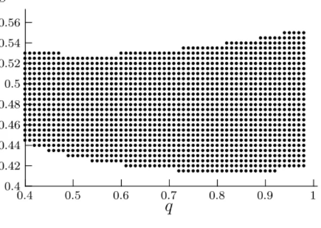
A downward sloping relationship between the probability of getting caught q and criminal activity is easily illustrated in simple examples.

In the following example, v = 0 to focus on stigma costs. A slice of the equilibrium correspondence, plotting the relation between equilibrium s and q.

Every dot indicates an equilibrium switchpoint. This example

0.4 0.42 0.44 0.46 0.48 0.5 0.52 0.54 0.56

0.4 0.5 0.6 0.7 0.8 0.9 1

q s

Figure 1: The Equilibrium Correspondence: s vs. q.

illustrates nicely the possibility of multiple equilibria. The example exhibits the neoclassical relationship between the probability of getting caught and the criminality of the equilibrium strategy over most of its range. But for q large enough, the social interaction effect dominates. The comparative statics changes direction; increasing q increases the criminality of the equilibrium strategy set.

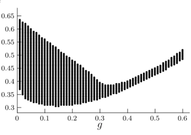
Not surprisingly, similar effects are at work in the relationship be-

tween equilibria and the parameter g, the arrival rate of untaggings. When

Dynamics

12 g increases, the conventional effect is that stigmatic markers are held for a shorter period of time, and so stigma costs decrease. Hence criminal activ- ity should become more likely. The social interaction effect, however, has it that fewer individuals are tagged at any moment in time, and so the flow costs of stigma have increased. The social interaction effect dominates in the downward-sloping part of the following figure.

Expected duration of the

0.3 0.35 0.4 0.45 0.5 0.55 0.6 0.65

0 0.1 0.2 0.3 0.4 0.5 0.6

s

g

Figure 2: The Equilibrium Correspondence: s vs. g.

stigmatic punishment, 1/g, is in fact a policy variable of those courts which administer so-called “shaming-penalties”.

Book (1999) relates that in colo- nial Williamsburg a convicted thief was nailed by his ear to the pillory. At the completion of his sentence his gaolers ripped him from the pillory without first removing the nail, thereby “earmarking” him for life. That is, g = 0.

Overly long punishments can have the perverse effect of reducing the incen- tives to avoid criminal activity. The positive effect on the cost of increasing the waiting time τ is more than offset by the decreases in cost created by changes in the

process.

4 The Equilibrium Tagging Process

The ebb and flow of criminal behavior, long run averages and likely short

run paths, are properties of the population tag process. This process is de-

rived from the equilibrium strategy and the assumptions about the stochastic processes generating crime opportunities, capture, and untagging.

4.1 Birth and Death Rates

Define the population state space S =

1/N, . . . , 1}. Let

denote the population process for a population of size N . This is a birth-death process with birth rates κ

and death rates ν

:

κ

= N (1

n)g ν

= N npσ

N n

1 N

1

q

The argument of σ

is computed as follows. In population state n, an un- tagged individual sees N n

1 other untagged individuals, so the fraction of others who are tagged is m(n) = (N n

1)/N . These birth and death rates completely characterize the population process, including its short run and long run behavior. Let n

and n

denote the next biggest and next smallest states to n, n + (1/N) and n

(1/N ), respectively.

4.2 Equilibrium in the Long Run

For any equilibrium, the long run behavior of the population process is de- scribed by its invariant distribution. The state process is always ergodic.

Since the birth rate is strictly positive for any n > 0, it is possible to reach 1 from any state. Consequently the state process has a unique invariant distri- bution. For instance, if there is a state m

such that no crimes are committed for m > m

, then the unique invariant distribution puts all its mass on the state n = 1.

One virtue of the birth-death formalism is that the invariant distri- bution is easily computed. The invariant distribution π is characterized by the relationship

π(n)κ

= π(n

)ν

Dynamics

14 Iterating this relationship, we have that if there is a state n

such that ν

= 0, then π(n) = 0 for all n < n

, and if n

= max{n : ν

= 0}, then for all n > n

,

π(n) π(n

) =

n⁻

Y

k=n⁰

κ

ν

=

n⁻

Y

k=n⁰

1

k k

g pqσ

N−1

(3) where the index is understood as being incremented in units of size 1/N .

The invariant distribution allows for the calculation of such variables as the long run crime rate. If the population is in state n, the rate at which individuals commit crimes is

η(n) = N (1

n)p + N npσ N n

1 N

1

;

The N (1

n) tagged individuals commit crimes at rate p; every crime that comes their way. The N n untagged individuals commit crimes at the lower rate given by their strategy. The average of this function with respect to the invariant distribution gives the long run crime rate.

The comparative equilibrium analysis of Theorem 2 has straightfor- ward implications for the long run behavior of the population state process.

Let x be a parameter with respect to which equilibrium is increasing. As x increases, the death rates in each state increase. The theorem states that in each state m = (N

N n)/(N

1), the probability of committing a crime is (weakly) increasing, and so, according to the definition, is the death rate ν

. The birth rates are fixed by the parameter g, and so remain unchanged.

Comparative static analysis of equilibrium strategies has straightforward im- plications for changes in death rates, and therefore for changes in the invari- ant distribution.

Theorem 3.

The invariant distribution is non-increasing with respect to parameters F and r in the sense of first-order stochastic dominance, and non-decreasing in c and v.

Corollary 1.

The crime rate η(n) is non-decreasing with F and r, and non-

increasing in c and v.

4.3 Tag Duration in the Long Run

The failure of the conventional intuition to predict the effects of changes in g and q on the criminality of equilibrium strategies depends upon the values of other parameters. Cases other than those presented in the previous section present the predicted comparative statics. But the effects of these parameters is due not just to the equilibrium strategies but also to the rate at which those committing crimes are tagged, and the rate at which they are subsequently untagged. Due to this second effect, the counterintuitive effect of increasing g on the invariant distribution and on the long-run crime rate is universal for large enough parameter values.

Denote by σ

the map from Ω

Not} such that σ(ω, u) = Commit if and only if u

qv

0. Recall that regardless of pa- rameter values, σ

= σ

. Any strategy σ

more criminal than σ

is strongly dominated by it, since the additional opportunities σ

accepts that σ

does not have negative immediate rewards. More generally, if σ

is any reservation strategy which in some recurrent state ω has a threshold u < qv, it is strictly dominated by the strategy which raises the threshold in state ω to qv.

Let η

= p 1

F (qv)

denote the crime rate which would be observed if all untagged individuals acted according to σ

. From these considerations the following lemma is obvious.

Lemma 1.

The long run equilibrium crime rate η(n) is bounded above by η

.

We should expect this upper bound to be achieved for large values of g.

When g is large, the expected duration of a tag is small, and status costs become negligible. The neoclassical effect should dominate the social inter- action effect. This is true, but the bound can also be achieved for small g.

Intuitively, when g is sufficiently small, any tag lasts a very long time. In the long run, most of the population will be tagged most of the time, and therefore most behavior is governed by σ

= σ

, rather than σ

(whatever it may be). Let µ

denote the probability distribution on S which puts all its mass on 0, and let µ

denote point mass at 1.

Theorem 4.

Suppose that F qv + qc(1)/r

< 1. Then lim

µ

= µ

.

Suppose that F (u) is continuous at u = qv. Then lim

µ

= µ

. In both

cases, lim

η(n) = η

.

Dynamics

16 If status costs ever have an impact on choice, then the long run crime rate must be decreasing in g over some range of values.

4.4 The Discrete Example: Short Run, Large N

For any differentiable function f : S

the birth and death rates give a differential equation which characterizes the evolution of the conditional expectation of f through time:

d

dτ E{f (n

)|n

= n}

τ=0

= κ

f(n

)

f(n)

+ ν

f(n

)

f(n)

= κ

f

(n) 1

N

ν

f

(n) 1

N + O(N

)

=

(1

n)g

npσ

m(n) q

f

(n) + O(N

)

If f(n) = n, then d

dτ E{n

= n}

τ=0

= (1

n)g

npσ

m(n)

q + O(N

) The differential equation

˙

n = (1

n)g

npσ

m(n) q

is the mean field equation of the model. For the utility distributions consid- ered in this and the next section, it is of the form

˙

n = (1

n)g

npq(1

) for n < s, (4a)

˙

n = (1

n)g

npq for n > s, (4b) with steady states

n

= g

g + pq(1

) and n

= g g + pq (one for each branch), and solution

n(t) = n

+ n(0)

n

e

for n(0) < s, (5a)

n(t) = n

+ n(0)

n

e

for n(0) > s, (5b) The mean field equation characterizes the behavior of the process over finite time horizons in large populations. The following result is well-known in the literature on density-dependent population processes (Ethier and Kurtz 1986, Chapt. 10, Theorem 2.1).

Theorem 5.

Let

denote a sequence of equilibria in a population of size N , such that the switch points s

converge to a limit s. Suppose that n(t) is the solution to the differential equation (4) from initial condition n

s, and let n

denote the random variable that describes the population state at time t in a population of size N beginning from initial condition n

(0) = n

. Then for all T > 0, lim

sup

n(t)| = 0 a.s.

The steady states are states in which the rate at which untagged individuals are tagged just equals the rate at which tagged individuals are untagged.

The two different steady states correspond to the different rates at which untagged individuals commit crimes above and below the switch point. This is not to say that the two steady states are realized in practice. If for instance, s > n

, then n

is actually in the regime of low criminal activity. Starting from a high state, n

will move downward according to equation (5a) until state s is reached, and then continue moving down through n

according to equation (5b).

4.5 The Discrete Example: Long Run, Large N

In the discrete model with > 0 the equilibrium odds ratios for an equilib- rium with switch point m

and no mixing are given by the following formulas.

Let n

= m

+ (1

m

)/N . π(n)

π(0) =

n⁻

Y

k=0

1

k k

g pqσ

N−1

=











N

N n

g pq(1

)

N n⁻

if n

< n

,

N

N n

g pq(1

)

N nu

g pq

N(n⁻−n^u)

if n

n

.

Dynamics

18 A simple asymptotic approximation describes the shape of the in- variant distribution for large populations. This analysis follows Blume and Durlauf (1998). Let

ρ(n) = 1 n

(1

n)

g pq

min{n,n^u}

g pq(1

)

max{0,n−n^u}

Use Stirling’s formula to estimate the factorials and take limits:

π

(n)

z

ρ(n)

p

2πn(1

n)

where z

is a normalizing factor. Thus the behavior of the invariant distri- bution for large N is governed by the behavior of ρ(n). Taking derivatives of ρ(n) with respect to n, we see that ρ(n) has two local maxima n

and n

, with n

in between. Raising ρ to the power n has the effect of making the function steeper without changing the location of the maxima. Thus the invariant dis- tribution piles up at the steady states of the mean field approximation as N becomes large.

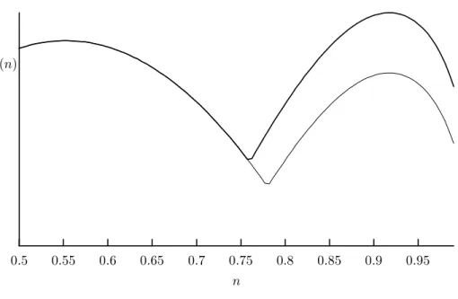
Typically there will be only one global maximum, and so as N becomes large, the invariant distribution will pile up on one and only one of the steady states. That is, the invariant distribution will converge with N to point mass on one of the steady states as N grows large. Which steady state gets the mass in the long run is determined by the location of the limit switch point.

For example, the following plot shows invariant distributions over part of the

range at two different switch points. The parameter values are p = 0.15,

g = 0.1, q = 0.6, r = 0.9, c = 2.5, δ = 1.0 and = 0.1. With these values,

the steady states are n

= 0.552 and n

= 0.917. The range of equilibrium

switch points is (0.752, 0.800). The plot shows the invariant distributions for

switch points n

= 0.76 and n

= 0.78. They share the first piece in common,

because, up to the rescaling coefficient z

, the first piece of the distribution

depends on n

only for its stopping point. When n

= 0.76 the switch comes

earlier, and so the second hump is taller than the first. When n

= 0.78 the

switch is later, and the reverse is true. The invariant distribution tends to

point mass at n

in the latter case, and to point mass at n

in the former

case. Of course it is possible to choose parameter values where there is no

transition. For instance, simply make small.

0.5 0.55 0.6 0.65 0.7 0.75 0.8 0.85 0.9 0.95 ρ(n)

n

Figure 3: Invariant distributions for two different switch points.

5 Conclusion

A complete account of stigma as a social control process requires an analysis of how stigmatic attributions are formed. In fact there are many accounts.

Closest to contemporary decision theory is a model of stereotyping which

recognizes the use of overly simple models for categorization as an efficient

allocation of cognitive resources.

I offer no such account here. Instead I make

micro-level assumptions about the incentive effects of stigma. The driving

assumption of my analysis is that the cost of being stigmatized, however it is

realized, is low when many people bear the marker, and highest when only a

few are so marked. Even this assumption would run afoul of some coherent

theories of stigmatization.

To the extent that stereotyping is a statistical

phenomenon, it is hard to form stereotypes if the incidence of the marker is

low. Here I envision the social control process runing on a time scale which

is short relative to the persistence of stereotypes, so that the stability of the

stigmatic power of particular markers is not at issue. To the extent that the

group at risk of stigmatization is large, the social cost of discipline may be

too high when a large fraction of the group is tagged. The social cost of

Conclusion

20 stigmatizing drunk drivers is small; the wage effects of a social custom not to hire those who park illegally could be enormous. Here I envision that the behaviors being stigmatized are seriously considered by or feasible to a small subset of the total population.

The efficacy of the stigma as a social control mechanism raises the question of if, and how, it can be used as a policy tool. Lessig (1995) offers a lovely anecdote about a government attempt to manipulate the stigma cost function c. In the late 1950’s motorcycle helmets were beginning to leak from western Europe into the Soviet Union, which produced none. For the Soviet leadership, the medical benefits of wearing helmets were exceeded by the so- cial cost of an invasion by a western style. “Thus began an extraordinary and self-conscious campaign by the Soviet government to vilify the wearers of motorcycle helmets. Cartoons appeared in the popular (read: government- controlled) press, mocking the ‘white heads’ on cycles. By the early 1960s, people began wearing helmets only at night, to avoid easy detection.”

Ac- cording to Lessig, helmets were never banned outright, suggesting that the stigmatization of riders was effective enough. Soon enough, however, the So- viets began to produce their own helmets, and with the availability of Soviet helmets, the campaign changed. Instead of stigmatizing helmet-wearers, it switched to stigmatizing those who imported helmets. The stigma cost of wearing helmets fell, and helmet usage increased.

Kahan (1997) claims a more subtle example of stigma manipulation in the policy of rewarding inner-city high school students who turn in peers carrying guns. In his account, not carrying a gun is a stigmatic marker. He argues that the reward policy succeeds because it manipulates stigma as well as having a direct effect on the stock of guns. The stigmatic effect is that when some students are out for the reward, displaying one’s gun becomes more costly. If gun owners become more reluctant to display them, then the meaning of the marker changes, the stigma costs of not carrying falls, and the incentive to carry a gun is reduced.

A third, prominant example of promoting social control through stig-

ma management is the increased use of shaming punishments in the United

States and Great Britain.

In colonial America shaming could be for life. In

modern times, shaming penalties are frequently seen as part of a probation

sentence, a less costly and disruptive approach to behavior modification than

prison for appropriate convicts.

As a tool of social control, stigma can be mismanaged. Theorem 4 shows that increasing the duration of stigma (decreasing g ) will ultimately increase the long run crime rate. The largest possible crime rates are achieved when the duration is extremely long. This point is not merely of academic interest. Third strike drug offenders are banned for life from receiving a variety of federal benefits, including food stamps and temporary assistance to needy families available under the Personal Responsibility and Work Op- portunity Reconciliation Act of 1996.

In some states, businesses requiring licenses cannot obtain them if they employ convicted felons, no matter how old the offense. This effective lifetime employment ban bars former convicts from working in, among other locations, barber shops and automobile body shops. In a similar vein, easy access to criminal records makes it easier for employers not obligated by law to nonetheless turn down applicants with criminal records. For instance, The Fair Credit Reporting Act prohibited the reporting of convictions more than seven years old, until this provision was deleted in 1998.

This information be be socially useful for its signal value, but Theorem 4 suggests that the availability of such old information may well have a negative deterrent effect on crime.

Another important counter-productive effect of stigmatization is not captured in this model. When “normal” society shuns the stigmatized, some may seek to shed the stigma (for instance, by having physical deformities corrected) or to overcome it by excelling in other dimensions. Others may respond by joining together with other stigmatized individuals to create

“counter-communities” — communities in which the stigmatized activity is ignored or even becomes a source of status.

Newman (1999) writes about the stigma teenagers attached to “flipping burgers” in Harlem and other poor New York neighborhoods and, in particular, about the strategies young workers employ to defend themselves against the jokes and ridicule directed at them.

. . . it is clear that the workplace itself is a major force in the

creation of a ‘rebuttal culture’ among these workers. Without

this haven of the fellow-stigmatized, it would be very hard for

urger barn employees to retain their dignity. With this support,

however, they are able to hold their heads up, not by definining

Conclusion

22 themselves as separate from society, but by callking upon their commonality with the rest of the working world.

Informal social control of deviance presumes a community which is sufficiently cohesive, well-organized, and has sufficient resources to enforce social norms. Elijah Anderson’s (1990) ethnography of “Northton” describes the how the clash between “decent” norms (family life, hard work, church- going) and “streetwise” norms (associated with crime and the drug culture) is facilitated by a weakened structural fabric. The negative correlation of social organization and crime rates appears in empirical analyses as well.

Sampson and Groves (1989) found in British data that neighborhoods with lower levels of social organization had higher levels of violent and property crimes. Unsupervised teen groups were the largest contributors to the violent crime rate, while local friendship networks and organizational participation had a large negative impact on robbery. Most surprisingly, the effect of the measured indices of social organization on crime exceeded the direct effects of socio-economic status. One source of disrupted friendship networks and broken families is the high incarceration of young male African-Americans.

The legislative response to the crack epidemic of the 80’s has been massive mandatory minumum sentences.

A reinforcing effect of stigma not captured here is its effect on labelling the boundaries of normative behavior. When Hester Prynne is marked with the scarlet letter ‘A’, not only is she stigmatized, but the community reaffirms for itself the labelling of adulterous behavior as deviant. A contemporary (and perhaps non-fictional) instance of this labelling effect is the so-called

“broken windows” theory which lies behind “order maintenance policing”.

Lessig (1995), Kahan (1997) and others argue that the power of law to es- tablish social boundaries and create categories for stigmatization is not yet fully appreciated as a source of social control.

The account of stigma and the enforcement of social norms presented

here extends the evolutionary game theory paradigm by offering a richer

account of individual choice. In particular, forward looking behavior is rarely

studied, and almost never in stochastic models.

Stigma is in essence a

dynamic phenomena. Its costs are born in the future, and the magnitude

of those costs are determined by the future actions of others. This is why

the pop rational actor social science accounts which, at their best, make

reference to some kind of evolutionary game dynamics in a coordination game, seem so shallow. For instance, it would be hard to formulate a question about the effect of punishment duration in such models. The subject of evolutionary game theory is the dynamics of player choice. Recognizing players as intertemporal decision makers models opens up a variety of new modelling opportunities. Evolutionary game theory has been nearly devoid of serious applications to the social sciences. The premise of this paper is that deeper models of individual choice will provide evolutionary game theory with the wherewithal to address social issues.

6 Proofs

This section contains proofs of Theorems 1 through 4 and details on com- puting equilibria.

6.1 Theorems 1, 2 and 3

The proofs of Theorems 1 and 2 rely on the strategic complementarity that works through the stigma cost of crime. More criminal strategies lead to more tagged individuals, which lowers the stigma costs, thereby making crime more profitable. The complementarity appears twice in the proof: First to show that the optimal response to any strategy is a monotonic reservation strategy, and second to work the fixed point argument to get the existence of equilibrium results and to sign the dependence of the equilibrium strategy set on parameters.

In the individual’s decision problem, states are the number of others who are tagged. The assumptions of the model implies that each individual takes the state process to be a birth-death process with some given rates.

States evolve, and independently, events happen. An event is the arrival

of either a criminal opportunity or an untagging. The event process is the

superposition of two independent Poisson processes: A rate p process for

criminal opportunities and a rate g process for untaggings. The event process

is a rate p + g Poisson process, and the probability that a given event is a

Proofs

24 criminal opportunity is p/(p+g). Types of events are uncorrelated over time.

See Kingman (1993) for details.

Construction of value functions and evaluation of policies involves comparing the values of functionals along paths of the state process. This is done with a coupling argument. Let ω denote a path of the birth-death process

, and define the function f (ω) =

0

e

g(ω

)dt on paths.

Lemma 2.

If

is a birth-death process and g(m) is non-decreasing in m, Then E{f(ω)|ω

= m} is non-increasing in m. If g(m) is not constant, then the conditional expectation is strictly decreasing in m.

Proof

. Choose m

< m

, and construct the stochastic process

, y

)}

with (x

, y

) = (m

, m

) as follows: Let s = inf{t : x

y

denote the coupling time of the x

and y

processes. Let x

evolve according to the birth and death rates of the m

-process. Let y

evolve according to the rates for the m

-birth-death process, independently so long as x

< y

, that is, so long as t < s. Observe to that almost surely s <

and that x

= y

. Let y

= x

for t

s. Observe that each marginal process is a birth-death process evolving according to the rates for the m

-process. Furthermore, almost surely x

y

for all t.

Now consider the flows g(x

) and g(y

). Clearly g(x

)

g(y

) almost surely for all t. Consequently for almost all (x

, y

) paths,

Z ∞ 0

e

g(x

)dt

0

e

g(y

)dt

The expectation of the left hand side is E{f (ω)|ω

= m

and the expectation of the right hand side is E{f(ω)|ω

= m

are decreasing in m. If g(m) is not constant, there is a state m

such that c(m) < c(n) for all m

m

< n. For any (x

, y

) path such that for some interval of time, x

m

< y

, the inequality is strict. The set of such paths has positive probability, and so the inequality between conditional expectations is strict.

The first application of this Lemma 2 compares the present discounted

value of the flow cost of being tagged from one criminal opportunity to the

next. An event is the arrival of either the next criminal opportunity or thenext untagging. The time to the next event, τ, is distributed exponentially with parameter p + g . Define

C(m) = E

Z τ 0

e

c(m

)dt

m

= m

= E

Z ∞ 0

e

c(m

)dt

m

= m

To save space below, any expectation operator containing m in the subscript will denote an expectation conditional on the event

= m}. Everything to the right of the vertical line will be surpressed.

Lemma 3.

C(m) is non-decreasing in m, and strictly increasing in m if c(m) is not constant.

Proof.

Integrating by parts, C(m) =

0

e

c(m

)dt. The conclusion follows from Lemma 2.

The next application compares the present discounted value of non-flow costs realized at events.

Lemma 4.

If

is a birth-death process, f(m) is a non-increasing function of m for each t and τ is the arrival time of the next event, then the conditional expectation E

f (m

)} is non-increasing in m.

Proof.

This is another application of Lemma 2.

E

f(m

)} = (p + g)

0

e

f(m

)dt and the conclusion follows from the Lemma.

Suppose an individual has a decision opportunity at time 0. Let τ

denote the time to the next event and σ denote the time to the next crim-

inal opportunity after τ . Then τ and σ are distributed independently and

Proofs

26 exponentially, τ with parageter p + g and σ with parameter p. Let V (m, δ) denote the value of optimal choice for an untagged individual in state m with net expected reward δ, and let W (m, δ) denote the same reward for a tagged individual. For any function f (m, δ), let ˆ f(m) = E

f(m, δ), the result of expecting out u (which is independent of all other random variables in the model). Define V

(m, δ) to be the value to an untagged individual of mak- ing decision x

(Commit or Not) and continuing optimally. Define W

(m, δ) similarly for tagged individuals.

Begin with tagged individuals:

W

(m, δ) = δ

C(m) + E

n

e

g

p + g E

e

V ˆ (m

) + p

p + g W(m ˆ

)

W

(m, δ) = 0

C(m) +

If the individual commits the crime, she receives expected immediate net reward δ. She also pays a flow cost of being tagged until the next event. The expected value of this cost is C(m). With probability g/(p + g) that event is an untagging. She then waits, without paying tagging costs, until the next crime opportunity, at which time she plays optimally. With probability g/(p + g ) that event is a criminal opportunity, and she plays optimally, still tagged. This gives W

(m, δ). A similar explanation covers W

(m, δ).

The one-step deviation principle implies that the optimal strategy for a tagged player has

σ

(m, δ)







{C}

if δ > 0,

if δ = 0,

if δ < 0.

Furthermore

W (m, δ) = max{W

(m, δ), W

(m, δ)}

= max{δ, 0} − C(m) + E

n

e

g

p + g E

e

V ˆ (m

) + p

p + g W ˆ (m

)