IHS Economics Series Working Paper 294
December 2012
Spatial System Estimators for Panel Models: A Sensitivity and Simulation Study
Shuangzhe Liu
Impressum Author(s):
Shuangzhe Liu, Tiefeng Ma, Wolfgang Polasek Title:
Spatial System Estimators for Panel Models: A Sensitivity and Simulation Study ISSN: Unspecified
2012 Institut für Höhere Studien - Institute for Advanced Studies (IHS) Josefstädter Straße 39, A-1080 Wien
E-Mail: o ce@ihs.ac.atffi Web: ww w .ihs.ac. a t
All IHS Working Papers are available online: http://irihs. ihs. ac.at/view/ihs_series/
This paper is available for download without charge at:
https://irihs.ihs.ac.at/id/eprint/2177/
Spatial System Estimators for Panel Models: A Sensitivity and Simulation Study
Shuangzhe Liu, Tiefeng Ma, Wolfgang Polasek
294
Reihe Ökonomie
Economics Series
294 Reihe Ökonomie Economics Series
Spatial System Estimators for Panel Models: A Sensitivity and Simulation Study
Shuangzhe Liu, Tiefeng Ma, Wolfgang Polasek
December 2012
Contact:
Shuangzhe Liu University of Canberra Canberra, Australia
email: shuangzhe.liu@canberra.edu.au Tiefeng Ma
Statistics College
Southwestern University of Finance and Economics Chengdu 610074, China
email: cdtf.ma@gmail.com Wolfgang Polasek
Department of Economics and Finance Institute for Advanced Studies Stumpergasse 56
1060 Vienna, Austria
: +43/1/599 91-155 email: polasek@ihs.ac.at
Founded in 1963 by two prominent Austrians living in exile – the sociologist Paul F. Lazarsfeld and the economist Oskar Morgenstern – with the financial support from the Ford Foundation, the Austrian Federal Ministry of Education and the City of Vienna, the Institute for Advanced Studies (IHS) is the first institution for postgraduate education and research in economics and the social sciences in Austria. The Economics Series presents research done at the Department of Economics and Finance and aims to share “work in progress” in a timely way before formal publication. As usual, authors bear full responsibility for the content of their contributions.
Das Institut für Höhere Studien (IHS) wurde im Jahr 1963 von zwei prominenten Exilösterreichern – dem Soziologen Paul F. Lazarsfeld und dem Ökonomen Oskar Morgenstern – mit Hilfe der Ford- Stiftung, des Österreichischen Bundesministeriums für Unterricht und der Stadt Wien gegründet und ist somit die erste nachuniversitäre Lehr- und Forschungsstätte für die Sozial- und Wirtschafts- wissenschaften in Österreich. Die Reihe Ökonomie bietet Einblick in die Forschungsarbeit der Abteilung für Ökonomie und Finanzwirtschaft und verfolgt das Ziel, abteilungsinterne Diskussionsbeiträge einer breiteren fachinternen Öffentlichkeit zugänglich zu machen. Die inhaltliche Verantwortung für die veröffentlichten Beiträge liegt bei den Autoren und Autorinnen.
Abstract
System of panel models are popular models in applied sciences and the question of spatial errors has created the recent demand for spatial system estimation of panel models.
Therefore we propose new diagnostic methods to explore if the spatial component will change significantly the outcome of non-spatial estimates of seemingly unrelated regression (SUR) systems. We apply a local sensitivity approach to study the behavior of generalized least squares (GLS) estimators in two spatial autoregression SUR system models: a SAR model with SUR errors (SAR-SUR) and a SUR model with spatial errors (SUR-SEM). Using matrix derivative calculus we establish a sensitivity matrix for spatial panel models and we show how a first order Taylor approximation of the GLS estimators can be used to approximate the GLS estimators in spatial SUR models. In a simulation study we demonstrate the good quality of our approximation results.
Keywords
Seemingly unrelated regression models, panel systems with spatial errors, SAR and SEM models, generalized least-squares estimators, Taylor approximations
JEL Classification
Contents
1 Introduction 1
2 SAR-SUR models and their estimators 3
2.1 Simple GLS estimators of the SAR-SUR model ... 3 2.2 The reduced form of the SAR-SUR model ... 5 2.3 Special case: common spatial SAR correlation coefficient ... 7
3 Approximating the GLS estimator in the SUR-SEM model 9
3.1 SUR models with SEM errors ... 9 3.2 Special case: a common θ correlation coefficient in the SUR-SEM model ... 12
4 Simulation study: how good are Taylor approximations of
GLS estimates? 14
5 Conclusions 19
References 20
6 Appendix 21
6.1 A1: Some mathematical definitions and properties ... 21 6.2 A2: Alternative evaluation of the simulation study by distances ... 22
1 Introduction
Spatial models and applications in statistics and econometrics have been stud- ied in the past decades; see e.g. Paelinck and Klaassen (1979), Anselin (1988, 2010), Florax and Van Der Vlist (2003), Haining (2003), LeSage and Polasek (2008), LeSage and Pace (2009), and Liu et al. (2012). On the other hand, panel models have become increasingly important and different estimators in such models with spatial components have also been studied; see e.g. Kapoor et al. (2007), Anselin et al. (2008), Baltagi (2008), Elhorst (2010), and Lee and Yu (2010). It is clearly useful to examine the sensitivity of these estimators in terms of a minor change in the spatial correlation parameter ρ.
The usual spatial auto-regression (SAR) model for the n
×1 cross-sectional observations y is given by
y = ρW
ny + Xβ + u, u
∼N[0, σ
2I
n]. (1) In a similar way we define the SEM model:
y = Xβ + e, with e = θW
ne + u, (2)
where we assume a heteroskedastic error term for u :
E(u) = σ
2D
v, t, s = 1, ..., T.
Sensitivity analysis with respect to ρ means we are interested in the behavior of the estimators of β upon a small change of ρ. The numerical computation of the ”spatial filter” estimator of spatial autoregression (SAR) models uses the spatial filter matrix R = I
−ρW , which acts as a filter in the reduced form of the SAR model. Spatial estimators are a function of the spatial neighborhood matrix W , which can become really large in large spatial panel systems, and the spatial correlation parameter ρ.
Our question is if ’good’ approximations of simple spatial estimators exist to justify a reasonable sensitivity analysis (or making a spatial diagnostics without employing a time consuming spatial estimation procedure), and if so, what estimators and what GLS estimation approaches should be considered to use for diagnostics or approximations? A previous study of the sensitivity of spatial estimators, like the cross-sectional SAR and the SEM model, has been made in Liu et al. (2012). It was shown that good approximations exists for small values of the spatial correlation parameter.
The present paper extends a system of panel models to a seemingly unrelated
regression (SUR) system with spatial errors in two ways: one is a SAR regres-
sion model with SUR errors (SAR-SUR) and the other is a SUR model with spatial errors model (SUR-SEM). First, we propose a system least squares (SUR based) estimator with spatially filtered variables, which is the SF-GLS estimator and we show that it can be expanded in a first order Taylor series around the non-spatial GLS estimator of a non-spatial regression model. The second type of system (or SUR based) estimator is the reduced form (RF) estimator, which is a GLS estimator that amounts to spatially transform all dependent and independent variables and is called RF-GLS estimator.
While in a cross-sectional SAR or SEM model we have to explore the sensitiv- ity with respect to only one spatial parameter, we need in the system case a vector of spatial parameters, i.e. for each cross-sectional sample an own spatial correlation parameter. To get the sensitivity result using matrix derivatives for a vector of correlation parameters, we use a simple trick that is found in Magnus and Neudecker (1999). Because we are only interested in the deriva- tive with respect to the diagonal matrix, we first derive the matrix-to-matrix derivative and then in a last step we employ the general result, that a di- agonal derivative can be obtained by post-multiplying the matrix-to-matrix derivative with the selection matrix J, presented in Appendix.
Thus, we are also interested if simplifications of the system sensitivity results are possible if we make the simplifying assumptions, that there exists only one common spatial correlation parameter, briefly called the ”cc-case”. Luckily, in the SAR-SUR system case we gain no new insights by doing these simplifi- cations, we find for the SAR-SEM model nice interpretations in the line of global sensitivity analysis as in Leamer (1978). The spatial correlation param- eter traces out a hyper-curve between two simpler non-spatial estimators.
For the simulation study we develop a basic design involving the number of observations, the neighborhood matrix W and the SUR covariance matrix Σ to compute the average MSE or MPLS for the evaluation of the estimators.
We also discuss how to measure the distance between the GLS estimator and its first order Taylor approximation in dependence of the spatial parameter ρ.
The structure of paper is as follows. In section 2, we consider the SAR-SUR model and their estimators. We derive the sensitivity results with respect to the two types of spatial correlation parameters (SAR or SEM). In section 3, we study the SUR-SEM model and the Taylor approximation sensitivity re- sults. A simulation study for different sample sizes to check the quality of the approximate GLS estimates together with a comparison of the two estimators, the spatial filter estimator and the reduced form estimator are presented in section 4. Our concluding remarks are made in section 5. Finally, some basic definitions and their relevant mathematical properties are presented in the appendix, together with our detailed evaluation of the simulation study.
2
2 SAR-SUR models and their estimators
In this section, we consider the SAR model (1) and the extension of the model to a panel system. This leads to a system of regression equations and a seem- ingly unrelated regression (SUR) specification of the residual variance matrix, as in e.g. Anselin et al. (2008).
2.1 Simple GLS estimators of the SAR-SUR model
First we discuss the system or panel SAR model with a SUR error structure and the simple GLS estimators for this model. The following spatial auto- regression (SAR) model is as in Anselin et al. (2008, pp 637-638) for time t = 1, ..., T
y
t= ρ
tW
Ny
t+ X
tβ
t+ e
t, with E(e
te
′s) = σ
tsI
N, f or t
6=s, (3) where ρ
tis the spatial AR (SAR) correlation parameter for time t, y
tis the N
×1 dependent variable, W
Nis the N
×N neighborhood matrix, X
tis the N
×k regressor matrix, β
tis the k
×1 regression coefficient, e
tis the N
×1 error term, σ
tsis the temporal covariance parameter between time s and t (for convenience, the variance terms are expressed as σ
t2), and I
Nis the N
×N identity matrix.
In compact form, the SAR-SUR model for T cross-sections is given by
y = (D
ρ⊗W
N)y + Xβ + e, with e
∼N [0
N T, Σ
sur] (4) where y = (y
1′, ..., y
′T)
′= vecY is a NT
×1 vector obtained from Y which is a N
×T dependent panel matrix, vec is the vectorisation operator (see e.g. Neudecker et al. 1995a, 1995b), D
ρ= diag(ρ
1, ..., ρ
T) is a T
×T diagonal matrix, X = diag(X
1, ..., X
T) is an NT
×kTmatrix with X
tof order N
×k,β = (β
1′, ..., β
T′)
′contains the kT
×1 system regression coefficients, e = (e
′1, ..., e
′T)
′is the error vector and its covariance matrix is
Σ
sur=
E(ee
′) = Σ
T ⊗I
N(5) with a T
×T positive definite covariance matrix Σ
Tfor the SUR system.
Assuming normal errors, the log-likelihood function (ignoring the constants)
is given by
L = ln
|IN T −D
ρ⊗W
N|+ 1
2 ln
|Σ−sur1| −1
2 e
′(Σ
−sur1)e
= Σ
Tt=1ln
|IN −ρ
tW
N|+ N
2 ln
|Σ−T1| −1
2 e
′(Σ
−T1⊗I
N)e,
where the error term is e = (I
N T −D
ρ⊗W
N)y
−Xβ. For further details see Anselin (1988, pp 145-146) and Anselin et al. (2008 p. 650).
Definition
1: The spatial filter SF-GLS estimator ˆ β
G.
We consider the spatial filter (SF) form of the SAR-SUR panel model (4)
R
N Ty = Xβ + e with e
∼N [0, Σ
sur]. (6) The generalized LS (GLS) estimator is then given by
β ˆ
G= (X
′Σ
−sur1X)
−1X
′Σ
−sur1R
N Ty, (7) where
E(ee
′) = Σ
sur= Σ
T ⊗I
Nis the SUR covariance matrix (5), and the system spread matrix is R
N T= I
N T −D
ρ⊗W
N.
Denote the T
×1 vector of spatial correlations p = (ρ
1, ..., ρ
T)
′of the SAR- SUR system in (4). When p = 0 we get D
ρ= 0 and the simplification of the filter matrix R
N T= I
N Tto the homoskedastic case, such that the spatial GLS estimator reduces to the non-spatial (panel) GLS estimator, which is the SUR estimator for equation systems
β ˆ
gls= (X
′(Σ
−T1⊗I
N)X)
−1X
′(Σ
−T1⊗I
N)y. (8)
Next, we derive the sensitivity of the GLS estimator and the Taylor approxi- mation of ˆ β
Gwith respect to p, using Magnus and Neudecker’s (1999) matrix differential calculus; for their differential idea, see part A1 in Appendix 6.
Theorem 1
The kT
×T sensitivity matrix of the GLS estimator (7) of the spatial SAR-SUR panel model (4) with respect to p = (ρ
1, ...ρ
T)
′is
S
G= ∂ β ˆ
G/∂p
′=
−(X′Σ
−sur1X)
−1X
′Σ
−sur1(I
T ⊗W
NY ) J (9) where J is the T
2 ×T selection matrix given in (10) and Y = (y
1, ..., y
T) is the N
×T de-vectorized (or stacked) panel matrix such that vec Y = y.
4
Proof: In the SAR-SUR system the spread matrix is
R
N T= I
N T −D
ρ⊗W
Nand we find the derivative with respective to p d R
N Ty =
−d(Dρ⊗W
N)vec Y
=
−vec(W
NY dD
ρ)
=
−(IT ⊗W
NY )vec (dD
ρ)
=
−(IT ⊗W
NY )J dp,
where vec is the vectorisation operator, J is the T
2×T selection matrix for diagonal derivatives, defined as
J = (i
1⊗i
1, ..., i
T ⊗i
T) (10) with I
T= (i
1, ..., i
T) being a T
×T identity matrix, and
⊗denotes the matrix Kronecker product; for these definitions and the relevant properties, see part A1 of the Appendix 6.
Therefore, for the differential of the SAR-SUR GLS estimator (7) of the spatial filter form we find
d β ˆ
G= d [(X
′Σ
−sur1X)
−1X
′Σ
−sur1R
N Ty]
=
−(X′Σ
−sur1X)
−1X
′Σ
−sur1(I
T ⊗W
NY )J dp. (11) This establishes the theorem.
Note that S
Gis free of the correlations in p and hence we obtain a simple expression of the derivative matrix S
G0= S
G|p=0= S
G.
Theorem 2
The first order Taylor approximation of the SF-GLS estimator β ˆ
Gin (7) of the SAR-SUR panel model is
β ˆ
G≈β ˆ
gls+ S
G0p, (12)
where β ˆ
Gis the kT
×1 vector and S
G0is the kT
×T sensitivity matrix in (9).
Proof: Use the Taylor series expansion.
2.2 The reduced form of the SAR-SUR model
From the SF form of the SAR-SUR panel model
R
N Ty = Xβ + e with e
∼N [0, Σ
sur] (13) with
E(ee
′) = Σ
sur= Σ
T ⊗I
N, we get the reduced form of the SAR-SUR model with R
N T= I
N T −D
ρ⊗W
Nto be
y = R
−N T1Xβ + R
−N T1e with R
−N T1e
∼N [0, Σ
eN T] (14) and
Σ
eN T= var(R
−N T1e) = R
−N T1Σ
surR
′−N T1= (R
′N TΣ
−sur1R
N T)
−1. (15) Note that the GLS estimator in the reduced form of the SAR-SUR model is the same as ˆ β
Gin (7). Next we consider a GLS estimator.
Definition
2: The GLS estimator in the reduced form SAR-SUR model ˆ β
z. The reduced form GLS estimator of the SAR-SUR model (14) is just the OLS estimator in terms of the transformed regressor
β ˆ
z= (Z
′Z)
−1Z
′y with Z = R
−N T1X or
β ˆ
z= Z
+y with Z
+= (X
′R
N T−1 ′R
−N T1X)
−1X
′R
−N T1′. (16) For the special case with p = 0 we get R
N T= I
N Tand then the GLS estimator simply becomes the OLS estimator of the untransformed panel system
β ˆ
ols= (X
′X)
−1X
′y.
Theorem 3
In the SAR-SUR model in (14), the sensitivity of the reduced form GLS estimator (16) is the kT
×T matrix
S
z= ∂ β ˆ
z/∂p
′= Z
+(I
T ⊗W
N′E
1)J
−Z
+R
−N T1(I
T ⊗W
NY ˆ
gls)J
= Z
+Q J (17)
with
Q = (I
T ⊗W
N′E
1)
−R
−N T1(I
T ⊗W
NY ˆ
gls)
where Z = R
−N T1X is the transformed regressor, E
1is de-vectorized residual matrix obtained from vecE
1= R
N T′−1(I
−ZZ
+)y = R
′−N T1(y
−y ˆ
gls), and the GLS fit Y ˆ
glsis computed from vec Y ˆ
gls= ˆ y
gls= ZZ
+y.
Proof: Because the differential of the inverse matrix of
R
N T= I
N T−Dρ⊗W
Nwith respect to p is d R
−N T1=
−R−N T1(d R
N T)R
−N T1, dR
N T=
−(dDρ)
⊗W
Nand vec dD
ρ= Jdp, we get for (16)
6
d β ˆ
z= d((Z
′Z )
−1Z
′y)
=
−(Z′Z)
−1(d(Z
′Z ))(Z
′Z)
−1Z
′y + (Z
′Z)
−1(dZ
′)y
= Z
+(dD
ρ⊗W
N′)R
N T′−1(I
−ZZ
+)y
−Z
+R
−N T1(dD
ρ⊗W
N)ZZ
+y
= Z
+(dD
ρ⊗W
N′)vecE
1−Z
+R
−N T1(dD
ρ⊗W
N)vec Y ˆ
gls= Z
+vec(W
N′E
1dD
ρ)
−Z
+R
−N T1vec(W
NY ˆ
glsdD
ρ)
= Z
+(I
T ⊗W
N′E
1)vec(dD
ρ)
−Z
+R
N T−1(I
T ⊗W
NY ˆ
gls)vec(dD
ρ)
= Z
+(I
T ⊗W
N′E
1)J dp
−Z
+R
−N T1(I
T ⊗W
NY ˆ
gls)J dp.
We establish the theorem by rearranging terms.
Theorem 4
The first order Taylor approximation of the RF-GLS estimator of the SAR-SUR model in (16) is
β ˆ
z ≈β ˆ
ols+ S
z0p, (18) where
S
z0= (X
′X)
−1X
′[I
T ⊗E ˜
0]J (19) is the first order sensitivity matrix S
zevaluated at the origin p = (ρ
1, ..., ρ
T)
′= 0, E ˜
0= W
N′Y
−(W
N′+ W
N) ˆ Y
0, Y ˆ
0is de-vectorized from the OLS fit vec Y ˆ
0= X(X
′X)
−1X
′y, and vec Y = y is the vectorized panel matrix.
Proof: From Theorem 3 we get
S
z0= ∂ β ˆ
z/∂p
′|p=0= (X
′X)
−1X
′[I
T ⊗W
N′Y ]J
−(X
′X)
−1X
′[I
T ⊗W
N′Y ˆ
0]J
−(X′
X)
−1X
′[I
T ⊗W
NY ˆ
0]J (20) and then the Taylor approximation follows.
2.3 Special case: common spatial SAR correlation coefficient
We get a special case of the SAR-SUR model (4) when all the spatial corre- lations across the system are equal ρ
1= ... = ρ
T= ρ. In this case we have D
ρ= ρI
Twith ρ being the common correlation coefficient and the model re- duces to the simple SAR regression model as in Anselin et al. (2008)
y = ρ(I
T ⊗W
N)y + Xβ + u (21)
where the error term u = (u
′1, ..., u
′T)
′is a N
×1 error vector and follows a
normal distribution with a NT
×1 mean vector centered at 0 and a NT
×NT
variance matrix σ
2I
N T. Also y = vecY is an NT
×1 vectorized panel vector, ρ is the common spatial autocorrelation parameter (a scalar), W
N T= I
T ⊗W
Nis a system common neighborhood matrix W
Nis the N
×N spatial weight matrix normalized with row sums 1, X is an NT
×kT regressor matrix, and β is a kT
×1 regression coefficient vector.
The panel spatial filter (SF-GLS) estimator b
ρ: kT
×1 of the SAR-SUR model(4) can be written in analogy to the non-system case as a linear combination of 2 simpler GLS estimators
b
ρ= (X
′Σ
−sur1X)
−1X
′Σ
−sur1R
N Ty
= (X
′Σ
−sur1X)
−1X
′Σ
−sur1(I
N T −ρW
N T)y
= (X
′Σ
−sur1X)
−1X
′Σ
−sur1y
−ρ(X
′Σ
−sur1X)
−1X
′Σ
−sur1W
N Ty
= b
0−ρ(X
′Σ
−sur1X)
−1X
′Σ
−sur1W
N Ty
= b
0−ρb
1. (22)
We see that the difference between the SUR-GLS estimator β ˆ
sur= (X
′Σ
−sur1X)
−1X
′Σ
−sur1y
and the spatial lag estimator ˆ β
sur −b
ρ= ρ β ˆ
lagis proportional in size to the spatial parameter ρ and the first order spatial lag estimator
β ˆ
lag= (X
′Σ
−sur1X)
−1X
′Σ
−sur1W
N Ty. (23)
Next we compute the derivative of b
ρwith respect to the common ρ, which measures the sensitivity of b
ρwith respect to a small change in ρ. For analytical and mathematical convenience, we use the differential notation from where the derivative can be obtained equivalently and more easily; see Magnus and Neudecker (1999) and Liu and Neudecker (2009).
Theorem 5
The sensitivity or first derivative of the spatial filter b
ρestimator in the common correlation model with respect to the ρ parameter is the negative spatial lag estimator in the linear model for explaining the first order spatial lag
∂b
ρ/∂ρ =
−(X′Σ
−sur1X)
−1X
′Σ
−sur1W
N Ty =
−β ˆ
lag, (24) where the spatial lag estimator β ˆ
lagis given in (23).
Proof
The matrix differential of the b
ρestimator with respect to ρ in (22) is
db
ρ=
−β ˆ
lagdρ
and by rearranging terms, we establish the derivative.
8
2.4 The common correlation (cc) SAR model
In some cases it might be interesting to look at SAR models that have a common correlation and common coefficient. For practical applications like model choice this can be a good starting point.
The stacked panel SUR-SAR model has the same structure as the model (4) before
y = (D
ρ⊗W
N)y + Xβ + e, with e
∼N [0
N T, Σ
sur] (25) where y = (y
1′, ..., y
T′)
′= vecY is a NT
×1 vector, Y is an N
×T dependent panel matrix, the diagonal matrix D
ρ: T
×T reduces in the cc case to ρI
T, X = (X
1′, ..., X
T′)
′is an NT
×k stacked regressor matrix with X
tof order N
×k, β = (β
1, ..., β
k)
′is a k
×1 vector of stacked regression coefficients.
Assuming a common correlation and common coefficient (cc&cc), we simplify the model structure of the GLS estimator, because R
N T= I
T ⊗R
Nwith R
N= I
N −ρW
N, Σ
sur= Σ
T ⊗I
N, and then the covariance matrix (15) reduces to
Σ
c= (Σ
−T1⊗R
′NR
N)
−1(26) Therefore the GLS estimator in the cc case takes the form
β ˆ
c= (X
′Σ
−c1X)
−1X
′Σ
−c1y, (27) which is the SUR estimator with common spatial heteroskedasdicity of the form R
′NR
N, because Σ
−sur1is the covariance/correlation matrix across the equations of the panel system. This estimator is a SUR-GLS estimator for the spatial transformed (SEM filtered) variables X
∗= (I
T ⊗R
N)X and y
∗= (I
T ⊗R
N)y: ˆ β
c= (X
∗′Σ
−sur1X
∗)
−1X
∗′Σ
−sur1y
∗.
3 Approximating the GLS estimator in the SUR-SEM model
This section computes the sensitivity of the GLS estimator in the SUR-SEM model and describes the first order Taylor approximation using the sensitivity results.
3.1 SUR models with SEM errors
In this section we look at a system generalization of the spatial error model
(SEM), which can be found as alternative to the SAR-SUR model in e.g.
LeSage and Pace (2009).
Consider the following panel SUR-SEM model
y
t= X
tβ + e
t, with e
t= θ
tW
Ne
t+ u
t, (28) where we assume a centered homoskedastic error term for u :
E(u
t, u
′s) = σ
tsI
N(t, s = 1, ..., T ). Now the error term in the SUR-SEM model can be written as
e
t= (I
N −θ
tW
N)
−1u
t= B
N,t−1u
t, (29) where B
N,t= I
N−θ
tW
Nis the t-th component of the SEM filter matrix B
N T. In the cc case the cross-equation covariance matrix between the error vectors e
tand e
sthen becomes
E
[e
te
′s] = B
N−1E[u
tu
′s]B
N−1′= σ
tsB
N−1B
N−1′= σ
ts(B
N′B
N)
−1. (30)
Definition
3: The spatial SUR-SEM model.
In matrix form, the SUR-SEM model with the NT
×1 error vector e can be written as
y = Xβ + e, with e = B
N T−1u, or
y
∼N [Xβ, Σ
sem] with Σ
sem= B
N T−1(Σ
T ⊗I
N)B
N T′−1(31) where the error term u contains the SUR correlation matrix
E(uu
′) = Σ
T⊗IN, and the SUR-SEM system filter matrix
B
N T= I
N T −D
θ⊗W
Nwith D
θ= diag(θ
1, ..., θ
T) (32) is a T
×T diagonal SUR-SEM correlation parameter matrix. Furthermore, y = (y
′1, ..., y
T′)
′= vecY : NT
×1 is the vectorized panel matrix, X = diag(X
1, ..., X
T) is a NT
×KT block-diagonal regressor matrix, and e = (e
′1, ..., e
′T)
′is the error vector.
Note that the log-likelihood function of the SUR-SEM model (31) is
L = 1
2 ln
|BN T′(Σ
−T1⊗I
N)B
N T| −1
2 e
′B
N T′(Σ
−T1⊗I
N)B
N Te
= 1
2 ln
|Σ−sem1 | −1
2 e
′Σ
−sem1e (33)
10
Definition
4: The spatial SEM-GLS estimator ˆ β
sem.
The SEM-GLS estimator in the SUR-SEM model (31) is the kT
×1 vector
β ˆ
sem= [X
′Σ
−sem1X]
−1X
′Σ
−sem1y. (34)
Define the SEM correlation parameter vector as q = (θ
1, ..., θ
T)
′. For zero correlation q = 0, the SEM filter vanishes to B
N T= I
N T, and the GLS estimator in the SUR-SEM model reduces to the GLS type SUR estimator (8).
Theorem 6 (The sensitivity of
β ˆ
sem)Let q = (θ
1, ..., θ
T)
′be the correla- tion vector, then will use the classical sensitivity results. The kT
×T sensi- tivity matrix of the reduced form RF-GLS estimator in the SUR-SEM model is
S
sem= ∂ β ˆ
sem/∂q
′=
−[X′Σ
−sem1X]
−1X
′(I
T ⊗W
N′M Σ
−T1) J
−[X′
Σ
−sem1X]
−1X
′B
N T′(Σ
−T1⊗W
N(Y
−Y ˆ
sem)) J
=
−[X′Σ
−sem1X]
−1Q ˆ
semJ with
Q ˆ
sem= (I
T ⊗W
N′[ ˆ E
−W
NED ˆ
θ]Σ
−T1) + (Σ
−T1⊗W
NE), ˆ (35) where E ˆ = Y
−Y ˆ
semis the SEM panel residual matrix and Y ˆ
semis the fit of vec Y ˆ
sem= ˆ y
sem= X β ˆ
sem.
We see that the derivative consists of the scaling matrix times the residual quantity matrix Q
sem, which is a complicated mixture of two components, because the covariance matrix Σ
−T1appears at both sides of the Kronecker product.
Proof: First we get the derivative of the covariance matrix using (41),
dΣ
−sem1with respect to the vector q
dΣ
−sem1= d(B
N T′(Σ
T ⊗I
N)B
N T)
=
−(dDθ⊗W
N′)(Σ
−T1⊗I
N)(I
N T −D
θ⊗W
N)
−B
N T′(Σ
−T1⊗I
N)(dD
θ⊗W
N)
=
−(dDθ)Σ
−T1⊗W
N′+ dD
θΣ
−T1D
θ⊗W
N′W
N −B
N T′(Σ
−T1dD
θ⊗W
N)
Inserting dΣ
−sem1into the derivative of ˆ β
semin (34) we get
d β ˆ
sem=
−(X′Σ
−sem1X)
−1X
′dΣ
−sem1X(X
′Σ
−sem1X)
−1X
′Σ
−sem1y +(X
′Σ
−sem1X )
−1X
′dΣ
−sem1y
= (X
′Σ
−sem1X)
−1X
′(dΣ
−sem1)(y
−y ˆ
sem)
=
−(X′Σ
−sem1X)
−1X
′(dD
θ)Σ
−T1⊗W
N′)vec E ˆ +(X
′Σ
−sem1X )
−1X
′(dD
θΣ
−T1D
θ⊗W
N′W
N)vec E ˆ
−(X′
Σ
−sem1X)
−1X
′B
N T′(Σ
−T1dD
θ⊗W
N)vec E ˆ
=
−(X′Σ
−sem1X)
−1X
′(dD
θ)Σ
−T1⊗W
N′)vec E ˆ +(X
′Σ
−sem1X )
−1X
′(dD
θΣ
−T1D
θ⊗W
N′W
N)vec E ˆ
−(X′
Σ
−sem1X)
−1X
′B
N T′(Σ
−T1dD
θ⊗W
N)vec E ˆ
=
−(X′Σ
−sem1X)
−1X
′(I
T ⊗W
N′[ ˆ E
−W
NED ˆ
θ]Σ
−T1) Jdp
−(X′
Σ
−sem1X)
−1X
′[Σ
−T1⊗W
NE] ˆ Jdp
=
−(X′Σ
−sem1X)
−1X
′[(I
T ⊗W
N′[ ˆ E
−W
NED ˆ
θ]Σ
−T1) + (Σ
−T1⊗W
NE)] ˆ Jdp This proves the theorem.
Theorem 7
The Taylor approximation of the reduced form GLS estimator (34) is
β ˆ
sem ≈β ˆ
sur+ S
surq, (36) where we briefly write V = (X
′Σ
−sur1X)
−1and Σ
sur= Σ
T ⊗I
Nto get the the sensitivity matrix S
surfor the SEM-SUR model
S
sur= ∂ β ˆ
sem/∂q
′|q=0= V X
′[(Σ
−T1⊗W
N(Y
−Y ˆ ))
−(I
T ⊗W
N′(Y
−Y ˆ )Σ
−T1)]J,
where Y ˆ is de-vectorized from the regression fit vec Y ˆ = X β ˆ
surwith β ˆ
surbeing the SUR system estimator.
We see that the central quantity for this evaluation at point zero is the panel residual Y
−Y ˆ , which is scaled in 2 different ways in the Kronecker product.
Proof: If
q = 0 then B
N T= I
N Twith residual ˆ E = Y
−Y ˆ , and S
suris obtained from S
semevaluated at q = 0.
3.2 Special case: a common θ correlation coefficient in the SUR-SEM model
A special case of the SUR-SEM model (31) is obtained for q
1= ... = q
T= θ, which leads to the homogeneity model
12
y = Xβ + e, with e = B
N T−1u, or
y
∼N [Xβ, Σ
s] with Σ
s= (Σ
−T1⊗B
N′B
N)
−1(37) where y is a NT
×1 observation vector, X is a NT
×kT regressor matrix, β is a kT
×1 coefficient vector, and
B
N T= I
T ⊗(I
N −θW
N) = I
T ⊗B
Nwith B
N= I
N −θW
N(38) is the system spatial filter of the SUR-SEM model.
For the non-SUR case Σ
T= σ
2uI
Twe get a simple common correlation (cc) GLS estimator, which is exactly the ’associated’ GLS estimator in the formula (19.37) for the model (19.9) given in Anselin et al. (2008):
β ˆ
cc= [X
′(I
T ⊗B
N′B
N)X]
−1X
′(I
T ⊗B
N′B
N)y. (39) The non-SUR GLS estimator is a simple OLS estimator for the spatial trans- formed (SEM filtered) variables X
∗= (I
T ⊗B
N)X and y
∗= (I
T ⊗B
N)y:
β ˆ
cc= (X
∗′X
∗)
−1X
∗′y
∗. (40)
If θ = 0 we have B
N= I
Nand we get a special case the OLS estimator β ˆ
ols= (X
′X)
−1X
′y.
Theorem 8
The sensitivity of the kT
×1 non-SUR GLS estimator β ˆ
ccin (39) of the SEM panel system model with respect to θ is
S
cc= ∂ β ˆ
cc/∂θ
= V X
′(I
T ⊗W
B)X V X
′(I
T ⊗B
N′B
N)y
−V X
′(I
T ⊗W
B)y,
=
−V X′(I
T ⊗W
B)(y
−y ˆ
b),
where we use V = [X
′(I
T ⊗B
N′B
N)X]
−1, W
B= W
N′B
N+ B
N′W
Nand y ˆ
b= X V X
′(I
T ⊗B
N′B
N)y is the Anselin estimator in (??).
Again the central quantity of this sensitivity result is the residual of the Anselin estimator (y
−y ˆ
b) of the SUR-SEM model.
Proof: Using the SEM filter matrix
B
N= I
N −θW
N, we find for the matrix differential of the ˆ β
ccestimator with respect to θ
d β ˆ
cc= V X
′(I
T ⊗W
N′B
N)XV X
′(I
T ⊗B
N′B
N)y dθ +V X
′(I
T ⊗B
N′W
N)XV X
′(I
T ⊗B
N′B
N)y dθ
−V X′
(I
T ⊗W
N′B
N)y dθ
−V X
′(I
T ⊗B
N′W
N)y dθ (41)
By rearranging the differential, we get the result.
Theorem 9 looks at the Taylor approximation of the non-SUR GLS estimator β ˆ
ccfor the SEM panel system.
Theorem 9 (The first order Taylor approximation of the cc case)
The first order Taylor approximation of the cc GLS estimator β ˆ
ccof the panel SEM model is
β ˆ
cc≈β ˆ
ols+ S
cc0θ (42)
where
S
cc0=
−(X′X)
−1X
′vec((W
N′+ W
N) ˆ E
0) E ˆ
0= Y
−Y ˆ
where S
cc0is the SEM sensitivity matrix S
ccevaluated around zero and ˆ y = vec Y ˆ = X(X
′X)
−1X
′y is the OLS fit. The central quantity of this result is the OLS residual, which gets scaled twice, the matrix (X
′X)
−1X
′and the symmetric weighting matrix W
N′+ W
N.
Proof
The evaluation of the matrix differential S
ccaround θ = 0 is
S
cc0= ∂ β ˆ
cc/∂θ|
θ=0= [X
′X]
−1X
′(I
T ⊗W
N′)X(X
′X )
−1X
′y +(X
′X)
−1X
′(I
T ⊗W
N)X(X
′X)
−1X
′y
−(X′
X)
−1X
′(I
T ⊗(W
N′+ W
N))ˆ y
=
−(X′X)
−1X
′(I
T ⊗(W
N′+ W
N))(y
−y). ˆ (43)
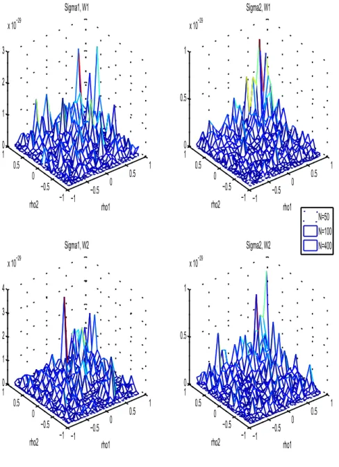
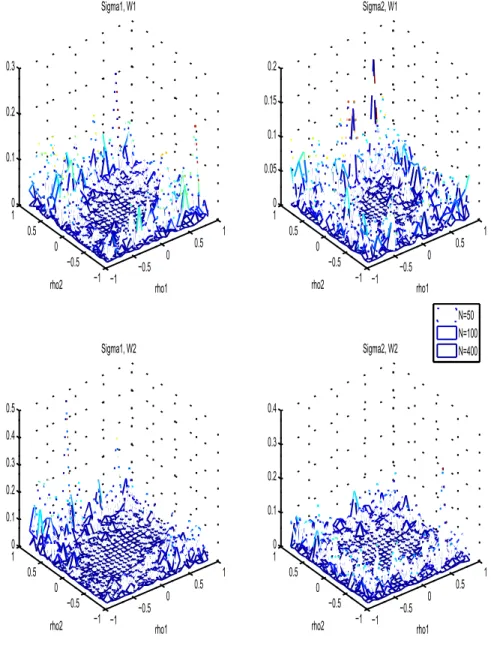
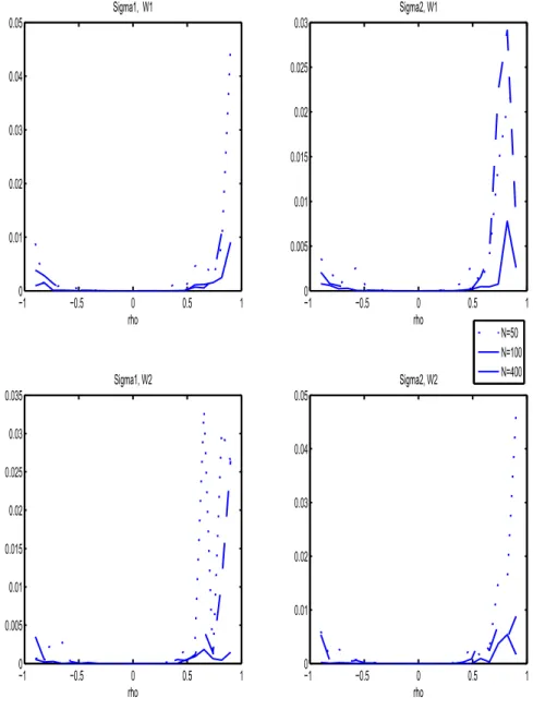
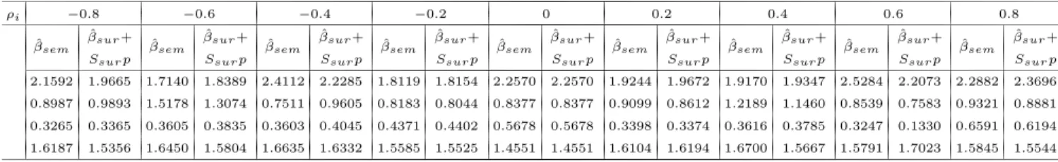
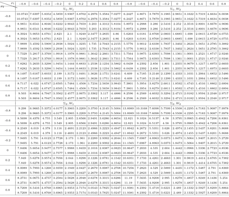
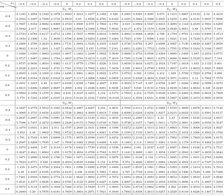
4 Simulation study: how good are Taylor approximations of GLS estimates?
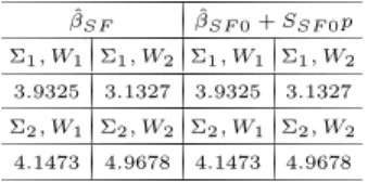
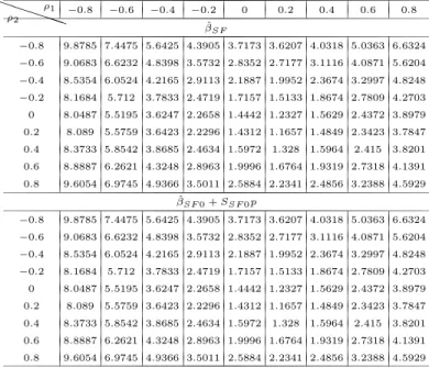
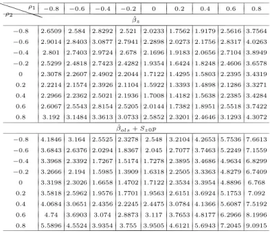
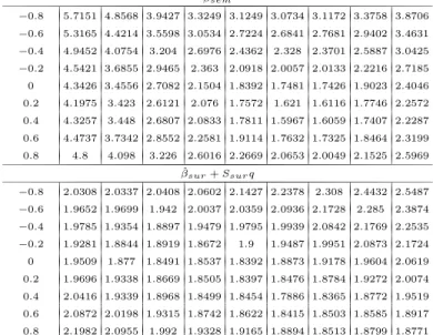
In this section, we use simulated data to compute the (generalized) least squares GLS estimates and their corresponding first order approximations, that were given in Theorems 2, 4, 7 and 9. We set the dimension of the panel system to T = 2, the number of observations to N = 50, 100, 400, and then I
N Tas an NT
×NT identity matrix, D
ρ= diag(ρ
1, ρ
2), and D
θ= diag(θ
1, θ
2). We set p = (ρ
1, ρ
2)
′= (0.2, 0.15)
′for Theorems 2 and 4, q = (θ
1, θ
2)
′= (0.1, 0.3)
′for Theorem 7, and θ = 0.3 for Theorem 9.
14
Two regressors X are drawn randomly from two T
×2 matrices of uniformly distributed random numbers from a uniform distribution U[0, 1]. We fix the regression coefficient values as β
1= (1, 2) and β
2= (0.5, 1.5).
We choose two neighborhood matrices W
Nas follows:
W
1=
0 0.5 0.5 0
· · ·0 0.5 0 0.5 0
· · ·0 0 0.5 0 0.5
· · ·0 ...
· · ·. .. ... ... ...
0
· · ·0 0.5 0 0.5 0
· · ·0 0.5 0.5 0
, W
2=
0 1 0 0
· · ·0 0.5 0 0.5 0
· · ·0 0 0.5 0 0.5
· · ·0 ...
· · ·. .. ... ... ...
0
· · ·0 0.5 0 0.5 0
· · ·0 0 1 0
(44)
We generate the error terms in e from a bivariate normal distribution N[0, Σ]
with mean 0 and covariance matrix Σ. The following two choices of Σ have been used, the first being the uncorrelated case and the second being the correlated:
Σ
1=
0.5 0 0 0.4
, Σ
2=
0.5 0.3 0.3 0.4