Location Models and their Cell Phone Applications Seminar Presentation Summary, Gabor Cselle, June 14, 2005 Advisor: Christian Frank

(1)

Location Models and their Cell Phone Applications

Seminar Presentation Summary, Gabor Cselle, June 14, 2005 Advisor: Christian Frank

Overview

In this article, we cover a range of topics related to the emerging uses of locational information on cellular phones, including location models, location inference, and resulting social and privacy-related issues. The first section presents a selection of models for identifying and de- scribing properties of location. In the following section, we examine a method to create location models on cell phones based solely on data about cell phone tower switches, and com- pletely without an underlying geographical database. Once location is uniquely identified and data about the current location of persons is recorded, we can infer facts about human behavior and social structure. We will examine the results of such a study in the third section and discuss privacy aspects.

1 An Introduction to Location Models

Location models define data structures in which we can store geographic information. For example, imagine an office building with two wings, and, spanning these wings, several floors with offices. The user of an information system may ask different kinds of questions, most of which will fall into one of these classes:

• Position queries: "Where am I?". The result should be the current position of the user in the model representation.

• Nearest neighbor queries: "Where is the next printer?". Based on a set of locations having some property that is stored in the model, find the nearest to a given location.

• Navigation queries: "How do I get to room C 42?". These queries should yield not a single answer, but a route of locations to follow.

• Range queries: "What printers are there on floor C?". Find a set of locations inside a bigger, containing location.

Position queries should be easy to answer in any representation. However, the other queries have more advanced requirements:

• Nearest neighbor queries. To be able to compare different possible locations and find the nearest one, we need a notion of distance.

• Navigation queries: Before we can run any route-finding algorithms, we need to understand which locations are connected to one another. Therefore, we need a notion of connectedness. In an office building, the individual locations would be rooms, and connections would be the doors between them.

• Range queries: To understand which locations are physically inside another, larger location, we need a notion of containment.

The following sections will present a number of location models and evaluate how well they fit these requirements. The challenge is to support all these notions so we can answer all possible query types quickly and efficiently.

1.1 Why Geocoordinates aren't Enough

Possibly the simplest way to express location is the approach used by GPS: It maps every location on planet Earth to latitude, longitude, and height coordinates. Still, simply listing coordinates often isn't enough.

First of all, No information is given about the position's properties. Knowing that you're at

(2)

you are at home or work. Also, based on coordinates, it is impossible to deduce information about connectedness and containment. Similarly, distance measurements can only be done by giving the Euclidean 3D-distance between two coordinates. In buildings or streets, this is just a lower bound: You have to walk through doors connecting rooms or follow the street layout instead of going in a straight line.

1.2 Symbolic Location Models

Symbolic models identify locations using names, not coordinates. Often, a range of coordinates (e.g. all coordinates in a building) is grouped into a single symbolic location.

When converting 3D space into a symbolic model, we choose the smallest unit of space we want to be able to represent. For our office building example, this would be a single room.

Each of these units gets assigned a node in a graph or an element in a set.

We now take up the challenge given above: We try to find a way to arrange these graphs or sets so all notions are supported and all queries can be answered.

The models presented were taken from [1]. Only the most important models are discussed.

1.2.1 Hierarchical Models

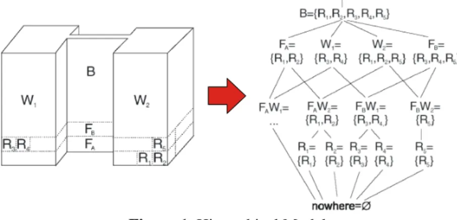
These models are based on contained-in relations. In our two-wing office building example above, each room is contained in both a floor and a wing.

Figure 1. Hierarchical Models

In hierarchical models, we create a set L for each unit of space: One for each room, floor, wing, and building. For overlapping sets (here, the floors' sets overlap the wings' sets), we need to create a set for every combination of them.

From these sets, we can create a lattice – a tree in which elements can have more than one parent, as illustrated in figure 1 – with the property:

A location l1 is an ancestor of a location l2 if l2 is spatially contained in l1.

How well does these models meet our requirements? To answer this question, we should evaluate what notions are supported by this type of location models.

Clearly, these models are great for containment queries. This relationship is modeled directly by the lattice.

On the other hand, The model does not have a good representation of distance. We can only make educated guesses with a simple observation: Given three locations l1, l2, l3∈L. If l1 and l2's least common ancestor is closer than l1's and l3's least common ancestor, then we can pre- sume that l1 and l2 are physically closer to each other than l1 and l3. For instance, we can guess that R1 and R2 with common ancestor FAW2 are closer to each other than R1 and R5 with least common ancestor FB.

Similarly, connectedness queries are not well-supported. Again, we can make an educated guess by saying that two locations that have a common ancestor are often connected.

(3)

1.2.2 Graph-based Models

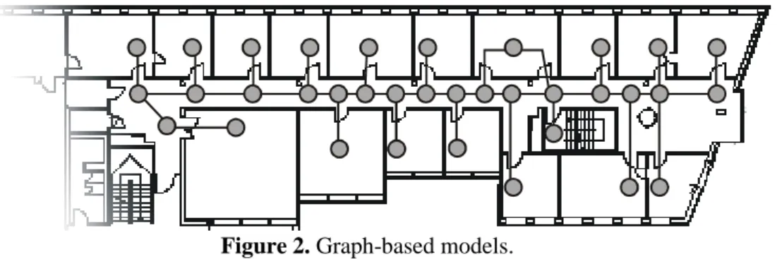
A simpler idea than the hierarchical model is the straightforward creation of a graph of locations. In the graph, vertices represent locations, while edges represent connections between the locations. Edges may be weighted to model distances.

Figure 2. Graph-based models.

This type of model excels in supporting the notions of distance and connectedness. The latter is supported directly, as connections correspond to edges. Distances can also be determined easily: By finding the shortest path (with one of the common algorithms), and adding up costs along it, we can find an almost perfect measure of distance between two locations.

Still, containment queries are difficult. For example, when a given room is known to be on floor C, we could guess that rooms that are a maximum distance of 2 away in the graph are on the same floor. But we can't be sure: one of the vertices close by might easily represent a flight of stairs.

1.2.3 Graph- and Set-Based Models

We will now combine the ideas from the preceding two models: We put the connection graph's vertices into sets identifying related locations.

For example, all vertices representing rooms on floor C would now go into a common set. In addition, by allowing sets to overlap, we can even model the fact that floors A and C are both in building a. This is illustrated in figure 3.

Figure 3. Graph- and set-based models

Obviously, we preserve all advantages of graph-based models: the notions of distance and connectedness are still well-supported. As an improvement, containment queries are much easier. All we need to do is perform membership tests on sets.

1.2.4 Subspace Models

Further adding to graph- and set-based models, we attach a geographic extent to each set:

Each set receives a coordinate system with a given origin. Additionally, vertices could store their coordinates (or even their own coordinate system with all coordinates of the room's cor- ners), relative to the origin. Figure 4 shows an example of this.

(4)

Figure 4. Subspace models

The supported notions are on-par with the graph- and set-based models, as we have been simply enhancing that type of model. Still, by adding the coordinate systems and position data, we can estimate the position of locations in space, which is important for applications that need more precise positioning.

1.3 Power Comes at A Price

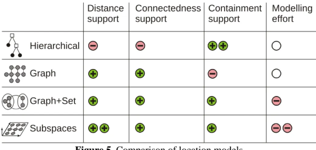
Figure 5 summarizes properties of the location models we have seen. Hierarchical models were optimized for answering containment queries and could only be used for educated guesses about distance and connectedness. Graphs, on the other hand, could easily answer questions about distance or connections, but offered little information about containment.

Combining the previous two approaches, graph- and set-based models gave us good answers to all questions. Subspace models added 3D information and are able to give even better measurements of distance on a sub-location level.

Throughout this section, we have been consistently increasing the complexity of our location models. However, we never mentioned the cost of such creating the model. Clearly, creating hierarchies of rooms, marking connections between them, or measuring their positions in space may require some effort and manual data entry.

Distance Connectedness Containment Modelling support support support effort Hierarchical

Graph Graph+Set Subspaces

Figure 5. Comparison of location models

Location data is useful for applications ranging from car navigation to marketing analyses.

For almost all applications, this data is collected by a commercial company, formatted accord- ing to a storage model, and made available to the user via an on-line database or on perma- nent storage (e.g. on DVDs). For cell phones, such data is not available or the data volume is too big. Still, based on cell tower records, we can infer location data on the phone itself, as shown in the next section.

(5)

2 Automatic Location Identification on Cell Phones

Every cell phone user has favorite locations where he spends a large proportion of his time.

For a student, these could be "home" and "university". Clearly, these are symbolic locations:

A range of 3D space is associated with a name.

For many cell phone applications, knowing which location the user is currently at would be useful. For instance, differentiating between "home" and "university" alone would be practi- cal for setting the current cell phone profile – during lectures, it is often advantageous to have the ring tone turned off. Including the current location in SMS messages to friends could help facilitate social meetings. But how can the current location be determined?

Systems like PlaceLab [4] try to estimate the current coordinates of a user by comparing the set of currently visible cell towers and 802.11 / Bluetooth devices with entries in a database.

But such data may not be available for the user's favorite locations. Also, each user's favorite locations are different: For example, everyone has a different "home" location.

The authors of [2] present an algorithm for automatically inferring the user's favorite locations. It is based on cell tower IDs only and does not require a database. While favorite locations are detected automatically, they need to be named manually by the user. This algorithm has actually been implemented on cell phones, thereby introducing some simplifications to the scheme presented here.

2.1 Problems with Input

The input data comes from software that is installed on the cell phone: It records changes of the primary cell tower. The primary cell tower is the one which the phone is currently logged on to and which would be used to handle calls.

Unfortunately, it is not possible to simply treat each cell tower as one location. There is no one-to-one correspondence between a physical location and the cell used by a phone, e.g., due to changing radio interference:

• Areas of cells can overlap, so that several cells may be seen in a single location.

• The overlap of cells and radio signal shadows can cause cells to be non-contiguous areas.

• Cells can be very large in the countryside or small in urban areas.

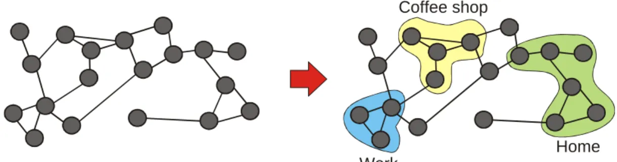
Our goal now is to group GSM cells into sets representing favorite locations. Each favorite location should correspond to a physical location where the user spends a lot of time (Fig. 6r).

Essentially, we're building a graph- and set-based location model, with the sets representing groups of cell towers whose reception indicates being at a favorite location.

To identify cells that are close to each other, the authors first create a "cell graph" (Fig. 6l). Its vertices are the observed GSM cells. Edges between two GSM cells exist if we observed a transition between them.

Home Work

Coffee shop

Figure 6. Cell graph and favorite locations we would like to obtain.

(6)

2.2 Steps to Identify Favorite Locations

When reception oscillates back and forth between a number of cell towers, this often means that multiple cell towers are in range at a location, not that the user is running back and forth between them. Therefore, subsets of the cell graph where oscillations are isolated and put into

"clusters". They must satisfy these properties:

1. The cells form a subgraph of diameter at most 2 in the cell graph.

2. The average time spent visiting a cluster is larger that the sum of individual visit times. This is fulfilled only when the user oscillates between cells in the cluster.

3. Any proper subset of the subgraph does not satisfy condition 2.

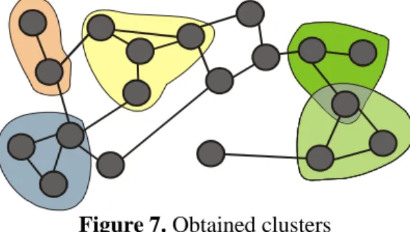
Figure 7. Obtained clusters

All locations that can later become favorite locations are then put into a candidate location set C. It contains the smallest reliably distinguishable locations in GSM cell data:

• All merged clusters (as seen in figure 7, clusters can overlap)

• All individual vertices not contained in clusters

But how do we know which locations are favorites, i.e. locations that the user spends a major- ity of time in? For this, weighted time spent in each candidate location is calculated:

0

( ) ( ) d

now

t

t t

C t

time C =

∫

at t r ⁻ t

Here, time is measured in days. The indicator function atC(t) is 1 if user is location L at time t, and 0 else. An exponential weighting of time is introduced with r^tnow-t; it makes stays at a location in the past less important than recent visits. The aging factor r is usually set to 0.95, so that r^tnow-t equals 0.25 for visits that occurred 14 days ago.

Finally, we identify the set F of favorite locations. It consists of a minimal set of locations that cover fraction p of all weighted time:

0

' '

arg min | ' |: ( ) d

now now

t

t t

F C F t

F F time C p r ⁻ t

⊆ ∈

 

 

=  ≥ 

 



∑ ∫



C

Here, 0 < p ≤ 1 defines how large a proportion of the total weighted time the bases must have.

In other words, favorite locations are the minimal set of locations in which the user spends proportion p of his total time, taking into account the weighting of time.

2.3 Example Results

The experimental results given in [2] list favorite locations for one of the researchers, who carried the cell phone around for 200 days. The method seems to identify all stable, recurring locations of everyday life (like work, home, leisure, friends and family) as well as more tran- sient locations on trips (like accommodation in different places).

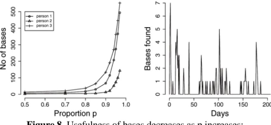
One issue is the required proportion of the time spent in bases. Reasonable results are achieved with p = 0.8. As p is increased, many bases are discovered which are not necessarily meaningful (Figure 8).

(7)

Figure 8. Usefulness of bases decreases as p increases;

number bases to be named manually per day

The right side of Fig. 8 shows that after an early rush, there only few days on which more than two bases need to be named manually. Thus, the manual naming of bases should not be an issue.

2.4 Possible Applications

The authors of [4] describe an application where cell phone users can send "location requests"

to each other via an SMS-based protocol. The user can then select his present location from a list of likely current locations, and send it back via SMS. This method could improve the de- tection quality of the current location.

A real-world example is dodgeball.com. A user registers with the website and lists her friends. To "check in" to the system when at a bar, she types an SMS message with her user- name and name of the bar and sends it to Dodgeball. Whenever a friend "checks in" at a location within a 10 street block radius, the application will send both the friend and her an SMS, encouraging to meet each other.

This application could be significantly improved if the all bars' locations could be identified as bases with a variant of the method we described: Hired scouts could walk through all the bars and record cell tower transitions, yielding clusters as described before. The merged clusters would then manually be assigned a bar name. This would make it possible to offer automatic "check-ins", without manual intervention. This could be coupled with a sign in/out mechanism to turn automatic check-ins on and off, thereby alleviating privacy concerns.

3 Detecting Human Behavior Patterns

Once locations are uniquely identified for each user, we are free to experiment. As a conclusion to this article, we will present the results of a field study [3] where a large amount of cell phone data was gathered from 100 cell phones over months. The study included 75 students and faculty of the MIT Media Lab, and 25 students from the neighboring business school.

Bluetooth beacons were installed throughout the buildings in which the participants would spend their time during work hours. The phones scanned their environment for Bluetooth beacons once every five minutes. Since device discovery works only within 10 m, their position could be identified to be within this 10 m radius.

By analyzing the data in different ways, we can recognize some usual human behavior patterns.

3.1 Results

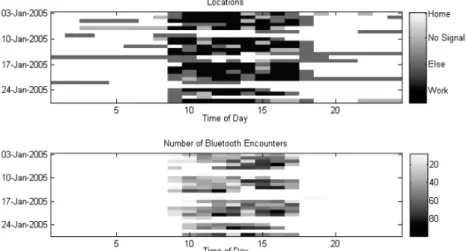
Figure 9 gives the daily transition patterns and Bluetooth encounters for a 'low-entropy' user and the inferred location. A low-entropy user is one whose days follow similar patterns.

Weekends can clearly be differentiated from weekdays.

(8)

Figure 9. Location transition patterns for a low-entropy user

For the study, test subjects gave a list of friends and acquaintances who were also test subjects. This yielded a friendship graph as shown in figure 10, on the left. When constructing a graph of encounters that occurred daily, the authors obtained the graph on the right. The two graphs share a similar structure.

Media Lab students

Business school students

Figure 10. Friendship graph vs. proximity graph

The tendency of humans to be stay physically close to their friends is reflected also in Figure 11. It lists proximity frequencies depending on time, weekday and relationship. More time is spent with friends than with acquaintances, especially at off-work hours.

Friend

Aquaintance

Figure 11. Time spent with friends vs. acquaintances.

(9)

This study showed how human behavior is reflected in cell phone data. It also shows how important the privacy and confidentiality of such data is: Such an experiment cannot be carried out without the consent of participants. Their incentive to participate was, of course, receiving a brand-new cell phone.

Conclusion

In this article, we presented several topics:

1. How physical locations can be modeled efficiently,

2. how mobile phones can infer location models autonomously, without the need for an underlying database, and

3. how location tracking data can be used for analyzing human behavior.

The last two points require further discussion.

In section 2, we demonstrated that mobile phones can identify important locations for the user. This has several uses: Many applications can be imagined that make use of the current position of the owner: Turning off the ringing sound at work, or looking up the closest pizzeria. The advantage of the presented method is that it can identify locations we spend a lot of time in, and do so without a location database.

This is a clear benefit: while mapping approaches such as PlaceLab exist, the entire globe has so far not been mapped out by 'war drivers', so there would always be areas without coverage.

Also, we would either need to contact a central database wirelessly to retrieve information about the surroundings, or have a periodically updated database stored in the cell phone at all times.

The author believes that these barriers will vanish: Via always-on services, e.g. through GPRS, it is easy to load contents of a database on-the-go. Also, storage capacities of cell phones have been increasing: Current models come equipped with up to 512 MB of storage.

Since it's possible to store the all road maps of Central Europe on a 4.7 GB DVD for cars, it should also be possible to have large amounts of beacon information stored on cell phones.

A great inhibitor, however, is the need to spend a large amount of time in the locations to be identified. Mostly, when a user wants locational information, such as positional queries ("where am I"?) or nearest neighbor queries ("where is the next pizzeria"), he asks these about locations he has not yet been to or does not visit often. These locations would not be detected as favorite locations in the presented algorithm.

Therefore, the author believes that online location identification, while useful for the time being, may be replaced by database-centered applications in the long run.

The study we saw in the third section showed us – among other things – how much we should be worried about privacy. Clearly, data about personal behavior and the social network can be generated from cell phone data with surprising accuracy.

Some applications are imaginable: A phone company collects this information and finds out who your friends are. It could then share this information with the user's cell phone, and makes sure you have all of your friends' cell phone numbers.

However, it seems that the weight of lost privacy far outweighs the benefits. Instead, the author believes that phone companies should be kept from spying and analyzing their customers this way. However, any limitations shouldn't be too far-reaching, as making locational information available on cell phones will have many exciting and useful applications.

(10)

References

[1] Becker C, Dürr F: "On Location Models for Ubiquitous Computing"
Personal and Ubiquitous Computing, Volume 9, Issue 1 (Jan 2005) [2] Laasonen K, Raento M, Toivonen H:
"Adaptive On-Device Location Recognition"
Pervasive 2004, Vienna, Austria
[3] Eagle N, Pentland A: "Reality Mining: Sending Complex Social Systems"
Personal and Ubiquitous Computing, to appear: June 2005
[4] Smith I, et al: "Social Disclosure of Place: From Location Technology to Communication Practices", Pervasive 2005
[5] LaMarca A, et al.: "Place Lab: Device Positioning Using Radio Beacons in the Wild", Pervasive 2005