Symmetry breaking in a bulk-surface reaction-diffusion
model for signaling networks
Andreas R¨ atz and Matthias R¨ oger
Preprint 2013-07 Mai 2013
Fakult¨at f¨ur Mathematik
Technische Universit¨at Dortmund Vogelpothsweg 87
44227 Dortmund tu-dortmund.de/MathPreprints
MODEL FOR SIGNALING NETWORKS
ANDREAS R ¨ATZ AND MATTHIAS R ¨OGER
Abstract. Signaling molecules play an important role for many cellular functions. We investi- gate here a general system of two membrane reaction–diffusion equations coupled to a diffusion equation inside the cell by a Robin-type boundary condition and a flux term in the membrane equations. A specific model of this form was recently proposed by the authors for the GTPase cycle in cells. We investigate here a putative role of diffusive instabilities in cell polarization. By a linearized stability analysis we identify two different mechanisms. The first resembles a classi- cal Turing instability for the membrane subsystem and requires (unrealistically) large differences in the lateral diffusion of activator and substrate. The second possibility on the other hand is induced by the difference in cytosolic and lateral diffusion and appears much more realistic.
We complement our theoretical analysis by numerical simulations that confirm the new stabil- ity mechanism and allow to investigate the evolution beyond the regime where the linearization applies.
1. Introduction
In numerous biological processes the emergence and maintenance of polarized states in the form of heterogeneous distributions of chemical substances (proteins, lipids) is essential. Such symmetry breaking for example precedes the formation of buds in yeast cells, determines di- rections of movement, or mediates differentiation and development of cells. Polarized states in biological cells often arise in response to external signals, typically from the outer cell membrane.
Transport processes and interacting networks of diffusing and reacting substances both within the cell and on the cell membrane then amplify and process such signals. The distribution of small GTPase molecules in eukaryotic cells presents one example of a complex system with polarization and motivates the present paper. Such molecules can be in an active and in an inactive state.
Activation and deactivation typically occurs at the cell membrane and is catalyzed by specific enzymes. In addition to the activation-deactivation cycle GTPase molecules (in its inactive form) shuttle between the membrane and the cytosol, i.e. the inner volume of the cell, by attachment to and detachment from the membrane. These properties induce the specific form of a coupled volume (bulk) and surface reaction–diffusion system. The goal here is to investigate a possible contribution of diffusive instabilities to cell polarization in such coupled systems.
Different deterministic continuous models have been used to investigate polarization of cells (see for example the review [8]). We consider here a particular class of models that takes the form of a reaction-diffusion system on the membrane coupled to a diffusion process in the interior of the cell. This model has been introduced in [17] where a reduction to a non-local reaction-diffusion system, involving only membrane variables, has been investigated. A key question in such systems is whether a Turing-type mechanism may contribute to the polarization of cells, with activated GTPase and inactive GTPase representing self-activator and substrate, respectively. Turing- type instabilities however require large differences in the diffusion constants for activator and substrate (or inhibitor). The lateral diffusion on the membrane for active and inactive GTPase on the other hand is in general of comparable size and therefore a Turing instability appears at
Date: May 27, 2013.
2000Mathematics Subject Classification. 92C37,35K57,35Q92.
Key words and phrases. Reaction-diffusion systems, PDEs on surfaces, Turing instability, numerical simulations of reaction-diffusion systems.
1
first glance unrealistic. On the other hand, cytosolic diffusion in cells is typically much faster than lateral diffusion and might induce the necessary difference in diffusion. It is therefore tempting to hypothesize that in such coupled 2D and 3D reaction–diffusion systems diffusive instabilities can in fact contribute to cell polarization.
We will in the following represent the cytosolic volume and the membrane of a cell by a bounded, connected, open domainB ⊂R3in space and its two-dimensional boundary Γ :=∂Brespectively.
We assume that Γ is given by a smooth, closed surface and denote byν the outer unit normal ofB on Γ. Further we fix a time interval of observationI := [0, T]⊂Rand consider smooth functions V :B ×I → R, u, v: Γ×I → R (representing the cytosolic inactive, membrane-bound active, and membrane-bound inactive GTPase, respectively) that satisfy the coupled reaction–diffusion system (stated in a non-dimensional form)
∂tV =D∆V in B×I, (1.1)
∂tu= ∆Γu+γf(u, v) on Γ×I, (1.2)
∂tv=d∆Γv+γ(−f(u, v) +q(u, v, V)) on Γ×I, (1.3)
−D∇V ·ν=γq(u, v, V) on Γ×I. (1.4)
Here f and g represent the activation/inactivation processes and q describes attach- ment/detachment at the membrane. In the appendix we present as specific example the mathe- matical model for the GTPase cycle from [17] with explicit choices for f and q that we also use in our numerical simulations below. The parameterγ >0 is a non-dimensional parameter that is related to the spatial scale of the cell. The coupling of bulk and surface processes in (1.1)–(1.4) is given in form of a Robin-type boundary condition. The system is complemented by initial conditions at time t= 0,
V(·,0) = V0, v(·,0) = v0, u(·,0) = u0, V0 : B → R, v0, u0 : Γ → R.
We remark that the system (1.1)–(1.4) automatically satisfies conservation of total mass, i.e.
M(t) :=
Z
B
V(x, t) dx+ Z
Γ
(u+v)(x, t) dσ(x) = const, where dσ denotes integration with respect to the surface area measure.
In this contribution we investigate the possibility of diffusive instabilities for systems of the form (1.1)–(1.4). We present a linear stability analysis and numerical simulations. We find two possible scenarios for a diffusive instability of spatially homogeneous stationary states. The first needs large differences in lateral diffusion foruand v(i.e. a coefficient d1) and resembles a classical Turing instability in theu, vvariables. The second mechanism on the other hand does also occur for equal lateral diffusion constantsd= 1 and is rather based on the different diffusion constants foruandV and therefore on the coupling of bulk and surface equations. As cytosolic diffusion is typically by a factor hundred faster than lateral diffusion, this scenario is much more realistic in the application to signaling networks. In Section 3 we compare the stability of the full system to its reduction in the formal limitD→ ∞. The latter leads to a non-local two-variable system on the membrane that has been analyzed in [17] (see also [19]). There we have only covered the first more
‘classical’ instability mechanism and have not included a complete characterization of diffusive instabilities. Here we show that – in coincidence with the case D <∞ – we again have the same alternative scenarios for diffusive instabilities. Some specific properties of the second instability mechanism are easier to characterize in the reduction. In particular we find that the second scenario is different from a standard Turing-type instability as in this case the concentration of activated GTPase in a single spot (most typical in most examples of cell polarization) is always preferred independent of variations in the parameter values. This robustness makes the second instability mechanism an even more attractive explanation for polarization. In Section 4 we present numerical simulations for specific versions both of the full system (1.1)–(1.4) and of the
reduced system. The simulations confirm the instability criteria derived for the linearised system and allow to investigate the time-evolution after the onset of heterogeneities and beyond the regime governed by the linearization. It turns out that even for simple choices of the constitutive relationsf andqthe system exhibits a rich behavior. In the final Section 6 we discuss the results of the paper and in particular comment on the term ‘diffuse instability’ in the present context and with respect to the second instability mechanism.
The most specific property of the model considered here is the coupling of bulk and surface reaction–diffusion systems. Such coupled systems often arise in cell biology where enzymatic processes on intracellular membranes play a role, see [15] and the references therein. Surface–
bulk reaction–diffusion or convection–diffusion systems also arise in the modeling of surfactants on two-fluid interfaces [20]. Coupled surface–bulk systems have been studied intensively over the last decades by numerical simulations, see for example [13, 20, 6, 15, 3] and the references therein.
In [13] a model that is similar to ours and that describes a two-variable diffusion system in a volume coupled to a reaction system on the boundary has been studied. Here the authors provide numerical simulations and a linear stability analysis. They show the existence of Turing instabilities in their model, even for equal bulk diffusion constants. The main difference to our model is that in [13] both activator and substrate diffuse in the bulk and that no diffusion on the membrane surface is considered.
2. Stability Analysis For the Full System
We consider in the following the spatially coupled reaction–diffusion system (1.1)–(1.4) for spherical cell shapes and investigate the possibility of diffusive instabilities of a homogeneous stationary state. Because of the different domains of definition of V and u, v we cannot apply standard conditions for (in)stability and therefore will derive appropriate criteria in this section.
Similar to a classical Turing instability we consider a spatially homogeneous stationary state and require that this state is (a) stable against perturbations of the membrane quantities u, v that are spatially homogeneous on the membrane and perturbations of the bulk variable V that are radially symmetric (this additional restriction follows already by the first) and (b) unstable with respect to general perturbations. Such property represents a diffusive instability and a symmetry breaking in the sense that the radially symmetric evolution loses its stability as it approaches such a stationary point.
For the constitutive relationsf, q we assume that
∂vf ≥ 0, ∂vq ≤ 0, ∂vq ≤ ∂uq, ∂Vq ≥ 0, (2.1) which are for the application to the GTPase cycle natural conditions with respect to the interpre- tation off as activation rate andq as the flux induced by ad- and desorption of GTPase at the membrane. As we are interested in symmetry breaking we consider in the following a spatially homogeneous stationary state (u∗, v∗, V∗) ∈ R3+ := {(x1, x2, x3) ∈ R3 : xi > 0, i = 1,2,3} of (1.1)–(1.4), which is equivalent to the conditions
f(u∗, v∗) = 0, (2.2)
q(u∗, v∗, V∗) = 0. (2.3)
For convenience we introduce the following notation, fu := ∂uf(u∗, v∗), fv := ∂vf(u∗, v∗),
qu := ∂uq(u∗, v∗, V∗), qv := ∂vq(u∗, v∗, V∗), qV := ∂Vq(u∗, v∗, V∗). (2.4) We assume that in (V∗, u∗, v∗) we have strict inequalities
fv > 0, qv < 0, qV > 0, (2.5)
The linearization of (1.1)–(1.4) in (V∗, u∗, v∗) is given by the system
∂tV =D∆V in B×I, (2.6)
∂tu= ∆Γu+γ fuu+fvv
on Γ×I, (2.7)
∂tv=d∆Γv+γ (−fu+qu)u+ (−fv+qv)v+qVV
on Γ×I, (2.8)
−D∇V ·ν=γ quu+qvv+qVV
on Γ×I (2.9) for unknowns V : B ×R → R, u, v : Γ×R → R, together with a constraint on the initial conditions, due to the mass conservation property,
Z
B
V(x,0) dx+ Z
Γ
u(x,0) +v(x,0)
dσ(x) = 0. (2.10)
In the following we assume that no inner membranes are present and assume a spherical shape of the cell, i.e. we chooseB =B1(0) and Γ =∂B =S2. This allows in the subsequent stability analysis to use separated variables: we introduce polar coordinates and representx∈Basx=ry withy∈S2, r∈[0,1]. We further fix an orthonormal basis{ϕlm}l∈N0,m∈Z,|m|≤lofL2(Γ) given by spherical harmonics with
−∆Γϕlm = l(l+ 1)ϕlm on Γ (2.11)
and remark that ϕ00 is constant on Γ. We then consider the following ansatz for solution of the linearized system (2.6)–(2.9),
u(y, t) = X
l∈N0,m∈Z,|m|≤l
ulm(t)ϕlm(y), (2.12)
v(y, t) = X
l∈N0,m∈Z,|m|≤l
vlm(t)ϕlm(y), (2.13)
V(ry, t) = X
l∈N0,m∈Z,|m|≤l
Vlm(t)ψlm(r)ϕlm(y), (2.14) with ulm, vlm, Vlm :R → R, ψlm : [0,1]→ R, y ∈Γ,0≤r ≤1 (for a similar approach see [13]).
We deduce from (2.6)–(2.9), by taking theL2(Γ) scalar product withϕlm,
u0lm =−l(l+ 1)ulm+γ(fuulm+fvvlm), (2.15) vlm0 =−dl(l+ 1)vlm+γ
(−fu+qu)ulm+ (−fv+qv)vlm+qVψlm(1)Vlm
, (2.16) Vlm0 (t)ψlm(r) =DVlm(t)
ψlm00 (r) +2
rψlm0 (r)− 1
r2l(l+ 1)ψlm(r)
, (2.17)
−DVlmψlm0 (1) =γ(quulm+qvvlm+qVψlm(1)Vlm). (2.18) From (2.17) we obtain that
Vlm(t) = ¯Blmeωlmt, B¯lm∈R, ωlm ∈R, (2.19) and Vlm is either identically zero or does nowhere vanish.
In the following we first restrict ourselves to the caseVlm6= 0. We deduce that 0 = r2ψlm00 (r) + 2rψlm0 (r)−
l(l+ 1) + ωlm D r2
ψlm(r). (2.20)
If in additionωlm >0, the latter equation implies that ψlm(r) = αlmil
rωlm D r
, αlm ∈R, (2.21)
il(r) = rπ
2rIl+1 2(r),
whereIl+1
2 denotes the respective modified Bessel functions of first kind.
In the caseωlm= 0 we obtain instead
ψlm(r) = αlmrl, αlm∈R. (2.22) We derive from (2.15), (2.16), (2.19) and (2.18) the linear ODE system
u0lm = −l(l+ 1) +γfu
ulm+γfvvlm, (2.23)
vlm0 =−γfuulm− dl(l+ 1) +γfv
vlm−Dψlm0 (1)Vlm, (2.24)
Vlm0 =ωlmVlm, (2.25)
coupled to an algebraic equation
0 =γ(quulm+qvvlm) + γqVψlm(1) +Dψ0lm(1)
Vlm, (2.26)
that determines in the case Vlm 6= 0 together with (2.21) the value of ωlm. The linear stability analysis then reduces to an analysis of the eigenvalue equation coupled to an algebraic condition.
We obtain that an eigenvalueω with nonnegative real part exists if and only if firstω=ωlm∈R+0
and second ωlm satisfies 0 =! Gl(ωlm)
:= γqV
ω2lm+ (d+ 1)l(l+ 1) + (−fu+fv)γ
ωlm+dl2(l+ 1)2+γl(l+ 1)(−dfu+fv) +κD,l(ωlm)
ω2lm+ (d+ 1)l(l+ 1) + (−fu+fv)γ ωlm+ +dl2(l+ 1)2+γl(l+ 1)(−dfu+fv) +κD,l(ωlm)
−γqv l(l+ 1) +ωlm
+γ2 fuqv−fvqu
(2.27) with
κD,l(ω) := Dψlm0 (1) ψlm(1) = D
ri0l(r) il(r)
r=√
ω D
, (2.28)
where the last equality follows for ω > 0 from (2.21) and for ωlm = 0 from (2.22) and (2.38) below.
In the caseVlm= 0, which is equivalent to ¯Blm = 0, the system (2.15)–(2.18) is overdetermined.
We obtain that the parameters have to satisfy the equation (d−1)l(l+ 1)qu = γ(−fuqv+fvqu) 1
qv
(qu−qv) (2.29)
and that under this condition any eigenvalue ω corresponding to the linearized system (2.15)–
(2.18) is given by
−quω = γ(−fuqv+fvqu) +dl(l+ 1)qu. (2.30) Due to the condition (2.29) the caseVlm= 0 is only relevant for a small – nowhere open – subset of the parameter space. Therefore this case cannot contribute to a robust mechanism.
2.1. Asymptotic stability with respect to spatially homogeneous perturbations. Here we would like to consider perturbations u, v, V of a stationary state (u∗, v∗, V∗) ∈R3+ such that the membrane quantities u, v are spatially homogeneous but V is allowed to be heterogeneous.
We would like to characterize the stability of our system under such perturbations. In the ansatz above the restriction to spatially homogeneous u, v means that ulm =vlm = 0 for all l≥1. By (2.24) and ψlm0 (1) > 0 (see for example [1, (10.51.5)], [16]) we deduce that alsoVlm = 0 for all l ≥ 1, and in particular that V is radially symmetric. It remains to study the condition (2.27) forl= 0.
Proposition 2.1. A necessary and sufficient condition for the stability of (1.1)–(1.4) in (u∗, v∗, V∗) under perturbations that are spatially homogeneous in the u, v variables is that
0 < 1
3(fuqv−fvqu) +qV(fv−fu). (2.31) In this case
fv > fu (2.32)
holds.
Proof. As remarked above we have to consider l = 0. We first restrict ourselves to the case V006= 0. Then the system (1.1)–(1.4) is linearly asymptotically stable in (u∗, v∗, V∗) if and only if
G0(ω) = γqV ω2+ (−fu+fv)γω
+κD,0(ω) ω2+ (−fu+fv)γω
−κD,0(ω) γqvω−γ2 fuqv−fvqu
(2.33)
has no zeroes in [0,∞). Let us first consider the case ω >0. For convenience we then rewrite κD,0(ω) = D
ri00(r) i0(r)
r=√ω
D
= ωκ˜ rω
D
,
˜
κ(r) := i00(r) ri0(r).
Explicit evaluation of ˜κ gives that ˜κ0 <0. In fact we have i0(r) = sinhr
r , i00(r) = rcoshr−sinhr
r2 ,
˜
κ(r) = rcoshr−sinhr r2sinhr , hence
˜
κ0(r)r3sinh2r = −r2+ 2 sinh2r−rsinhrcoshr
= −r2−1 + cosh 2r−r
2sinh 2r
= X
k≥2
1
(2k)!(2r)2k(1−k 2) < 0.
Furthermore we obtain
r→0limκ(r) =˜ 1
3, lim
r→∞˜κ(r) = 0. (2.34)
Forω >0 the equation G0(ω) = 0 is equivalent to 0 = ˜κ
rω D
ω2+γω(fv−fu−qv) +γ2(fuqv−fvqu)
+γqVω+γ2qV(fv−fu) =: ˜G0(ω).
(2.35) By (2.34) andqV >0 we deduce that limω→∞G˜0(ω) = +∞. Using (2.34) we evaluate
ω→0lim
G˜0(ω) = 1
3γ2(fuqv−fvqu) +γ2qV(fv−fu), and we obtain that
0 ≤ 1
3(fuqv−fvqu) +qV(fv−fu). (2.36) is a necessary condition for ˜G0 >0 on (0,∞).
Let us next consider the case ω = l = 0 which gives G0(0) = 0. In this case u, v, V are all constant and satisfy, by (2.7), (2.8) and (2.10),
0 = fuu+fvv, 0 = quu+qvv+qVV, 0 = 4π(u+v) +4π
3 V.
This system has a nontrivial solution if and only if 0 = 13(fuqv−fvqu) +qV(fv−fu). Together with (2.36) this property proves that (2.31) is necessary for the asserted stability.
From (2.31) we deduce that
0 < (fv−fu)(qV −1
3qv) +1
3(qv−qu)fv ≤ (fv−fu)(qV −1 3qv).
By (2.1) this implies (2.32) and in particular that (2.32) is necessary for ˜G0>0 on [0,∞).
We claim that (2.31) is also sufficient to exclude a nonnegative zero ofG0. Again, we consider forω >0
G˜0(ω) = ˜κ rω
D
ω2+γω(fv−fu−qv) +γ2(fuqv−fvqu)
+γqVω+γ2qV(fv−fu).
As (2.31) implies (2.32) we have by (2.5) thatfv −fu−qv >0 and qV(fv−fu)>0. If we now assume
fuqv−fvqu >0,
we immediately conclude ˜G0(ω)>0 for allω >0. If on the other hand fuqv−fvqu ≤0,
we remark that ˜κis decreasing, hence ˜κ≤ 13 on [0,∞) and therefore G˜0(ω)> γ2 1
3(fuqv−fvqu) +qV(fv−fu)
≥ 0
for all ω > 0, which proves the claim. We have already seen above that 06= 13(fuqv −fvqu) + qV(fv −fu) is sufficient to exclude that constant perturbations (u, v, V), corresponding to the case ω= 0, are solution of the linearized system.
It only remains to prove that (2.31) is sufficient to exclude an instability for l= 0 in the case V00 = 0. However, in this case by (2.29), (2.30) we have ω = 0 and we are in the case that (u, v, V) is constant, which is excluded by (2.31), as we have seen above.
2.2. Instability conditions. We next characterize instabilities of our system in a spatially ho- mogeneous stationary point (u∗, v∗, V∗) as above under general perturbations.
Theorem 2.2. Assume that (2.31)is satisfied and that
0 >(γqV +Dl) dl2(l+ 1)2+γl(l+ 1)(−dfu+fv)
−Dγqvl2(l+ 1) +Dlγ2(fuqv−fvqu) (2.37) holds in(u∗, v∗, V∗). Then the system (1.1)–(1.4)is linearly asymptotically unstable in(u∗, v∗, V∗).
If (2.31)and d= 1 hold then (2.37) is also necessary for an instability.
Proof. We again first restrict to the caseVlm 6= 0. Note that the right-hand side of (2.37) coincides with Gl(0) as defined in (2.27). In order to show the existence of an instability, we prove that
there is a positive zero ωlm >0 of Gl. The modified Bessel function of the first kind il have by [1, 10.52.1, 10.52.5], [16] the asymptotic expansions
il(r) ≈ 1
2rer asr → ∞, il(r) ≈ 1
(2l+ 1)!rl asr→0.
This implies
κD,l(ω) =D
ri0l(r) il(r)
r=√ω
D
→ Dl asω→0, (2.38)
and κD,l(ω)→ ∞ asω→ ∞ hence
ω→∞lim Gl(ω) = +∞.
We therefore obtain that (2.37) is sufficient to guarantee a solution ω > 0 of Gl(ω) = 0. It remains to prove that (2.37) is also necessary if d= 1 holds. We will need some information on the derivative of κD,l. We start by observing that by (2.28)
κ0D,l(ω) = h1 2r
ri0l(r) il(r)
0i
r=√
ω D
. By the definition ofil we compute
ri0l(r)
il(r) = −1
2+ rIl+1/20 (r) Il+1/2(r) .
By [5] however we know that the quotient on the right-hand side has strictly positive derivative on R+. This implies that alsoκ0D,l>0. Moreover, from [7, 12] we obtain
ri0l(r)
il(r) ≤l+ 1 3r2 which yields
κD,l(ω)≤lD+ 1
3ω=κD,l(0) +1
3ω (2.39)
for all ω >0.
This information implies by (2.27), (2.32), andd= 1 that Gl(ω) ≥ γqV
dl2(l+ 1)2+γl(l+ 1)(−dfu+fv) + (−fu+fv)γω +κD,l(ω)
dl2(l+ 1)2+γl(l+ 1)(−dfu+fv) +κD,l(ω)
−γqv l(l+ 1) +ωlm
+γ2 fuqv−fvqu
≥Gl(0) +γ2qV(fv−fu)ω+γ2 κD,l(ω)−κD,l(0)
(fuqv−fvqu). (2.40) In the case (fuqv −fvqu) > 0 this yields Gl(ω) ≥ Gl(0) for all ω > 0, as κD,l is increasing (see above). In the case (fuqv−fvqu)≤0 we obtain from (2.40) that
Gl(ω)
(2.31)
≥ Gl(0)−γ2(fuqv−fvqu) 1
3ω−κD,l(ω) +κD,l(0) (2.39)
≥ Gl(0).
for all ω > 0. From this we conclude that Gl(0) < 0 is also necessary for the existence of an instability with Vlm 6= 0.
It remains to consider the possibility that an instability with Vlm = 0 exists. In this case we obtain from (2.29) and d= 1 that−fuqv+fvqu = 0. But then (2.30) implies thatω ≤0.
Corollary 2.3. Assume (2.31). Then the instability condition (2.37) holds if the conditions of Case 1 or Case 2 below are satisfied and if D >0 is chosen sufficiently large.
• Case 1:
fuqv−fvqu ≥ 0, (2.41) dfu−fv+qv >0, (2.42) Q := (dfu−fv+qv)2−4d(fuqv−fvqu) >0, (2.43) and there exists anl∈Nwith
λ− < l(l+ 1)
γ < λ+, (2.44)
where
λ± = 1 2d
dfu−fv+qv±p Q
. (2.45)
• Case 2:
fuqv−fvqu < 0 (2.46)
and there exists anl∈Nwith
l(l+ 1)
γ < λ+, (2.47)
where λ+ is as defined in (2.45).
Proof. In order to evaluate (2.37) for D1 we consider the coefficient ofDl, that is
e := dl2(l+ 1)2+γl(l+ 1)(−dfu+fv−qv) +γ2(fuqv−fvqu). (2.48) In Case 1 the last term on the left-hand side is by (2.41) nonnegative and e <0 holds if and only if the conditions (2.42)–(2.44) are satisfied.
In Case 2 the last term on the left-hand side of (2.48) is negative and e < 0 holds if and only if the condition (2.47) is satisfied. Therefore e < 0 holds if and only if Case 1 or Case 2 are satisfied. We now observe that the term Dle becomes dominant in (2.37) for D 1 and we deduce from Theorem 2.2 that ife <0 then forDsufficiently large an instability exists.
Remark 2.4. (1) For d = 1 we deduce from Theorem 2.2 and (2.31), (2.37) that a diffusive instability exists if and only if
0 >(γqV +Dl) l2(l+ 1)2+γl(l+ 1)(−fu+fv)
−Dγqvl2(l+ 1) +Dlγ2(fuqv−fvqu) holds. By (2.32) we deduce that (2.46) is necessary and that only Case 2 is a possible scenario for an instability. By Corollary 2.3 this condition and (2.47) for anl∈Nare also sufficient to ensure, forD sufficiently large, an instability. In particular, ford= 1 there exist parameter values such that the system has a diffusive instability.
(2) Assume (2.31). Then we observe from (2.27) that perturbations in directions of eigenvectors ϕlm decay for all sufficiently largel∈N.
(3) Case 1 or Case 2 in Corollary 2.3 are sufficient but not necessary for an instability. A third case may arise for d 1 and D sufficiently small. In fact, even if the factor that multiplies κD,l(ω) in (2.27) is positive, this term might be dominated by the first line in (2.27), which becomes negative ifdfu−fv 1. As we are mostly interested ind= 1 we do not investigate this case further.
Remark 2.5. We finally would like to relate the distinction between Case 1 and Case 2 insta- bilities, given by the inequalities (2.41) and (2.46), to the stability properties of the zero lateral diffusion reduction of the full system (1.1)–(1.4). This reduction is given by choosingdu =dv= 0
in the dimensional formulation of our system, see (A.10) and (A.11) in the appendix and leads to the system
∂tV =D∆V in B×I, (2.49)
∂tu=γf(u, v) on Γ×I, (2.50)
∂tv=γ(−f(u, v) +q(u, v, V)) on Γ×I, (2.51)
−D∇V ·ν=γq(u, v, V) on Γ×I. (2.52)
An instability of the corresponding system is then characterized by the existence of a positive rootωlm of
0 = γqV ωlm2 + (−fu+fv)γωlm +κD,l(ωlm)
ωlm2 + (−fu+fv−qv)γωlm+γ2 fuqv−fvqu
(2.53) withκD,l as in (2.28). We therefore see that under the stability assumption (2.31) in Case 1, i.e.
if (2.41) holds, the system (2.49)–(2.52) is stable, whereas for Case 2, i.e. if (2.46) holds, the system is unstable forD1 andγ chosen large enough. This shows that the second instability mechanism is not induced by the membrane diffusion but rather by the cytosolic diffusion. See Section 6 for a further discussion.
3. Stability Analysis for the non-local reductionD→ ∞
By formally lettingD→ ∞in (1.1)–(1.4) one obtains the following reduced two-variable system
∂tu = ∆Γu+γf(u, v), (3.1)
∂tv = d∆Γv+γ(−f(u, v) +q(u, v, V[u+v])), (3.2) whereV[u+v] is the non-local functional
V[u+v] = Vinit−c Z
Γ
(u+v) dσ, (3.3)
with Vinit > 0 given and c := |B|1 . Note that Vinit is determined by the total mass of GTPase, which is constant in time. The system (3.1)–(3.3) has already been considered in [17] and has, compared to the fully coupled system, the advantage of having one fixed domain of definition (the membrane Γ). The remnant of the spatial coupling in the full system is the non-locality, introduced by the specific form ofV =V[u+v]. In [17] we have, among other things, presented a stability analysis, which however was not complete in the characterization of instabilities [19].
Here we complete that discussion and obtain a characterization that coincides with the behavior of (1.1)–(1.4) for large cytosolic diffusion constantD. Moreover we obtain some additional properties of instabilities that are more difficult to characterize for the fully coupled system.
In the following stability analysis, in contrast to the one of the full system, we do not need to restrict ourselves to spherical cell shapes. We therefore fix an arbitrary open, bounded domain B ⊂R3 with smooth connected boundary Γ =∂B. We assume again that f and q satisfy (2.1), consider a spatially homogeneous stationary point (u∗, v∗) of (3.1)–(3.3), and setV∗:=V[u∗, v∗].
Then (u∗, v∗) is also a stationary point of the ODE reduction of (3.1), (3.3),
∂tu = γf(u, v), (3.4)
∂tv = γ(−f(u, v) +q(u, v, V1(u+v))), (3.5) where
V1(u+v) = Vinit−c|Γ|(u+v).
Note that V1 is just a (non-local) real function and that V10 =−c|Γ|<0. Again it is convenient to introduce the notation
fu := ∂uf(u∗, v∗), fv := ∂vf(u∗, v∗),
qu := ∂uq(u∗, v∗, V∗) qu := ∂vq(u∗, v∗, V∗), qV := ∂Vq(u∗, v∗, V∗).
The stability of the ODE system (3.4), (3.5) in (u∗, v∗) is equivalent to the conditions
0 > fu−fv+qv+qVV10, (3.6)
0 < fu(qv+qVV10)−fv(qu+qVV10). (3.7) This also corresponds to the stability of (3.1), (3.2) in (u∗, v∗) with respect to spatially homoge- neous perturbations. We remark that (2.1) and (3.7) imply that
0 < fuqv−fvqu+qVV10(fu−fv) = (fu−fv)(qv+qVV10) +fv(qv−qu)
≤ (fu−fv)(qv+qVV10), which by (2.1) yields that
fu < fv. (3.8)
In particular we see that under the assumption (2.1) the inequality (3.7) already implies (3.6).
We remark that (3.7) coincides in the case of a spherical cell, i.e. Γ = S2 ⊂ R3 with the stability condition (2.31) forD <∞. In fact, in this case we havec|Γ|= 4π/34π = 3 and we obtain for the right-hand side in (3.7) that
fu(qv+qVV10)−fv(qu+qVV10) = fuqv−fvqu−3qV(fu−fv) and the equivalence of (3.7) and (2.31) follows.
For the instability of (3.1)–(3.2) in (u∗, v∗) we obtain the following characterization.
Proposition 3.1. Assume that conditions (2.1) and (3.6), (3.7) hold. Then the system (3.1), (3.2)is unstable in (u∗, v∗) if and only if in this point either the conditions from Case 1 or Case 2 below are satisfied:
• Case 1:
fuqv−fvqu ≥ 0, (3.9) dfu−fv+qv >0, (3.10) Q := (dfu−fv+qv)2−4d(fuqv−fvqu) >0,
and there exists an eigenvalue µ >0 of −∆Γ with λ− < µ
γ < λ+, where
λ± = 1 2d
dfu−fv+qv±p Q
. (3.11)
• Case 2:
fuqv−fvqu < 0 (3.12)
and there exists an eigenvalue µ >0 of −∆Γ with µ
γ < λ+, (3.13)
where λ+ is as defined in (3.11).
Proof. The linearization of (3.1), (3.2) in (u∗, v∗) is given by
∂tu = ∆Γu+γfuu+γfvv, (3.14)
∂tv = d∆Γv+γ
−fuu−fvv+quu+qvv−cqV
Z
Γ
(u+v) dσ(x)
. (3.15)
It suffices to consider perturbations of the form
u(y, t) = aeωtψ(y), v(y, t) = beωtψ(y) (3.16) witha, b∈R, whereψis an eigenvector of −∆Γ to an eigenvalueµ. The operator−∆Γ has only countably many eigenvalues that are nonnegative. Zero is a simple eigenvalue with eigenspace given by the constant functions on Γ. As we have considered spatially homogeneous perturbations already above we can restrict ourselves toµ >0. Any eigenvector for an eigenvalueµ >0 satisfies
Z
Γ
(u+v) dσ(x) = 0.
Then (u, v) as in (3.16) is a solution of (3.14), (3.15) if and only if 0 =ω2+ω (d+ 1)µ+γ(−fu+fv−qv)
+dµ2+γµ(−dfu+fv−qv) +γ2(fuqv−fvqu). (3.17) The inequality (3.8) implies that in (3.17) the term on the right-hand side that is linear in ω is positive for positiveω. A positive zero of this equation therefore exists if and only if
dµ2+γµ(−dfu+fv−qv) +γ2(fuqv−fvqu) < 0. (3.18) which is identical to (2.48) for µ=l(l+ 1). In Corollary 2.3 we have proved that this condition
is equivalent to the property that Case 1 or Case 2 hold.
By Proposition 3.1 the (sufficient) instability conditions from Corollary 2.3 are sharp forD=∞.
We remark that in the classical local case, which corresponds to qV = 0, by (3.7) only Case 1 is possible, which just describes the usual conditions for an Turing instability. Case 2 on the other hand represents a different mechanism that is not present for local two-variable systems.
Similarly as in Remark 2.5 we observe for the non-local system (3.1)–(3.3) that the inequality (3.9) that characterizes Case 1 corresponds to the stability of the non-local ODE system (3.4), (3.5) with respect to spatially heterogeneous perturbations. Due to the non-locality this property however is not equivalent to the stability of the non-local reaction–diffusion system with respect to spatially homogeneous perturbations. In particular, even for zero lateral diffusion in the case that (3.12), (3.13) hold the non-local system in unstable with respect to spatially heterogeneous perturbations. See Section 6 for a further discussion.
In Case 1 we deduce from (3.10) thatfu >0 and further, by (2.1) and (3.9) 0 ≤ fuqv−fvqu ≤ (fu−fv)qu,
hence qu ≤ 0. In particular, in Case 1 the stationary point (u∗, v∗) needs to be of activator–
substrate-depletion type. In contrast Case 2 is less restrictive, and does allow for stationary points with fu≤0 and qu ≥0.
We further observe that for equal lateral diffusiond= 1 no instabilities of (3.1), (3.2) exist in Case 1. In fact (3.8), (3.10), and (2.1) would imply
0 > fu−fv > −qv ≥ 0,
which gives a contradiction. In contrast, in Case 2, i.e. under the condition (3.12), for anyd≥0 there existsγ >0 such that (3.13) is satisfied and an instability exists.
A particular property, different from the classical Turing instability is that for d= 1 in Case 2 the most unstable perturbations of system (3.1), (3.2) is always in direction of an eigenvector corresponding to the smallest positive eigenvalue µ. In fact, if we consider the unique positive
root ω =ω(µ) of (3.17) as function ofµ >0 we observe that ω(µ) +µ is independent of µ and we therefore deduce that ω(µ) is decreasing inµ.
4. Numerical Treatment of the Full System
In the following, we present numerical simulations of (1.1)–(1.4). These confirm the results of the linear stability analysis of Section 2 and in addition allow to study the behavior beyond the linear regime.
4.1. Phase-field approach for coupling bulk- and surface PDE’s. In order to numerically treat equations on the membrane and inside the cell, we use a phase-field approach. A diffuse- interface description of coupled bulk diffusion and ordinary differential equations on the bounding surface has been proposed in [13] to simulate membrane-bound Turing patterns. In [18] a diffuse- interface approach for solving PDE’s on surfaces has been introduced. Moreover, in [14] a diffuse- interface approximation for PDE’s in domains with boundaries implicitly given by phase field functions has been provided, see also [11] for the special case of no-flux boundary conditions. In order to treat the spatially coupled system (1.1)–(1.4) we combine both methods. For a similar approach see [20]. Alternative methods, different from a phase-field approach have also been used in similar contexts. A finite element analysis for a coupled bulk–surface equation has recently been presented in [3]. In [15] finite volume techniques are applied to reaction–diffusion equations on curved surfaces, coupled to diffusion in the volume.
We use here the diffuse-interface approach as a convenient numerical method. It can more easily be adapted to complicated domains and realistic cell shapes. In this case the main effort is to construct a suitable discrete signed-distance function from the cell boundary, which is often easier to obtain than a triangulation of the boundary, necessary in other methods. Further- more, coupling of equations in the bulk and on its boundary does not require any coupling of meshes with different dimensions. Finally, an extension of the phase-field approach to evolving membrane shapes is in principle relatively easy (though costly) and even allows to include topo- logical changes. On the other hand, solving partial differential equations on Γ is computationally certainly more expensive in a diffuse-interface setting.
The strategy of the phase-field approach is as follows: We choose a (simple) computational domain Ω containingB and we introduce a smeared-out indicator functionφ: Ω→R, for example given by
φ(x) := 1
2(1−tanh(3r(x)/ε)),
where r denotes the signed distance from Γ, chosen negative inside B and positive outside B.
The surface Γ is then given by the level set {φ = 12}. The corresponding ‘diffuse interface’ is understood as the layer whereφis away from±1. The order of the diffuse interface width is then determined by the (small) parameterε >0.
We define b(z) := 36z2(z −1)2 for z ∈ R. According to [18] and [14], a diffuse-interface approximation for the coupled system (1.1)–(1.4) is given by
φ∂tV =D∇ ·(φ∇V)−ε−1b(φ)γq(u, v, V), (4.1)
b(φ)∂tu=∇ ·(b(φ)∇u) +b(φ)γf(u, v), (4.2)
b(φ)∂tv=d∇ ·(b(φ)∇v) +b(φ)γ(−f(u, v) +q(u, v, V)) (4.3) for unknown functions u, v, V : Ω×I →R. We complement this system by initial conditions
V(·,0) = V0, v(·,0) = v0, u(·,0) = u0
for given extensions to Ω of the original initial conditionsu0, v0, V0, which were only defined on Γ and B, respectively. In (4.1) the phase field functionφrestricts the time derivative and diffusion to the cell, while the function b(φ) restricts the flux q to the membrane. Accordingly, in (4.2), (4.3) the functionb(φ) is applied to restrict the reaction diffusion equations to the membrane.
4.2. Numerical Approach. We consider either the sphere Γ =S2 or an ellipsoid Γ with semi- axes a, b and c in x1-, x2- and x3-direction, respectively. To discretize in time we use a semi- implicit Euler scheme with all nonlinearities linearized corresponding to a single Newton step.
We choose a computational domain Ω := (−2,2)3 containingB, and we use an adaptively refined mesh in order to discretize system (4.1)–(4.3) in space using linear finite elements. On the boundary ∂Ω we assume periodicity of the discrete solutions uh, vh, Vh. Due to the degeneracy of equations (4.1)–(4.3) and to avoid numerical problems we regularize (4.1)–(4.3) in all second order terms by adding a small positive numberδtob(φ). The resulting linear system of equations is solved by a stabilized bi-conjugate gradient method (BiCGStab) for (uh, vh, Vh) in each time step. The resulting scheme has been implemented in the adaptive FEM toolbox AMDiS [21].
4.3. Numerical Examples. In all computations, we use f, q as given in (A.10) and (A.11), respectively. We assume random initial conditions u0 : Ω → [0,0.0002], v0 : Ω → [0,0.0002].
Moreover, we choose a constant initial condition V0 for Vh such that the expected value of the total mass in the system is given byVinit|B|andVinit= 5.1, which is the value used in Section 5 for the reduced system. This choice results in the case of a spherical cell in the initial condition V0= 5.0994 for the cytosolic concentration Vh.
For the parameters that determinef andqin (A.10), (A.11) we chose the values given in Table 1. In particular we always assume d= 1 corresponding to equal lateral diffusion constants foru andv. Note that for this choice, Case 2 in Corollary 2.3 applies and guarantees an instability for D >0 sufficiently large.
parameter d γ a1 a2 a3 a4 a5 a6 a−6 ε δ value 1 400 0.02 20 160 1 0.5 0.36 5 0.1 10−6
Table 1. Parameters used for numerical results.
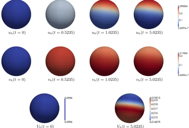
4.3.1. Instability for large cytosolic diffusion coefficient. First, we chooseD= 100. In Fig. 1 we see results in this case, showing contour plots of the solutions uh, vh, Vh evaluated on the level set Γh := {φh = 1/2} at different times. Thereby, one observes the evolution to an unstable stationary solution and towards an equilibrium with local maxima ofuh and vh on Γh. In a way this result shows similarities to Turing–type instabilities, where usually differences in diffusion constants drive the instability. In this case,d= 1 corresponds to equal lateral diffusion constants.
However, the large cytosolic diffusion admits the development of heterogeneities.
4.3.2. Stability for equal lateral and cytosolic diffusion coefficients. For D = d = 1, there is no instability as the results in Fig. 2 indicate.
4.3.3. Ellipsoidal membrane. We consider an ellipsoidal membrane Γ with semi-axes 0.75, 1 and 1.5. As in the first example we have used D = 100. In Fig. 3, the evolution towards a nearly stationary discrete solution uh on the level set {φh= 12} is displayed.
5. Numerical Treatment of the Non-local System
In this section, we use a parametric finite element description of the non-local system (3.1)–
(3.3) in order to numerically investigate instabilities for d= 1 found in Sec. 3. For this purpose, we apply the algorithm described in [17]. To discretize in time, we apply a semi-implicit Euler scheme, where all nonlinearities are linearized in a suitable way. We use a parametric finite element approach [2] with linear finite elements, where we solve as a system for the two concentrations u, von the membrane. The non-local term is treated fully explicitly. The resulting linear system is solved by a stabilized bi-conjugate gradient method (BiCGStab). The scheme is implemented using the adaptive finite element toolbox AMDiS [21].
uh(t= 0) uh(t= 0.5235) uh(t= 1.0235) uh(t= 5.0235)
vh(t= 0) vh(t= 0.5235) vh(t= 1.0235) vh(t= 5.0235)
Vh(t= 0) Vh(t= 5.0235)
Figure 1. Instability for increased cytosolic diffusion (D = 100). From left to right: the discrete solutionsuh (upper row),vh(middle row) on level set {φh= 12}fort= 0, t= 0.5235, t= 1.0235, andt= 5.0235, discrete solutionVhon level set{φh=12}fort= 0,t= 5.0235 (lower row).
uh(t= 0) uh(t= 5.0235) vh(t= 0) vh(t= 5.0235)
Vh(t= 0) Vh(t= 5.0235)
Figure 2. Stability for equal membrane and cytosolic diffusion coefficients (D= 1). From left to right: The discrete initial and stationary solutionsuh,vhandVhon level set{φh=12}.
5.1. Numerical Examples. In all following examples we use for f and q the specific choices proposed in (A.10) and (A.11), respectively. Thereby, we use parameters from Table 2. Fur- thermore, we consider the unit-sphere Γ = S2 and its discrete approximation Γh through a triangulation with a uniform grid. We assume random initial conditions u0 : Γh → [0,0.0002], v0 : Γh →[0,0.0002]. Moreover, we chooseVinit = 5.1. Note that this choice of initial conditions is the exact counterpart of the initial conditions used for the simulation of the full system in Section 4.
uh(t= 0) uh(t= 2.0235) uh(t= 12.0235) uh(t= 27.0235)
Figure 3. Instability for increased cytosolic diffusion (D = 100). From left to right: the discrete solutionsuhon level set{φh=12}fort= 0,t= 2.0235,t= 12.0235, andt= 27.0235.
parameter d γ a1 a2 a3 a4 a5 a6 a−6
value 1 400 0.02 20 160 1 0.5 0.36 5 Table 2. Parameters used for numerical results (non-local model).
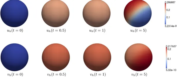
5.1.1. Instability with equal lateral diffusion coefficients. In Fig. 4, one can see contour plots of the discrete solutions uh, vh at different times ford= 1. Similarly to the first example in Sec. 4, one observes an evolution to an unstable spatially homogeneous solution and towards a stationary solution with a single spot pattern, which is in agreement with remarks in Sec. 3.
uh(t= 0) uh(t= 0.5) uh(t= 1) uh(t= 5)
vh(t= 0) vh(t= 0.5) vh(t= 1) vh(t= 5)
Figure 4. Instability with diffusion (d = 1). From left to right: the discrete solutions uh
(upper row),vh(lower row) fort= 0,t= 0.5,t= 1, andt= 5.
5.1.2. Stability for increased diffusion. For increased diffusion coefficient, the instability vanishes, see Fig. 5. Here we have scaled f, q and time t by a factor 1/10, which corresponds to scaling the diffusion coefficientsdu anddv in the dimensional formulation (see the appendix) by a factor 10. To be more precise, we have decreased the value of γ from 400 as in Table 2 to 40 and have rescaled time. The explanation for the stabilization by lowering the value of γ is that the inequality (2.47) is violated for small enoughγ. In an informal way one could explain this effect as a consequence of the ‘decreased difference’ between cytosolic diffusion constant D = ∞ and lateral membrane diffusionsdu, dv. This suggests, that fordu =dv and an Case 2 instability large differences betweenDanddu, dv are required, which resembles a classical Turing type mechanism in theV,uvariables.
5.1.3. Rich Nonlinear Dynamics. In Fig. 6, we present results showing the rich dynamics the model includes. Thereby we replace the corresponding parameters in Table 1 by the values
uh(t= 0) uh(t= 7) vh(t= 0) vh(t= 7)
Figure 5. Stability for increased diffusion: The discrete initial and stationary solutions uh
(left),vh(right).
given in Table 3. One observes that the system evolves to a homogeneous stationary which is unstable and later forms a pattern, which is again unstable. Finally the system reaches a stable homogenous stationary state, different from the initial one.
parameter d γ a1 a2 a3 a4 a5 a6 a−6 Vinit value 1 2000 0.001 20 160 1 0.5 0.36 10.3757 10.1
Table 3. Parameters used for numerical results in Fig. 6.
uh(t= 0) uh(t= 1.85) uh(t= 3.2) uh(t= 3.45)
Figure 6. Rich nonlinear dynamics for different set of parameters: discrete solution uh at initial time, att= 1.85 showing an unstable intermediate solution, att= 3.2 with an intermediate pattern and homogenous stationary solution.
6. Discussion
We have analytically and numerically studied a coupled system of surface–bulk reaction–
diffusion equations. Such a system for example arises in [17] as a model for the GTPase cycle in biological cells. Here the relevant quantities are the concentrationsu, v of active and inactive GTPase on the membrane, and the concentration V of inactive GTPase in the cytosolic vol- ume. Our main interest here was to analyze the possibility of a symmetry breaking. The latter refers to an instability of spatially homogeneous stationary points that are stable with respect to symmetry-conserving perturbations, which in our case means that u, v, and the boundary values of V are spatially homogeneous.
For spherical cell shapes we have performed a linearized stability analysis and have discovered that two different mechanisms for symmetry breaking are present. The first one requires a large difference in the lateral diffusion constants of u and v, expressed by a large value of din (1.1)–
(1.4). This mechanism is closely related to a classical Turing instability for a two-variable system withuas activator andv as substrate. The second mechanism however does even occur for equal lateral diffusion constants of u and v, i.e. even for d = 1, which is much more realistic in the application to the GTPase cycle in cells. This second mechanism on the other hand requires that the cytosolic diffusion coefficient D is much larger than the lateral diffusion coefficients.
The simulations show that a factor of 100 between both is sufficient, which is about the ratio between cytosolic and lateral membrane diffusion measured for biological cells [10]. The new