SFB 823
The U. S. fracking boom:
Impact on oil prices
Discussion Paper Manuel Frondel, Marco Horvath
Nr. 16/2018
The U. S. Fracking Boom:
Impact on Oil Prices
Manuel Frondel ∗ and Marco Horvath † July 30, 2018
As of late 2008, the steady decline of U. S. crude oil production over the last decades was reversed by the increased adoption of the hydraulic fracturing (“fracking”) technology. Adapting the supply-side model pro- posed by Kaufmann et al. (2004) to assess OPEC’s ability to influence real oil prices, this paper investigates the effect of the increase in U. S. oil pro- duction due to fracking on world oil prices. Among our key results ob- tained from (dynamic) OLS estimations, there is a statistically significant negative long-run relationship between increased U. S. oil production and oil prices.
Keywords: Dynamic OLS, Error Correction Model, Shale Oil.
JEL codes: Q41, Q32, L71.
Acknowledgements: We are grateful for invaluable comments and suggestions by Aisling Reynolds-Feighan, Colin Vance and four anonymous reviewers. This paper also benefitted from discussions with the audiences at the 9th RGS Doctoral Con- ference in Economics in Bochum (Germany), the 4th PhD Workshop in Economics in Braga (Portugal), the 7th Atlantic Workshop on Energy and Environmental Eco- nomics in A Toxa (Spain) and the 21st Workshop of the GEE Student Chapter in Aachen (Germany). Marco Horvath gratefully acknowledges financial support by the
∗RWI Leibniz Institute for Economic Research, Ruhr Graduate School in Economics, and Ruhr University Bochum
†RWI Leibniz Institute for Economic Research, Ruhr Graduate School in Economics, and Ruhr University Bochum, correspondence to: Manuel Frondel, RWI, Hohenzollernstr. 1-3, 45128 Essen, Germany. E-Mail:frondel@rwi-essen.de
Ruhr Graduate School in Economics, the Commerzbank Foundation, and the Fritz
Thyssen Foundation. This work has also been supported by the Collaborative Re-
search Center “Statistical Modeling of Nonlinear Dynamic Processes” (SFB 823) of
the German Research Foundation (DFG), within Project A3, “Dynamic Technology
Modeling”.
1 Introduction
Since the outset of the new millennium, the global oil market has experienced signif- icant changes: Due to the surge of petroleum consumption from emerging countries, world crude oil demand has substantially increased, not least driven by China (Smith, 2009). In fact, global oil demand increased by more than 25% between 2000 and 2017, from about 76.9 to 98.2 million barrels per day (mbd), with China accounting for more than 8 mbd of this increase (BP, 2018). On the supply side, while about one third of crude oil production still originates from the member countries of the Orga- nization of the Petroleum Exporting Countries (OPEC), the production of Non-OPEC countries strongly increased in the last decade, most notably as a consequence of hy- draulic fracturing, also known as “fracking”. In conjunction with horizontal drilling and micro-seismic imaging, the use of this set of technologies, which was originally developed for the exploration of natural gas, allows for tapping into oil reservoirs that are trapped in shale siltstone and clay stone formations (Maugeri, 2012). Oil ex- tracted on the basis of fracking techniques is commonly referred to as tight or shale oil to differentiate it from crude oil obtained by conventional drilling methods.
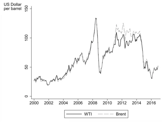
To date, the commercial use of this set of technologies, usually subsumed by the notion of fracking, has been limited to the U. S. (Kilian, 2017b), where the steady decline of crude oil production as of the 1970s was reversed by adopting this technol- ogy. Owing to fracking, U. S. crude oil production almost doubled over the past 15 years (see Figure 1). Thus, the advance of fracking was often called a game changer for the global oil market. Its importance may even further increase given that numer- ous other Non-OPEC countries contemplate intensifying the usage of this technology.
Notably, in addition to Australia, India, and several European countries, such as the
UK, Russia, one of the world’s largest oil producers, has commenced investigating
the potentials of fracking (EIA, 2013). As a result, it is frequently announced in the
press that OPEC’s market power has drastically diminished.
Figure 1: Shale Oil and Total Crude Oil Production in the U. S. (left-hand scale) and Share of Shale Oil in Total U. S. Crude Oil Production (right-hand scale).
0%10%20%30%40%50%60%
0246810
million barrels per day
2000 2002 2004 2006 2008 2010 2012 2014 2016 US shale oil production
US conventional crude oil production Share of shale oil
Using monthly data on the U. S. oil market spanning from January 2000 to Decem- ber 2016 and taking the demand side as given, this paper modifies the supply-side model developed by Kaufmann et al. (2004) to explore the effect of fracking on world oil prices. To gauge the short-run effects, we employ a two-step Error Correction Model (ECM), while the long-run relationship between the crude oil price and frack- ing, as well as various OPEC supply factors, is estimated via standard and dynamic OLS methods. The key finding of our correlation analysis is a statistically significant negative long-run relationship between increased U. S. oil production due to frack- ing and world oil prices. A similarly negative influence is found for OPEC supply volumes that exceed the stipulated OPEC quota, indicating that OPEC still matters.
Although there is a vast oil market literature, fracking only recently has become
a topic of interest, and the economic impact of the emerging fracking oil supply is
not widely analyzed yet. Three notable exceptions are the review article by Kilian (2017a), the empirical study of Kilian (2017b), and the oil price forecasts of Baumeister and Kilian (2016) on the basis of a vector autoregressive (VAR) model. Kilian (2017a) provides an overview of the impact of fracking on U. S. oil and gasoline prices, ar- guing that the effect of increased U. S. shale oil production on the crude oil price is likely to have been near $10 per barrel.
Using a novel econometric technique, this estimate is confirmed by Kilian (2017b), who also estimates the cumulative losses of Saudi Arabian oil producers due to frack- ing at over 100 Billion US Dollars. Highlighting the role of economic activity for oil prices, Baumeister and Kilian (2016) provide quantitative evidence that a slowing global economy, rather than supply shocks, was the dominant reason for the $49 cumulative decline in the Brent price per barrel between June and December 2014.
These authors find that “$24 of the cumulative decline is unambiguously explained by a weakening of the global economy, which resulted in lower demand for crude oil” (Kilian, 2017a:198). Our study complements this strand of the literature by quan- tifying the impact of the advance of shale oil on the oil price using standard and dynamic OLS methods and (Vector) Error Correction Models, the results of which are employed to simulate the development of global oil prices in absence of the shale oil boom.
In contrast, former studies predominantly focussed on OPEC behavior. For in-
stance, the articles by Kaufmann (1995), Kaufmann et al. (2004), and Dees et al. (2007)
all investigate OPEC’s influence on oil prices over the medium- and long-run. These
authors find the two most important decision variables to be the OPEC production
quota, as well as the rate at which OPEC adds production capacity, which would sig-
nal tightness in the market. Dees et al. (2007) additionally point out that a breakdown
in the cooperation of the OPEC cartel results in a sharp drop in the crude oil price, as
competition among OPEC countries leads to supply quantities that surpass demand and go into stocks.
The following section provides a concise summary of the rise in U. S. oil produc- tion owing to fracking and OPEC’s behavioral reaction to the increased use of this technology. Section 3 explains the methods applied, followed by the presentation of our estimation results in Section 4. The last section summarizes and concludes.
2 U. S. Crude Oil Production and OPEC Behavior
Currently, the only country that permits fracking on a large scale is the U. S. , whereas many other countries are highly reluctant to employing this technology because of its potentially negative implications for the environment, notably potential hazards due to water pollution and seismic tremors – see the review article by Jackson et al. (2014) for a discussion of these environmental and health issues. France and Germany, for instance, have implemented a ban because of perceived health risks due to fracking.
In contrast, other countries, such as the UK and Australia, have recently modified political regulations to allow for fracking (EIA, 2013).
With the beginning of the surge in shale oil production in late 2008 (Kilian, 2017b), U. S. crude oil production steadily increased until the end of 2014, with the share of shale oil in total U. S. production rising from about 6% in January 2000 to almost 50% by the end of 2014 (see Figure 1). In fact, November 2008 marks the reversal in the long-standing decline in U. S. oil production, a reversal that is largely due to the U. S. fracking boom (Kilian, 2017b).
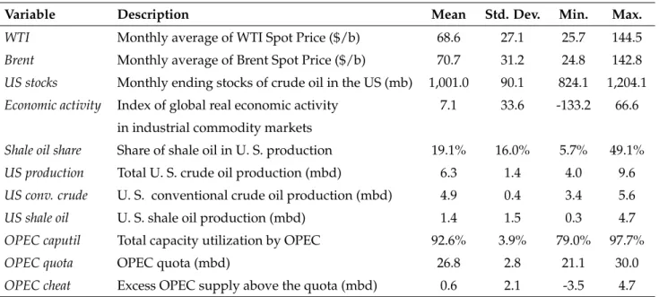
This boom exerted substantial pressure on the price of the light crude oil West Texas
Intermediate (WTI), whose price is the key indicator for U. S. crude oil, with the result
that the prices of WTI and Brent, the benchmark for European crude oil, drifted apart
between 2010 and 2015 (Figure 2). Prior to 2010, both price indicators had more or less
the same level, whereas afterwards WTI was significantly cheaper than Brent oil until the end of 2015, with differences in prices sometimes amounting to $10 per barrel or even more.
Recent studies suggest that this difference was the result of the increased shale oil supply, paired with a bottleneck in refinery and oil transport infrastructure (Boren- stein and Kellogg, 2014; Kilian, 2016). This price differential between WTI and Brent initially reflected the excess supply of light crude oil in Cushing, Oklahoma, where the WTI price is measured. Owing to the lack of pipelines to the refineries, this oil was stored in a location where it could not compete with imports (Kilian, 2016:193).
At the end of 2015, the price differential virtually vanished due to the expansion of transport infrastructure. It allowed light crude oil that used to be landlocked in the center of the U. S. to reach existing refineries.
Figure 2: Crude Oil Prices on West Texas Intermediate (WTI) and Brent Oil
050100150
US Dollar per barrel
2000 2002 2004 2006 2008 2010 2012 2014 2016
WTI Brent
While world oil prices shrank by $49 between June and December 2014, under the
lead of Saudi-Arabia, OPEC changed its strategy from defending oil prices to defend- ing market shares and refrained from its former behavior of curbing oil production to attempt to stabilize world oil prices. Prior to this change, the OPEC members usually agreed upon individual production allocations for each country and, hence, an upper limit for the total OPEC production level, the OPEC quota, thereby assuming that OPEC can maximize its profits when the production quota is optimally set (Griffin, 1985).
Employing the quota as a key instrument, it is the declared aim of the OPEC cartel
”to coordinate and unify the petroleum policies of its Member Countries and ensure the stabilization of oil markets in order to secure an efficient, economic and regular supply of petroleum to consumers, a steady income to producers and a fair return on capital for those investing in the petroleum industry” (OPEC, 2018). There is evi- dence, though, that OPEC is not operating as a perfect cartel: By comparing various potential market structures that could explain OPEC behavior, Smith (2005) points out that the OPEC members operate much more like a non-cooperative oligopoly than a frictionless cartel. Moreover, while according to Kaufmann et al. (2008) OPEC uses its market power by appointing quotas, thereby influencing both oil production and prices, these authors also find that OPEC behavior has some competitive ele- ments, as for example higher oil prices lead to increasing production of individual OPEC countries.
The OPEC quota was regularly varied and posted on the organization’s home-
page until November 2007, but was updated only irregularly thereafter. For instance,
with an OPEC crude oil production of 24.85 million barrels per day (mbd), the of-
ficial quota of January 2009 remained in place until November 2011, when OPEC
announced an increase in the quota to 30 mbd. Frequently, however, the actual OPEC
production level substantially exceeded the announced quota, a behavior that is cap-
tured here by the variable OPEC cheat (for its definition, see Table 1). In December 2016, for example, the OPEC production exceeded the quota by about 3 mbd.
Table 1: Summary Statistics for the Variables employed in the Empirical Analysis
Variable Description Mean Std. Dev. Min. Max.
WTI Monthly average of WTI Spot Price ($/b) 68.6 27.1 25.7 144.5
Brent Monthly average of Brent Spot Price ($/b) 70.7 31.2 24.8 142.8 US stocks Monthly ending stocks of crude oil in the US (mb) 1,001.0 90.1 824.1 1,204.1 Economic activity Index of global real economic activity 7.1 33.6 -133.2 66.6
in industrial commodity markets
Shale oil share Share of shale oil in U. S. production 19.1% 16.0% 5.7% 49.1%
US production Total U. S. crude oil production (mbd) 6.3 1.4 4.0 9.6 US conv. crude U. S. conventional crude oil production (mbd) 4.9 0.4 3.4 5.6
US shale oil U. S. shale oil production (mbd) 1.4 1.5 0.3 4.7
OPEC caputil Total capacity utilization by OPEC 92.6% 3.9% 79.0% 97.7%
OPEC quota OPEC quota (mbd) 26.8 2.8 21.1 30.0
OPEC cheat Excess OPEC supply above the quota (mbd) 0.6 2.1 -3.5 4.7
Note: Number of observations for all variables: 204. Data sources: EIA (2018), OPEC (2007), OPEC press releases, and Kilian (2009).
At its November meeting in 2016, OPEC changed its strategy again and, in a broad alliance with Non-OPEC oil producing countries, most notably the world’s largest oil producer Russia, decided to cut global production by 1.8 mbd to push world oil prices. This cut in production was officially reconfirmed in January 2017, when OPEC (2016) announced the new quota of 32.5 mbd.
Presumably due to the recovery of global oil prices in the aftermath of the OPEC
decision at the end of 2016, but probably also encouraged by OPEC’s announcements
with respect to production cuts, U. S. oil production from fracking has been revital-
ized, which will likely put downward pressure on oil prices. Using standard and
dynamic OLS methods and (Vector) Error Correction Models, in what follows, we
investigate whether fracking indeed negatively affects oil prices. For this analysis,
we primarily draw on monthly data from the US Energy Information Administration
(EIA, 2018), which reports price information, US supply factors, as well as OPEC ca-
pacity and production. Information on the OPEC quota can be gathered from the 2007 OPEC Annual Statistical Bulletin (OPEC, 2007) and from several OPEC press releases for the years after 2007. Summary statistics for the whole period from January 2000 until December 2016, covering 204 months, are reported in Table 1, annual averages are displayed in Table A3 in the appendix. For replication purposes, the database is available from the authors upon request.
3 Methodology
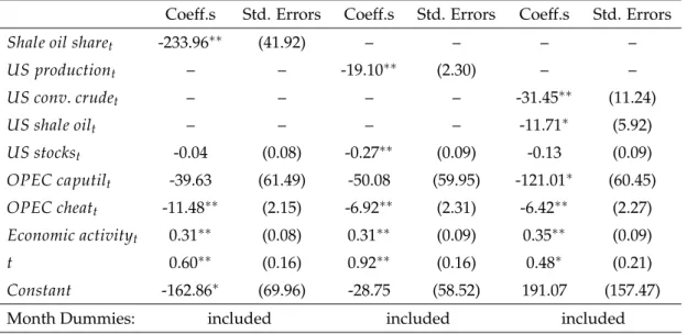
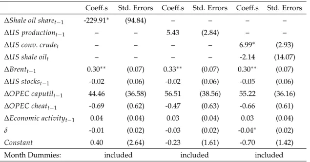
Our analysis focuses on WTI and the U. S. oil market, as the U. S. is both the world’s largest consumer of crude oil and the largest producer of shale oil. Given the close coincidence of WTI and Brent prices in most years (Figure 2), the empirical results are very similar when Brent, rather than WTI prices are employed for estimating the model specifications presented below (see Tables A4 to A7 in the Appendix).
To explore the long-term impacts of fracking on inflation-adjusted monthly average WTI spot prices, we estimate a modified specification of the pricing rule developed by Kaufmann et al. (2004):
WT I
t= α
0+ α
1Fracking
t+ α
2US stocks
t+ α
3OPEC caputil
t+
α
4OPEC cheat
t+ α
5Economic activity
t+ α
tt + αM
t+ µ
t,
(1)
where µ denotes an idiosyncratic error term and Fracking stands for two alterna-
tive variables, either total U. S. crude oil production or the share of shale oil in total
U. S. production, the latter being the basis for a simulation exercise presented in the
results section. Also in contrast to Kaufmann et al. (2004), we have added a time trend
t to capture the secular trend of increasing world oil demand and, hence, potential re-
source scarcities, as well as a variable to reflect potential impacts of U. S. crude oil
stocks (for average volumes, see Table 1 and Table A3), and a vector M of 11 month dummies to account for the seasonality of the data, with the December dummy being omitted.
In line with Kaufmann et al. (2004), we have also included variables that reflect the influence of OPEC: a measure capturing OPEC’s total capacity utilization (OPEC caputil), calculated by dividing total OPEC production by total OPEC capacity, and a variable representing the excess supply by OPEC above the quota, called OPEC cheat.
In contrast to Kaufmann et al. (2004), we have refrained from including the OPEC quota in equation (1), as this quota was not regularly updated in recent years and, thus, its variation is quite low (see Table 1 for the low standard deviation relative to that of the variable OPEC cheat). Moreover, the quota is highly correlated with the variable OPEC cheat, rendering the inclusion of the OPEC quota redundant. Fi- nally, in contrast to Kaufmann et al. (2004), we have included an index of global real economic activity in industrial commodity markets (Economic activity). This index was developed by Kilian (2009) to capture economic up- and downturns, which are likely to affect global oil prices.
1Further differences to the specification of Kaufmann et al. (2004) are the usage of monthly, rather than quarterly data and the inclusion of U. S. crude oil stocks instead of days of forward consumption, for which monthly data is lacking.
In an alternative specification, instead of either including total U. S. crude oil pro- duction or the share of shale oil in total U. S. production, we distinguish between the U. S. conventional crude and shale oil production, as given by the variables US conv. crude and US shale oil, respectively, to reflect the take-off of the US shale
1Data on this index can be downloaded from Professor Kilian’s homepage: http://
www-personal.umich.edu/~lkilian/.
oil production:
WT I
t= β
0+ β
1US conv. crude
t+ β
2US shale oil
t+ β
3US stocks
t+ β
4OPEC caputil
t+ β
5OPEC cheat
t+ (2) + β
6Economic activity
t+ β
tt + βM
t+ µ
t.
Long-run effects are estimated on the basis of equations (1) and (2) using both stan- dard and dynamic OLS methods. Yet, OLS methods may yield biased estimates, as as- sumptions on autocorrelation and homoscedasticity may be violated. Dynamic OLS (DOLS) methods, first developed by Stock and Watson (1993), cope with these vi- olations: to account for the dynamic effects and autocorrelations within time series data, in addition to the regressors in levels, n leads and n lags of the regressors in first differences are included in the estimation specification. The DOLS estimator is consis- tent, asymptotically normally distributed, and efficient (Stock and Watson, 1993). The number of leads and lags is typically determined on the basis of information criteria such as the Akaike (AIC) and Bayesian Information Criterion (BIC). If heteroskedas- ticity is an issue, Zivot and Wang (2007) suggest estimating Newey-West Standard Errors to obtain consistent estimates, a suggestion that we followed in our OLS and DOLS estimations.
To examine the short-term relationship among the variables included in equations
(1) and (2), we estimate Error Correction Models (ECM), using the two-step tech-
nique proposed by Engle and Granger (1987). In the first step, the residuals µ of the
long-term relationships (1) and (2) are estimated using DOLS methods. In the second
step, the first difference of the dependent variable ∆WT I
t: = WT I
t− WT I
t−1is re-
gressed upon the lagged residuals µ
t−1and the first differences of the regressors, as
the optimal number of lags, indicated by both AIC and BIC, is one. For the long-term
relationship (1), the corresponding ECM reads:
∆WT I
t= γ
0+ δµ
t−1+ γ
1∆Fracking
t−1+ γ
2∆US stocks
t−1+ γ
3∆OPEC caputil
t−1+ γ
4∆OPEC cheat
t−1(3) + γ
5∆Economic activity
t−1+ γM
t+ e
t,
where δ reflects the rate of adjustment to equilibrium after a shock in the market. As the residuals capture the difference between the actual value of the crude oil price and the long-run prediction of pricing equation (1), statistical significance of δ indicates that the oil price deviates from its long-term equilibrium. In a similar vein, the ECM corresponding to the long-term relationship (2) reads:
∆WT I
t= ρ
0+ δµ
t−1+ ρ
1∆US conv. crude
t−1+ ρ
2∆US shale oil
t−1+ ρ
3∆US stocks
t−1+ ρ
4∆OPEC caputil
t−1+ ρ
5∆OPEC cheat
t−1(4) + ρ
6∆Economic activity
t−1+ ρM
t+ e
t.
As a robustness check, in addition to estimating short-run relationships on the basis of an ECM, we use a Vector Error Correction Model (VECM), as it has the advantage that short- and long-run relationships can be estimated simultaneously. The short-run effects are given by the coefficient estimates of the regressors in first differences, while the long-run relationship is reflected by the cointegrating vector, whose components are denoted by θ
1and θ
2, while δ again represents the adjustment rate to equilibrium.
Following Kaufmann et al. (2004), the VECM is estimated using all the right-hand
side variables of specifications (1) and (2), respectively, which are gathered in vector
x:
∆WT I
t= δ ( θ
1WT I
t−1+ θ
2x
t−1) +
∑
n i=1( λ
i∆WT I
t−i+ φ
i∆ x
t−i) + θM
t+ µ
t, (5)
with λ
i, φ
i, and θ
1being coefficients to be estimated and θ
2and θ denoting coefficient vectors.
4 Estimation Results
To test for the stationarity of the variables included in pricing equations (1) and (2), augmented Dickey-Fuller (ADF) tests are employed. As the null hypothesis of a unit root is not rejected throughout (see Table A1 in the Appendix) and ADF tests reject the null hypothesis of a unit root in the first differences of these variables, we conclude that all variables are integrated of order one: I(1). Furthermore, again using ADF tests to examine whether the residuals of the long-run relationship (1) and (2) are stationary (Engle and Granger, 1987) suggests that the variables included in both equations are cointegrated (see Table A2 in the Appendix).
Comparing the OLS and DOLS coefficient estimates of the long-run relationships
(1) and (2) reported in Tables 2 and 3, we find that signs and significance levels are
largely similar across specifications and estimation techniques. Consistent with eco-
nomic theory (Dees et al., 2007), both U. S. production and U. S. stocks have a signif-
icantly negative effect on the crude oil price: higher production levels and increases
in stocks put downward pressure on the price, as reliance on current production is
diminished, thereby reducing the risk premium associated with a supply disruption
(Kaufmann et al., 2004:77). Notably, the share of shale oil in total U. S. production
also negatively impacts oil prices. This does not come as a surprise: Given a fairly
stable conventional crude oil production, increasing shares of shale oil are associated
with increases in total U. S. production.
Table 2: OLS Estimation Results for Pricing Rules (1) and (2) for WTI
Pricing Rule (1) Pricing Rule (2)
Coeff.s Std. Errors Coeff.s Std. Errors Coeff.s Std. Errors
Shale oil sharet -269.16∗∗ (61.67) – – – –
US productiont – – -17.79∗∗ (2.07) – –
US conv.crudet – – – – -21.07∗ (9.45)
US shale oilt – – – – -16.34∗∗ (4.81)
US stockst -0.42∗∗ (0.07) -0.31∗∗ (0.05) -0.31∗∗ (0.05)
OPEC caputilt 67.57 (63.54) 10.43 (39.41) 0.23 (53.37)
OPEC cheatt -3.65∗ (1.64) -4.00∗∗ (1.22) -3.88∗∗ (1.26) Economic activityt 0.20∗ (0.09) 0.26∗∗ (0.05) 0.27∗∗ (0.06)
t 1.40∗∗ (0.19) 0.91∗∗ (0.08) 0.87∗∗ (0.16)
Constant -351.22∗∗ (84.83) -61.96∗ (30.34) -16.82 (138.70)
Month Dummies: included included included
Note:∗denotes significance at the 5%-level and∗∗at the 1%-level, respectively. Newey-West Standard Errors are in parentheses.
Table 3: Dynamic OLS Estimation Results for Pricing Rules (1) and (2) for WTI
Pricing Rule (1) Pricing Rule (2)
Coeff.s Std. Errors Coeff.s Std. Errors Coeff.s Std. Errors
Shale oil sharet -193.66∗∗ (37.31) – – – –
US productiont – – -15.14∗∗ (1.89) – –
US conv.crudet – – – – -26.47∗ (10.88)
US shale oilt – – – – -9.58 (5.17)
US stockst 0.07 (0.07) -0.12 (0.07) -0.05 (0.07)
OPEC caputilt -136.85∗∗ (52.10) -118.99∗∗ (42.09) -163.18∗∗ (50.87) OPEC cheatt -12.59∗∗ (1.84) -8.53∗∗ (1.71) -7.87∗∗ (1.71) Economic activityt 0.50∗∗ (0.07) 0.48∗∗ (0.07) 0.50∗∗ (0.07)
t 0.34∗ (0.15) 0.59∗∗ (0.12) 0.30 (0.19)
Constant -46.52 (58.86) 50.90 (41.34) 224.93 (149.86)
Month Dummies: included included included
Note:∗denotes significance at the 5%-level and∗∗at the 1%-level, respectively. Newey-West Standard Errors are in parentheses.
The coefficient estimates related to the considered OPEC supply factors are also in
line with theory (Kaufmann et al., 2004). First, the coefficient estimate on OPEC cheat is negative across all specifications. This is a plausible result: If OPEC production exceeds the stipulated quota, this should put downward pressure on the oil price.
Second, in a similar vein, we interpret the negative sign of the coefficient estimate on OPEC capacity utilization in the DOLS estimation (Table 3): when a lot of crude oil is refined and placed on the market, this puts pressure on oil prices. Third, not surprisingly, the coefficient estimate of the indicator of economic activity is positive in all long-run specifications, indicating that a strong world-wide economic activity is associated with a higher world oil price.
Turning to the ECM results, we fail to see any kind of short-term relationship be- tween most of the supply factors and WTI prices (Table 4). Apart from µ
t−1, which has the expected negative sign reflecting the speed of adjustment to the long-run equilib- rium, the only coefficient estimate that is different from zero at conventional signifi- cance levels is that on the lagged first difference of the shale oil share (see first column of Table 4). Apparently, any increase in the share of shale oil in total U. S. crude oil production is associated with a decrease in the WTI price in the following period, a result that seems to be plausible given that the shale oil supply is more variable than conventional crude oil supply. This outcome is further supported by the estimates of the third specification, which reveal a negative relationship between shale oil produc- tion and the WTI price, but not between conventional crude oil and the WTI price.
The remaining estimation results may be explained by the fact that all the other
supply factors are quite stable in the short-term. This holds particularly true for the
OPEC quota, which is typically changed once a year, if at all. While the other OPEC
factors are not as stable as the OPEC quota, their monthly fluctuations are quite mod-
erate. It is thus not surprising that the majority of supply factors considered exhibit
vanishing short-term impacts. Finally, in qualitative terms, the ECM results reported
Table 4: Estimation Results for the Error Correction Models
ECM (3) ECM (4)
Coeff.s Std. Errors Coeff.s Std. Errors Coeff.s Std. Errors
∆Shale oil sharet−1 -269.88∗ (119.59) – – – –
∆US productiont−1 – – 4.26 (4.07) – –
∆US conv.crudet−1 – – – – 7.05 (4.06)
∆US shale oilt−1 – – – – -21.89∗ (10.91)
∆USstockst−1 -0.11 (0.06) -0.10 (0.06) -0.11∗ (0.06)
∆OPEC caputilt−1 35.44 (39.13) 30.64 (38.84) 40.95 (39.16)
∆OPEC cheatt−1 -1.06 (0.57) -0.97 (0.60) -0.94 (0.58)
∆Economic activityt−1 0.04 (0.04) 0.05 (0.04) 0.04 (0.03)
µt−1 -0.26∗∗ (0.08) -0.23∗∗ (0.07) -0.24∗∗ (0.06)
Constant -2.44 (1.69) -3.21 (1.73) -2.74 (1.65)
Month Dummies: included included included
Note:∗denotes significance at the 5%-level and∗∗at the 1%-level, respectively.
in Table 4 are mimicked by the estimates obtained from applying the VECM (5), which are reported in Table 5.
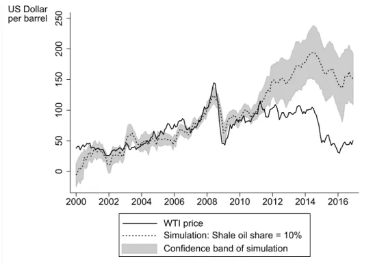
To get a sense of the magnitude of the effect of shale oil production on the oil price, we now present the results of a simulation exercise based on the long-run estimation results of equation 1. Holding the shale oil share constant at 10%, that is, the share before the fracking boom started in 2008 (Figure 1), this simulation exercise predicts the WTI price using the actual values of the U. S. and OPEC supply factors, as well as the indicator of economic activity. According to this prediction, oil prices would have been around 40 to 50 dollars per barrel higher if the shale oil share had remained constant at 10%, that is, if there had not been a fracking boom in the U. S. (Figure 3).
The effect resulting from this simulation is quite high compared to the estimate of 10
dollars per barrel provided by Kilian (2017b), which among other things is due to the
fact that in our specifications the demand side is taken as given.
Table 5: Estimation Results for the Vector Error Correction Models
Pricing Rule (1) Pricing Rule (2) Coeff.s Std. Errors Coeff.s Std. Errors Coeff.s Std. Errors
∆Shale oil sharet−1 -203.13∗ (89.35) – – – –
∆US productiont−1 – – 5.96∗ (2.72) – –
∆US conv.crudet−1 – – – – 6.53∗ (2.83)
∆US shale oilt−1 – – – – 5.06 (12.52)
∆WT It−1 0.31∗∗ (0.07) 0.35∗∗ (0.07) 0.31∗∗ (0.07)
∆USstockst−1 -0.06 (0.05) -0.06 (0.05) -0.09 (0.05)
∆OPEC caputilt−1 35.29 (35.74) 46.65 (37.27) 49.33 (35.15)
∆OPEC cheatt−1 -0.55 (0.60) -0.34 (0.60) -0.47 (0.59)
∆Economic activityt−1 0.03 (0.04) 0.02 (0.04) 0.02 (0.04)
δ -0.02 (0.02) -0.04∗ (0.02) -0.06∗∗ (0.02)
Constant -0.26 (1.69) -0.88 (1.49) -0.92 (1.38)
Month Dummies: included included included
Note:∗denotes significance at the 5%-level,∗∗at the 1%-level, respectively.
Figure 3: Simulation holding the Shale Oil Share Constant at the Pre-Fracking-Boom Value of 10%
050100150200250
US Dollar per barrel
2000 2002 2004 2006 2008 2010 2012 2014 2016
Confidence band of simulation WTI price
Simulation: Shale oil share = 10%
5 Summary and Conclusion
The steady decline in U. S. crude oil production over the last decades was reversed by the increased adoption of the technology of hydraulic fracturing, also known as
“fracking”. This technology is often called a game changer for the global oil market, as it enabled the U. S. to become one of the world’s largest crude oil producers again.
In this vein, it has been frequently announced in the press that OPEC’s market power, if still existing at all, has drastically diminished.
Using monthly data spanning from January 2000 to December 2016 and a supply- side model similar to that proposed by Kaufmann et al. (2004), this study has investi- gated the effect of fracking on the world crude oil price. Among the key results of our correlation analysis is the finding of a statistically significant negative long-run rela- tionship between the oil price and OPEC supply volumes that exceed the announced OPEC quota, indicating that OPEC still matters. We also find a negative influence of the increased U. S. oil production due to fracking on the oil price, a result that is in line with the studies of Borenstein and Kellogg (2014) and Kilian (2017b). Further- more, a simulation exercise demonstrates that oil prices would have been around 40 to 50 dollars per barrel higher if the U. S. fracking boom had not occurred, an effect that is quite high due to the fact that in our specifications the demand side is taken as given. This exercise indicates that it is important to model both the supply and demand side to not overestimate the impact of a single factor, such as the additional oil supply due to fracking.
Nonetheless, while being non-causal in nature, this empirical evidence substanti-
ates the conclusion of Kilian (2017b) that without a doubt, the U. S. fracking boom
is an example of a technological change in a single industry of one country affecting
international trade worldwide, not least world oil prices. Moreover, as it is likely
that the fracking technology is also used more intensively in countries other than the
U. S. , it can be expected that the pressure that this technology exerts on world oil
prices may further increase. However, fracking is just one of a multitude of factors
that influence oil prices, among which the global economic development is the most
important. Therefore, given the empirical evidence that oil supply shocks tend to
have only modest effects on the price of oil (Kilian, 2016), one should not expect a
further drastic decrease in oil prices due to fracking.
6 Appendix
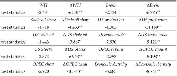
Table A1: Augmented Dickey-Fuller (ADF) Test Results
WTI ∆WTI Brent ∆Brent
test statistics -2.481 -6.581∗∗ -2.134 -6.775∗∗
Shale oil share ∆Shale oil share US production ∆US production
test statistics -1.718 -4.263∗∗ -1.303 -11.189∗∗
US shale oil ∆US shale oil US conv. crude ∆US conv. crude
test statistics -1.443 -3.867∗ -2.930 -9.121∗∗
US Stocks ∆US Stocks OPEC caputil ∆OPEC caputil
test statistics -2.373 -6.943∗∗ -2.753 -8.193∗∗
OPEC cheat ∆OPEC cheat Economic Activity ∆Economic Activity
test statistics -2.920 -10.843∗∗ -3.085 -8.741∗∗
Note:∗denotes significance at the 5%-level,∗∗at the 1%-level, respectively. ADF tests include an intercept and a time trend. The number of lags is selected using the Akaike information criterion. Test statistics are taken from MacKinnon (1996) using the number of observations.
Table A2: Cointegration Tests based on Augmented Dickey-Fuller (ADF) Tests on the Residuals of Equations (1) and (2)
Pricing Rule (1) Pricing Rule (2) Shale oil share US production US shale oil & US conv. crude test statistics (without trend and constant) -4.057∗∗ -5.397∗∗ -5.520∗∗
test statistics (with time trend) -4.239∗∗ -5.388∗∗ -5.509∗∗
Note:∗denotes significance at the 5%-level,∗∗at the 1%-level, respectively. The number of lags is selected using the Akaike information criterion. Test statistics are taken from MacKinnon (1996) using the number of observations.
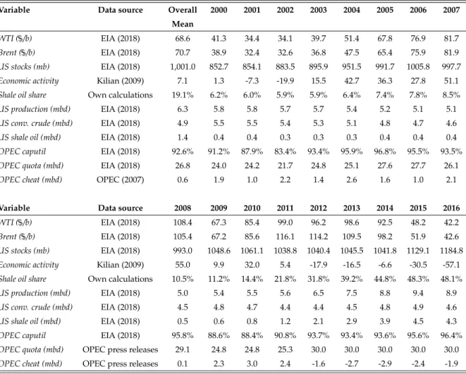
Table A3: Overall and Yearly Averages in terms of Means
Variable Data source Overall 2000 2001 2002 2003 2004 2005 2006 2007
Mean
WTI ($/b) EIA (2018) 68.6 41.3 34.4 34.1 39.7 51.4 67.8 76.9 81.7
Brent ($/b) EIA (2018) 70.7 38.9 32.4 32.6 36.8 47.5 65.4 75.9 81.9
US stocks (mb) EIA (2018) 1,001.0 852.7 854.1 883.5 895.9 951.5 991.7 1005.8 997.7
Economic activity Kilian (2009) 7.1 1.3 -7.3 -19.9 15.5 42.7 36.3 27.8 51.1
Shale oil share Own calculations 19.1% 6.2% 6.0% 5.9% 5.9% 6.4% 7.4% 7.8% 8.5%
US production (mbd) EIA (2018) 6.3 5.8 5.8 5.7 5.7 5.4 5.2 5.1 5.1
US conv. crude (mbd) EIA (2018) 4.9 5.5 5.5 5.4 5.3 5.1 4.8 4.7 4.6
US shale oil (mbd) EIA (2018) 1.4 0.4 0.4 0.3 0.3 0.3 0.4 0.4 0.4
OPEC caputil EIA (2018) 92.6% 91.2% 87.9% 83.4% 93.4% 95.9% 96.8% 95.5% 93.5%
OPEC quota (mbd) EIA (2018) 26.8 24.0 24.2 21.7 24.8 25.1 27.6 27.7 26.1
OPEC cheat (mbd) OPEC (2007) 0.6 1.9 1.0 2.2 1.4 2.6 1.6 1.0 2.1
Variable Data source 2008 2009 2010 2011 2012 2013 2014 2015 2016
WTI ($/b) EIA (2018) 108.4 67.3 85.4 99.0 96.2 98.6 92.5 48.2 42.2
Brent ($/b) EIA (2018) 105.4 67.2 85.6 116.1 114.2 109.5 98.2 51.9 42.6
US stocks (mb) EIA (2018) 993.0 1048.6 1061.1 1038.8 1040.4 1045.5 1041.8 1129.1 1184.8
Economic activity Kilian (2009) 55.0 9.9 32.0 5.4 -17.9 -16.5 -6.6 -30.5 -57.1
Shale oil share Own calculations 10.5% 11.2% 14.4% 21.8% 31.8% 39.2% 44.8% 48.3% 48.1%
US production (mbd) EIA (2018) 5.0 5.4 5.5 5.6 6.5 7.5 8.8 9.4 8.9
US conv. crude (mbd) EIA (2018) 4.5 4.8 4.7 4.4 4.4 4.5 4.8 4.9 4.6
US shale oil (mbd) EIA (2018) 0.5 0.6 0.8 1.2 2.1 2.9 3.9 4.5 4.3
OPEC caputil EIA (2018) 95.8% 88.6% 88.4% 90.8% 93.7% 93.4% 93.6% 95.6% 96.4%
OPEC quota (mbd) OPEC press releases 29.1 24.8 24.8 25.3 30.0 30.0 30.0 30.0 30.0
OPEC cheat (mbd) OPEC press releases 0.1 2.3 3.0 2.4 -1.6 -2.7 -2.9 -2.4 -1.9
Table A4: OLS Estimation Results for Pricing Rules (1) and (2) for Brent Oil
Coeff.s Std. Errors Coeff.s Std. Errors Coeff.s Std. Errors
Shale oil sharet -304.76∗∗ (71.78) – – – –
US productiont – – -21.50∗∗ (2.50) – –
US conv.crudet – – – – -24.65∗ (12.10)
US shale oilt – – – – -20.11∗∗ (5.77)
US stockst -0.54∗∗ (0.10) -0.42∗∗ (0.06) -0.42∗∗ (0.06) OPEC caputilt 85.83 (79.10) 24.16 (48.19) 14.38 (67.61)
OPEC cheatt -2.84 (2.05) -3.56∗ (1.50) -3.44∗ (1.50)
Economic activityt 0.11 (0.12) 0.16∗ (0.06) 0.17∗ (0.08)
t 1.73∗∗ (0.24) 1.19∗∗ (0.10) 1.15∗∗ (0.19)
Constant -424.24∗∗ (103.39) -95.84∗ (37.63) -52.55 (175.94)
Month Dummies: included included included
Note:∗denotes significance at the 5%-level and∗∗at the 1%-level, respectively. Newey-West Standard Errors are in parentheses.
Table A5: Dynamic OLS Estimation Results for Pricing Rules (1) and (2) for Brent Oil Coeff.s Std. Errors Coeff.s Std. Errors Coeff.s Std. Errors
Shale oil sharet -233.96∗∗ (41.92) – – – –
US productiont – – -19.10∗∗ (2.30) – –
US conv.crudet – – – – -31.45∗∗ (11.24)
US shale oilt – – – – -11.71∗ (5.92)
US stockst -0.04 (0.08) -0.27∗∗ (0.09) -0.13 (0.09)
OPEC caputilt -39.63 (61.49) -50.08 (59.95) -121.01∗ (60.45) OPEC cheatt -11.48∗∗ (2.15) -6.92∗∗ (2.31) -6.42∗∗ (2.27) Economic activityt 0.31∗∗ (0.08) 0.31∗∗ (0.09) 0.35∗∗ (0.09)
t 0.60∗∗ (0.16) 0.92∗∗ (0.16) 0.48∗ (0.21)
Constant -162.86∗ (69.96) -28.75 (58.52) 191.07 (157.47)
Month Dummies: included included included
Note:∗denotes significance at the 5%-level and∗∗at the 1%-level, respectively. Newey-West Standard Errors are in parentheses.
Table A6: Estimation Results for the Error Correction Models for the Price of Brent Oil Coeff.s Std. Errors Coeff.s Std. Errors Coeff.s Std. Errors
∆Shale oil sharet−1 -284.99∗ (113.49) – – – –
∆US productiont−1 – – 4.01 (4.14) – –
∆US conv.crudet – – – – 7.39 (3.99)
∆US shale oilt – – – – -28.00∗ (12.47)
∆US stockst−1 -0.08 (0.07) -0.07 (0.06) -0.09 (0.06)
∆OPEC caputilt−1 43.48 (40.96) 36.64 (39.67) 50.77 (40.98)
∆OPEC cheatt−1 -1.10 (0.57) -1.01 (0.59) -0.93 (0.59)
∆Economic activityt−1 0.03 (0.03) 0.04 (0.04) 0.03 (0.03)
µt−1 -0.23∗∗ (0.08) -0.15∗∗ (0.06) -0.15∗∗ (0.05)
Constant -2.06 (1.61) -2.82 (1.72) -2.25 (1.59)
Month Dummies: included included included
Note:∗denotes significance at the 5%-level and∗∗at the 1%-level, respectively.
Table A7: Estimation Results for the Vector Error Correction Models for the Price of Brent Oil Coeff.s Std. Errors Coeff.s Std. Errors Coeff.s Std. Errors
∆Shale oil sharet−1 -229.91∗ (94.84) – – – –
∆US productiont−1 – – 5.43 (2.84) – –
∆US conv.crudet – – – – 6.99∗ (2.93)
∆US shale oilt – – – – -2.14 (14.07)
∆Brentt−1 0.30∗∗ (0.07) 0.33∗∗ (0.07) 0.30∗∗ (0.07)
∆US stockst−1 -0.02 (0.06) -0.02 (0.06) -0.05 (0.06)
∆OPEC caputilt−1 44.46 (36.58) 56.51 (38.56) 55.22 (36.16)
∆OPEC cheatt−1 -0.69 (0.62) -0.47 (0.63) -0.66 (0.61)
∆Economic activityt−1 0.04 (0.04) 0.03 (0.04) 0.03 (0.04)
δ -0.01 (0.02) -0.03 (0.02) -0.04∗ (0.02)
Constant 0.40 (2.64) -0.23 (1.61) -0.70 (1.42)
Month Dummies: included included included
Note:∗denotes significance at the 5%-level and∗∗at the 1%-level, respectively.