the murine Guanylate Binding Protein 2 by

(1)

Master's Thesis

Characterizing

the murine Guanylate Binding Protein 2 by

molecular modeling

Matthias Henzgen

Heinrich-Heine-Universität

(2)

Characterizing

the murine Guanylate Binding Protein 2 by

molecular modeling

Charakterisierung des murinen Guanylat bindenden Proteins 2 mittels Molekularmodellierung

28^th of September, 2015 Düsseldorf

Supervisor Jun.-Prof. Dr. Birgit Strodel Examiner Jun.-Prof. Dr. Birgit Strodel Co-Examiner Prof. Dr. Claus A. M. Seidel

(3)

Acknowledgement

I want to thank Junior Professor Birgit Strodel for her kind and elaborate aid and guidance during my Master's Thesis. To Professor Claus A. M. Seidel, whom I would like to thank for his work as co-examiner and together with Thomas Peulen and Mykola Dimura for introducing me to Förster Resonance Energy Transfer and providing me with tools and experimental data to benchmark my insights from molecular modeling of mGBP2.

To the Computational Biochemistry Group: Thanks to my office mates Philipp and Michael for inspiring discussions, recreation time at ``Bochum Total'' and grilling some delicious steaks in Jülich; thanks to Qinghua for sharing his expertise in GROMACS and his knowledge on dummy models for ions; particularly to Dusan for his help in the tricky derivation of force field parameters and for drawing eye catching pictures in pymol; again above all to Philipp for always asking the right questions leading me forward and finding the snags in my codes.

Furthermore I want to thank Elisabeth Kravets from the group of Professor Klaus Pfeffer for providing me with the structural models of the mGBP2 protein. I thank Chunxia Gao from the Eriksson group at the University of Gothenburg for providing me with insights on the derivation of GTP force field parameters.

To Kathrin and my family: I am very grateful for the motivation and encouragement you gave me during my studies, but especially for the cheerful, light-hearted time we experienced together.

Thank you!

Matthias Henzgen

(4)

Declaration

I, Matthias Henzgen, born on the 22^nd of April, 1991, declare, that this thesis is the outcome of my own work. I did not use any other source than those mentioned and every citation is identifiable as such.

Düsseldorf, 28^thof September, 2015 Matthias Henzgen

(5)

Abstract

The murine Guanylate Binding Protein 2 (mGBP2) is an important effector molecule in host defense against intracellular pathogens. Its role in resistance against

T oxoplasma gondii

(

T. gondii

) is subject to extensive experimental studies, as this may serve as a model system for other related parasites such as

P lasmodia

a pathogen that causes malaria.

In this work molecular modeling approaches, namely Elastic Network Models (ENM), classical Molecular Dynamics simulations (cMD) and conformational Flooding simulations (fMD) were used to gain insight into the dynamics of the mGBP2 protein. To the best of the author's knowledge, this is the first simulation study of mGBP2. Moreover, the new information regarding structure and dynamics of mGBP2 gained from this explorative study shall complement the existing knowledge previously acquired from experiments.

Molecular dynamics simulations of the

apo

- and

holo

-state of mGBP2, where

holo

-mGBP2 was explicitly described by the binding of mGBP2 to GTP, were performed. The results therefrom indicated that despite the considerable size of mGBP2 the protein can be handled in MD simulations at reasonable computational effort producing stable trajectories. En- hanced simulation methods such as conformational flooding may help to reduce the arising sampling problem. The therefore needed reaction coordinates are perfectly described by normal modes obtained from elastic network models at low computational costs.

Comparing the simulations of

apo

-mGBP2 with present experimental hpFRET data for hGBP1 evinced the consistent sampling of the experimentally described major state of hGBP1. The comparison of simulations of the

apo

- and

holo

-state of mGBP2 demonstrated the conformational changes and the reduction of the flexibility of the G domain caused by GTP binding. A detailed analysis of residue interactions within the active site of the protein revealed that hydrogen bonds can explain the high rigidity of the

holo

G domain and the stability of the protein-ligand complex. Taken together this led to a model that incorporates all observed effects of GTP binding on structures and dynamics of mGBP2 to possibly explain resulting new dynamics particularly of the

α

13-helix that were recently reported for the hGBP1 dimer.

(6)

Table of Contents

apo

-mGBP2 . . . 26

4.1.1 cMD and fMD yield stable simulations . . . 26

4.1.2 ENM, cMD and fMD predict similar collective, essential dynamics . . . . 26

4.1.3 ENM, cMD and fMD predict similar protein flexibility . . . 29

4.1.4 cMD and fMD sample different conformational spaces . . . 32

4.1.5 cMD of

apo

-mGBP2 samples major state from FRET experiments . . . . 33

4.1.6 Interim Conclusion . . . 40

4.2 Comparing fMD results for the

apo

- and

holo

-mGBP2 . . . 40

4.2.1 fMD simulations of

apo

-mGBP2 show stable binding of GTP . . . 40

4.2.2 GTP binding stabilizes the G Domain of mGBP2 . . . 45

4.2.3 GTP binding causes great conformational changes in mGBP2 . . . 46

4.2.4 Hydrogen Bonds stabilize

holo

G domain and ensure solid binding of GTP 52 5 Conclusion and Outlook 59 6 Appendix 61 6.1 Appendix 1 Simulation protocols . . . 61

6.1.1 Energy Minimization . . . 61

6.1.2 Equilibration . . . 62

6.1.3 MD production runs . . . 65

6.1.4 Flooding input file . . . 68

6.2 Appendix 2 Sequence Alignment of hGBP1 and mGBP2 . . . 68

References . . . XIV

(8)

List of Tables

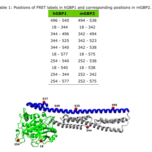
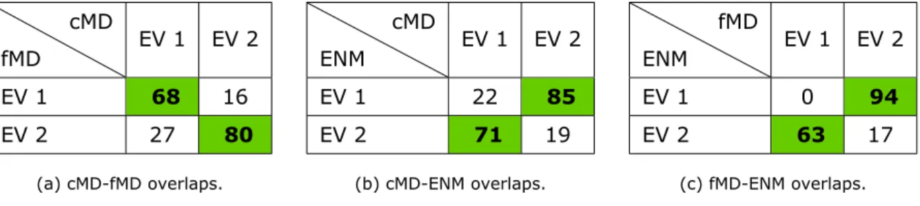
1 Positions of FRET labels in hGBP1 and corresponding positions in mGBP2. . . 24 2 Eigenvector overlaps between the first two collective modes for cMD, fMD and

ENM of nucleotide-free mGBP2. The largest overlap is highlighted in green with ``bold'' writing. . . 29 3 Distances between the given FRET pairs (hGBP1 counting of residues) of

distinct structures from the cMD simulation of

apo

-mGBP2 are compared to the experimental results from hpFRET measurements of hGBP1.⁽¹⁵⁾ The structure at 45.39 ns was chosen as it shows the greatest deviation from the initial state of the cMD simulation of

apo

-mGBP2 (RMSD of 7.9 Å) to cover the entire sampling. . . 35 4 Distances between the given FRET pairs (hGBP1 counting of residues) of

distinct structures from the cMD simulation of

apo

-mGBP2 are compared to the experimental results from hpFRET measurements of hGBP1.⁽¹⁵⁾ . . . 36

(9)

List of Figures

1 Structure model of mGBP2, which consists of three domains. The G domain is colored in green, the M domain in silver and the E domain in blue. . . 4 2 Salt bridges between the G domain and the

α

12/13-helix of

apo

-mGBP2 are

visualized, as well as possible changes in the

holo

-state (shown in red). The G domain of

apo

-mGBP2 is colored in green, the M domain in silver and the E domain in blue. . . 5 3 The G domain of

apo

-mGBP2 is displayed emphasizing the guanine cap, the

P-loop, the switch I and II regions, as well as the

α

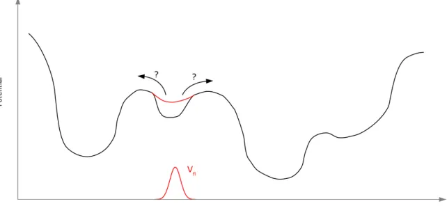
4'-helix (in glossy green).

The entire protein is shown in the background: the G domain is colored in transparent green, the M domain in transparent silver and the E domain in transparent blue. . . 6 4 The plot sketches the principle of conformational flooding. The red Gaussian

shaped flooding potential

V

_fl is added to the system's potential along user defined reaction coordinates suggested to reflect the essential dynamics of the protein. The figure was adapted from Lange et al.⁽⁶⁴⁾ . . . 12 5 The work-flow of fMD simulations is delineated. . . 19 6 The RMSD in Å is plotted against the simulation time in ns for fMD simulations

using different flooding strengths

E

_fl in kJ/mol. . . 21 7 The flooding potential

V

_fl in kJ/mol of an fMD simulation is plotted against the

simulation time in ns for a flooding strength of 10 kJ/mol. . . 21 8 FRET labeling positions are visualized in the mGBP2 model as red spheres

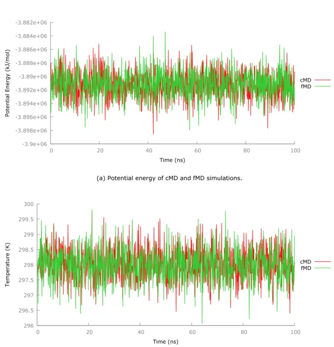
given the residue indices for hGBP1. The G domain of mGBP2 is shown in green, the M domain in silver and the E domain in blue. . . 24 9 The potential energy of

apo

-mGBP2 in kJ/mol (a) and the temperature of the

system in K (b) are plotted against the time in ns. The cMD simulation data is shown in red, the fMD data in green. . . 27 10 The RMSD of

apo

-mGBP2 (in Å) is plotted against the time in ns. The cMD

simulation is shown in red and the corresponding fMD simulation in green. . . 28 11 The first two collective modes of

apo

-mGBP2 are shown following the mode

order from PCA. The orange arrows mark the main direction of the motion of each mode. The G domain of mGBP2 is colored in green, the middle domain in silver and the E Domain in blue. . . 30 12 In the bottom half of the figure the relative B-factors from ENM (red), cMD

(green) and fMD (blue) of nucleotide-free mGBP2 are plotted against residue indices. The orange arrows relate the maxima to the corresponding flexible parts of the mGBP2 structure shown in the upper half of the figure. The G domain of mGBP2 is colored in green, the M domain in silver and the E domain in blue. Vertical gray lines separate the three domains in the B-factor plot. . . 31

(10)

List of Figures

13 The plot shows the projection of the structures of

apo

-mGBP2 from the cMD (red crosses) and fMD (green crosses) trajectories onto the first two principal components. The eigenvector factors are given in Å. . . 32 14 The figures illustrate the two states found for

apo

-hGBP1 from hpFRET exper-

iments. The G domain is shown in blue, the M domain in silver and the E domain in green color. The figures were gratefully obtained from the Seidel group⁽¹⁵⁾. . . 34 15 The plots show the distance distribution of hpFRET pairs during the cMD

simulation of

apo

-mGBP2. Distances are measured in Å with the bin width being 0.1 Åwhile the occurrence is given in %. The residue indices are based on the hGBP1 sequence. To obtain the corresponding amino acid in mGBP2, one has to subtract 2 starting from hGBP1 residue 165. . . 39 16 The figure visualizes the conformational space of the terminal part of the E

domain as sampled in the cMD simulation of nucleotide-free mGBP2. To this end, the terminal E domain conformations from the middle structure of each cluster are overlaid. The E domain is shown in blue, the M domain in silver and the G domain in green. . . 39 17 The potential energy of

holo

-mGBP2 in kJ/mol (a) and the temperature of the

system in K (b) are plotted against the time in ns. . . 41 18 The RMSD in Å is plotted against the time in ns for the fMD simulation of

nucleotide-bound mGBP2. . . 42 19 Non-bonded interaction energies in kJ/mol are plotted against the time in

ns for selected interactions of

holo

-mGBP2 during the fMD simulation. Non- bonded interactions consist of Coulomb interactions (red) and Lennard-Jones interactions (green). . . 44 20 The figures show the distributions for selected distances in

holo

-mGBP2 during

the fMD simulation. Distances are measured in Å with a bin width of 0.1 Å, while the occurrence is given in %. . . 45 21 Absolute B-factors in nm² are plotted against the residue indices. Data from

the fMD simulation of

apo

-mGBP2 is shown in red, the corresponding data of

holo

-mGBP2 in green. In the upper and lower parts of the figure B-factors are visualized in the mGBP2 structure. As underlying structure the middle structure of the biggest cluster of each simulation was chosen. Tube thickness and colors reflect the corresponding B-factors reaching from thin/blue (=0 nm², stiff) to thick/red (=1500 nm², flexible). . . 47 22 The conformational space of the G domain of

apo

- and

holo

-mGBP2 explored

in fMD simulations. The middle structures of selected regions resulting from cluster analyses are overlaid onto the structure of the

apo

-mGBP2 model. For the

apo

-state the G domain is shown in green, the M domain in silver and the E domain in blue. The

holo

-state is represented in red. . . 49

(11)

List of Figures

23 The conformational changes upon nucleotide binding are visualized for different structural motifs. The motifs of the

apo

-state are shown in green and the

holo

-state is colored in red. Conformations were obtained from cluster analysis and the middle structure of the highest populated cluster are shown for both

apo

- and

holo

-mGBP2. The entire structure of

apo

-mGBP2 is shown in the background in transparent green for the G domain, silver for the middle and blue for the E domain. The

holo

-state is colored in transparent red. The nucleotide GTP and the Mg²⁺ co-factor are colored in magenta. . . 50 24 The conformational space of the

α

13-helix in the GTP-bound state of mGBP2

is shown in red by overlaying all middle structures from cluster analysis at once. They are superimposed onto the initial structure of

apo

-mGBP2. The G domain is colored in green, the M domain in silver and the E domain in blue. . 51 25 Distance distributions for three salt bridges postulated between the G domain

and the terminal E domain for the

apo

-state are shown.

apo

-state data is given in red,

holo

data in green. . . 52 26 The figure sketches the conformational changes upon nucleotide binding where

the directions of resulting dynamics are indicated by orange arrows. The GTP binding site in the

apo

-state is shown in green and the

holo

-state is colored in red. Conformations were obtained from cluster analysis and the middle structure of the highest populated cluster of both states are overlaid. The entire structure of

apo

-mGBP2 is shown in the background in transparent green for the G domain, silver for the middle and blue for the E domain. The

holo

-state is colored in transparent red. The nucleotide GTP and the Mg²⁺

co-factor are colored in magenta. . . 53 27 The results of the H-bond analysis between the P-loop and the G4 motif are

shown. The upper part reflects the

apo

-state, the lower part the

holo

-state.

The strongest H-bonds are found between GLU50 and ARG181. . . 54 28 The H-bond between SER69 and SER246 in the

holo

-state is visualized. The

named residues are shown in red for the

holo

-state and in green for the

apo

-state. In the background the structure of the entire mGBP2 is displayed with red coloring for the nucleotide-bound protein, in green the G domain of

apo

-mGBP2, in silver the M domain and in blue the E domain. GTP and Mg²⁺

are visualized in purple. . . 55 29 Visualization of H-bonds, where the residues involved are shown in red for the

holo

-state and in green for the

apo

-state. In the background the structure of the entire mGBP2 is displayed with red coloring for the nucleotide-bound protein, green for the G domain of

apo

-mGBP2, silver for the M domain and blue for the E domain. GTP and Mg²⁺ are visualized in purple. . . 56

(12)

List of Figures

30 Visualization of the H-bonds between GTP and residues SER246, ARG238, ASP182, SER73, ARG48 and LYS51. These residues are shown in red. In the background the structure of the entire mGBP2 is displayed with red coloring for the nucleotide-bound protein, green for the G domain of

apo

-mGBP2, silver for the M domain and blue for the E domain. GTP and Mg²⁺ are visualized in purple. . . 57 31 Visualization of the coordination of Mg²⁺ by SER52. Residues are shown in

red. In the background the structure of the entire mGBP2 is displayed with red coloring for the nucleotide-bound protein, green for the G domain of

apo

- mGBP2, silver for the M domain and blue for the E domain. GTP and Mg²⁺ are visualized in purple. . . 57 32 The sequence alignment of hGBP1 and mGBP2 using the EMBOSS stretcher

tool for global pairwise alignment is shown. Green indicates identical sequence parts, yellow marks biochemically similar residues and red means no similarity.

Gray parts show gaps between the sequences. . . 69

(13)

List of Abbreviations

A acceptor

ARG arginine

ASP aspartic acid

CYS cysteine

D donor

ED essential dynamics

ENM elastic network model

EV eigenvector

FPS FRET-restrained positioning and screening

FRET Förster Resonance Energy Transfer

GBP guanylate binding protein

GDP guanosine-diphosphate

GLU glutamic acid

GLY glycine

GMP guanosine-monophosphate

GTP guanosine-triphosphate

H-bonds hydrogen bonds

hGBP1 human guanylate binding protein 1

hpFRET high performance Förster Resonance Energy Transfer H-REMD Hamiltonian replica exchange molecular dynamics

IFN-

γ

Interferon-

γ

kDa kilo dalton

LYS lysine

MD molecular dynamics

cMD classical molecular dynamics

fMD conformational flooding molecular dynamics

Mg magnesium

mGBP2 murine guanylate binding protein 2

NMA normal mode analysis

PBC periodic boundary conditions

PCA principal component analysis

PDB protein data bank

PV parasitophorous vacuole

QM/MM quantum mechanics/molecular mechanics

RESP restrained electrostatic potential

REMD replica exchange molecular dynamics

(14)

List of Abbreviations

RMSD root mean square deviation

RMSF root mean square fluctuation

RTB rotational-translational-block

SAXS small angle X-ray scattering

SER serine

T. gondii T oxoplasma gondii

THR threonin

VAL valine

VSV

vesicular stomatitis virus

(15)

Introduction

1 Introduction

1.1 Why study the murine Guanylate Binding Protein 2?

The murine Guanylate Binding Protein 2 (mGBP2) belongs to the family of Guanylate Bind- ing Proteins (GBP) and Atlastins of the Dynamin Superfamily of large GTPases⁽¹⁾. GBPs can make up up to 20% of the total cell proteome⁽²⁾. This family is more and more discovered to play an important role in the host defense against pathogenic infections⁽³⁾. Therefore there is great interest in unraveling the variety of processes, in which these proteins are involved, to determine the interactions between GBPs, signaling and effector molecules and thereby understand their importance during immune response. Furthermore, GBPs are seen as a model system to gain insights in the functioning of large GTPases⁽⁴⁾ and thereby of our immune system.

Highly up-regulated by interferon-

γ

(IFN-

γ

) GBPs are expressed through classical sec- ondary response genes⁽⁵⁾. Among others particularly mGBP2 is induced upon infection of mice with

Listeria monocytogenes

or

T oxoplasma gondii

(

T. gondii

)^{(6, 7)}.

T. gondii

is an obligate, intracellular parasite causing Toxoplasmosis in various warm blooded vertebrates^{(3, 8)}. The importance of its understanding arises from its serious course of disease in immune deficient humans^{(9, 10)} and its ability to act as a model system for other related parasites like

P lasmodia

a pathogen causing malaria⁽¹¹⁾. Via developing an infection model of mGBP2 after

T. gondii

contamination one aims at a better understanding of the immune response against

T. gondii

and thereby gaining new insights in the general functioning of the mammalian immune system.

1.2 State of the art in mGBP2 research Why apply Molecular Modeling to mGBP2?

Currently there is already some information on the structure and properties of mGBP2 available. As the sequence identity with the human Guanylate Binding Protein 1 (hGBP1) is 68%^(12--14), a structure model of mGBP2 was built based on the crystal structure of hGBP1 via homology modeling using SWISS model⁽³⁾. The nucleotide affinity of mGBP2 for the substrates Guanosine monophosphate (GMP), Guanosine diphosphate (GDP) and Guano- sine triphosphate (GTP) was studied and a mutant test series revealed important residues for nucleotide binding and hydrolysis, as well as for dimerization and tetramerization of mGBP2. Truncated mGBP2 models gave first insights in the specific functioning of the different protein domains and their interactions. Moreover, the localization of mGBP2 in vertebrates and the influence of biochemical processes like GTP hydrolysis and oligomerization were examined^{(3, 8, 14)}.

In addition, the structure and dynamics of hGBP1 were investigated via high-precision Förster Resonance Energy Transfer (hpFRET) and small angle X-ray scattering (SAXS) on

apo

-hGBP1 monomers⁽¹⁵⁾ and via electron paramagnetic resonance (EPR) and FRET on

(16)

1.3 The aim of this thesis Introduction

holo

-hGBP1 dimers⁽¹⁶⁾. This revealed the stable conformations of the monomeric protein and, together with X-ray structures of

holo

-hGBP1⁽¹⁷⁾, gave insights on structural changes during nucleotide binding, hydrolysis and dimerization. Given the high sequence identity between mGBP2 and hGBP1 these findings can be probably applied to mGBP2, which would be in agreement with the findings from extensive biochemical studies⁽³⁾.

Taken together, there is already knowledge about the structure of mGBP2, expected conformations, important residues for GTP binding, hydrolysis and oligomerization, but yet there is little known about the dynamics of mGBP2. Questions yet to be answered are, e.g., are there differences in the stable conformations of

apo

- and

holo

-mGBP2? How do the already revealed stable conformations interchange? What does the conformational space of functionally important residues look like? What is the dynamics upon nucleotide binding, which structural changes do lead to oligomerization and what happens during hydrolysis? Answering these questions is difficult to achieve but yet important to get a deeper understanding of the biologic functioning of mGBP2 and to develop models for immunological processes upon pathogenic infection. One possible approach is studying the murine Guanylate Binding Protein via molecular modeling as these tools are especially designed to explore the dynamics of a protein system.

1.3 The aim of this thesis

As the 67 kDa murine Guanylate Binding Protein 2^{(3, 14)}is rather large for molecular modeling, a first aim is to get a feeling for the handling of mGBP2 in modeling approaches; i.e., to determine appropriate modeling tools, test them for their ability to deliver new insights in the protein dynamics, and to discover whether there are particular difficulties with mGBP2.

A second aim is to unveil what kind of mGBP2 dynamics is predicted by molecular modeling and how does it compare to experimental results? Can the simulations reveal structural changes and pathways between stable conformations and what insights can be gained from looking in detail at the amino acids predicted to be important by experimental studies?

Finally, this thesis shall give a sound recommendation on how future work on mGBP2 via molecular modeling could proceed.

(17)

Background

2 Background

2.1 The murine Guanylate Binding Protein 2

2.1.1 Characteristics of mGBP2

The murine Guanylate Binding Protein 2 is a 67 kDa^{(3, 14)}, highly IFN-

γ

induced pro-

tein(5, 7, 8, 18--20) representing one of eleven murine isoforms^{(6, 13)}. It belongs to the family

of Guanylate Binding Proteins (GBPs) within the Dynamin Superfamily⁽¹⁾. Located in clus- ters on chromosome 3⁽⁶⁾, it is encoded in a 17.4 kb long gene via 1767 base pairs on 11 separate exons coding for 589 amino acids⁽³⁾.

mGBP2 has 68% sequence identity with hGBP1^{(12, 14)}. It shows a cooperative mechanism of GTP hydrolysis, which can be characterized as self-activation by oligomerization⁽¹⁴⁾. Binding to all guanosine phosphates (GTP, GDP and GMP)^{(12, 21)} it hydrolyzes GTP to GDP and GDP to GMP in two consecutive steps⁽¹⁴⁾. Whereas its nucleotide binding affinity is lower than that of the Ras family, the hydrolysis activity is much higher⁽³⁾. Mg²⁺ is an essential co-factor for hydrolysis⁽³⁾. The

apo

-state is stable as monomer and does not show any aggrega- tion⁽¹⁴⁾. Instead, mGBP2 multimerizes in a nucleotide-dependent manner: it dimerizes upon GTP binding and tetramerizes during the transitional state of hydrolysis⁽¹⁴⁾. Under cellular conditions this GTPase occurs as GTP-bound dimer⁽¹⁴⁾.

2.1.2 Biological Function of mGBP2

To date, there is little known about the biologic functions of GBPs⁽¹⁴⁾. mGBP2 predominantly localizes in vesicle like structures⁽¹⁴⁾ and is an important effector molecule in host defense against intracellular pathogens⁽¹⁴⁾. The interplay between GTP binding, oligomerization and GTP hydrolysis, as well as the isoprenylation motif of the C-terminus (see section 2.1.3) are prerequisites for the correct intracellular localization of mGBP2⁽³⁾. GBPs are assumed to have regulatory effects in cell adhesion and proliferation^{(22, 23)}. They are expected to be important in host resistance against bacteria such as

Listeria monocytogenes

and

M ycobacteria

^{(20, 24)}. mGBP2 is thought to have antiviral activities in NIH/3T3 fibroblasts after infection with

vesicular stomatitis virus

(VSV) or

encephalomyocarditis virus

^{(25, 26)}. It is supposed to have an inhibiting role for the cellular mobility of fibroblasts⁽²⁷⁾.

Pfeffer and co-workers studied in detail the role of mGBP2 upon infection with

T oxoplasma gondii

(

T. gondii

) in mice^{(3, 8, 14)}. It is up-regulated via IFN-

γ

through several pathways including B- and T-cells⁽⁸⁾. After recruiting to the parasitophorous vacuole (PV) of

T. gondii

⁽¹⁴⁾

its activity is assumed to be of reducing

T. gondii

replication⁽⁸⁾. To do so, it needs to act in synergism with other mGBPs⁽⁸⁾. It is suggested to form a kind of scaffold at the PV via oligomerization upon GTP hydrolysis to enable the assembly of other binding partners and co-factors, which then fulfill the antimicrobial functions⁽¹⁴⁾ and destroy the PV⁽⁸⁾.

(18)

2.1 The murine Guanylate Binding Protein 2 Background

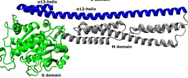
G domain

E domain α13-helix

α12-helix

M domain

Figure 1: Structure model of mGBP2, which consists of three domains. The G domain is colored in green, the M domain in silver and the E domain in blue.

2.1.3 Structure of mGBP2 and Hydrolysis Model

Since up to now only the crystal structure of hGBP1 has been solved, the structure of mGBP2 is not known yet. However, given the high sequence identity between hGBP1 and mGBP2 it was possible to predict the mGBP2 structure via homology modeling using the SWISS-MODEL server^{(28, 29)}. The mGBP2 overall structure is expected to be a three domain structure consisting of a Ras-like G domain, which is the catalytic GTPase domain, a middle domain (M domain) built of two bundles of

α

-helices and the long

α

-helical E domain spanning the complete backside of the protein⁽³⁾ (see figure 1).

The E domain consists of the protein spanning

α

12-helix and, after a turn, the

α

13-helix near the C-terminus of the protein. At the C-terminus the CAAX sequence is located (amino acids 586-589), which is a recognition motif for farnelylization or geranylgeranylization en- zymes. This enzyme will attach an isoprene at the X position. Thereby the sub-cellular localization of mGBP2 is determined and interactions with a membrane are enabled⁽³⁾. The E domain is stabilized via salt bridges between the G domain and the

α

12/13-helices. They are visualized in figure 2.

Apart from some deviations the G domain of mGBP2 shown in figure 3 is mainly conserved from the canonical Ras structure⁽¹⁴⁾. It includes the four motifs (G1 G4) where G1 and G3 are fully conserved⁽³⁾. The G1 motif (P-loop) is responsible for binding GTP via hydrogen bonds (H-bonds) to

α

-,

β

- and

γ

-phosphate, the hydroxy groups of serine (SER) and threonin (THR) coordinate Mg²⁺ in the

holo

-state. The so-called switch I region (G2 motif) is important during hydrolysis as it coordinates the reacting water molecule and Mg²⁺, and shields the binding pocket from the solvent. Just as the switch I region the switch II region (G3 motif) undergoes large conformational changes upon hydrolysis. Its THR and glycine (GLY) residues coordinate the GTP

γ

-phosphate⁽³⁾. The G4 motif contains the recognition

(19)

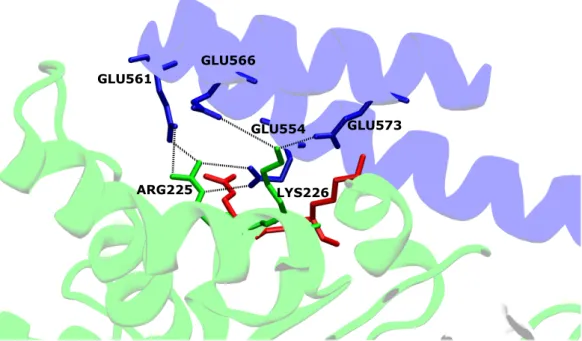
GLU561

GLU566

GLU573 GLU554

ARG225 LYS226

Figure 2: Salt bridges between the G domain and the

α

12/13-helix of

apo

-mGBP2 are visualized, as well as possible changes in the

holo

-state (shown in red). The G domain of

apo

-mGBP2 is colored in green, the M domain in silver and the E domain in blue.

sequence for the guanine base and is only conserved in form of a reduced RD motif from the canonical Ras structure⁽³⁾. Aspartic acid (ASP) stabilizes GTP and GDP via H-bonds, two more amino acids preserve the structure of the nucleotide binding pocket via contacting the P-loop⁽³⁾. There is one more exclusive motif found for hGBP1 called the guanine cap. It shows large conformational changes upon nucleotide binding and seems to be important for the stable binding of GTP/GDP, hydrolysis and dimerization⁽³⁰⁾. This structural element is also predicted for mGBP2⁽³⁾. Furthermore, from crystal structures of

holo

-hGBP1⁽¹⁷⁾ it is seen, that the

α

4'-helix also severely changes its conformation during GTP binding⁽³¹⁾. From mutation studies of arginine (ARG) 48, lysine (LYS) 51, ASP 182 and glutamic acid (GLU) 99 the important amino acids carrying the specific functions of the G1-G4 motifs were resolved⁽³⁾. ARG 48 acts as the so-called ``arginine finger'' which is important for the hydrolysis activity of mGBP2 and stabilizes the mGBP2 dimer⁽¹⁴⁾. With its positively charged side chain LYS 51 supports the binding of GTP via

β

- and

γ

-phosphate interactions and is essential for a cooperative hydrolysis mechanism. It preserves the P-loop structure by forming H-bonds to THR 98 (switch I)⁽³⁾. The specificity for guanine bases is ensured by ASP 182 in the G4 motif^{(3, 14)}. GLU 99 (switch II) might stabilize the transition state of hydrolysis and thereby accelerate the phosphate cleavage by conformational changes^{(3, 14)}.

The mechanism of hydrolysis is not entirely solved yet but differs from the mechanisms in the Ras and G_α family⁽³⁾. Upon GTP binding and subsequent hydrolysis to GDP, large conformational changes occur in hGBP1. The closure of the binding pocket by a large conformational change of the guanine cap enables stable nucleotide binding and initiates the dimerization process through polar interactions with the switch regions forming head

(20)

guanine cap α4'-helix

switch I switch II P-loop

Figure 3: The G domain of

apo

-mGBP2 is displayed emphasizing the guanine cap, the P-loop, the switch I and II regions, as well as the

α

4'-helix (in glossy green). The entire protein is shown in the background: the G domain is colored in transparent green, the M domain in transparent silver and the E domain in transparent blue.

to head dimers⁽³⁰⁾. The

α

6-helix is assumed to play a critical role during this process⁽³²⁾. It is at 80% identical between hGBP1 and mGBP2 and is therefore likely to be involved in the dimerization of mGBP2, too⁽³⁾. Dimerization leads to a self-activation of the hydrolysis making it a cooperative mechanism.

Like for hGBP1⁽³¹⁾, during hydrolysis of GTP to GDP the

α

4'-helix of the G domain seems to mediate a force to the E domain of mGBP2 resulting from structural changes in the active site⁽³⁾. This could unveil a surface for further interactions with other proteins, e.g., causing tetramerization by dimerization of two mGBP2 dimers⁽³⁾. This tetramerization is only possible during the transitional state of GTP hydrolysis⁽³⁾. Because of the high sequence identity between hGBP1 and mGBP2, similar mechanisms are expected for both proteins.

Via truncation studies it was shown that for its biological functions all three mGBP2 domains are essential⁽³⁾. The G and E domain have direct contacts⁽³⁾ and it is proposed that the E domain inhibits hydrolysis of externally bound GDP because conformational changes from the first cleavage step are missing⁽³⁾. Whereas the E domain is important for the recruitment of mGBP2 to the PV of

T. gondii

and membrane attachment, the G domain regulates this process. It ensures that mGBP2 is only activated after IFN-

γ

stimulation by unmasking a binding motif in the E domain during hydrolysis as explained above⁽⁸⁾. This is in line with the finding that GTPase activity is needed for assembly at the PV⁽¹⁴⁾.

(21)

2.2 Elastic Network Models Background

2.2 Elastic Network Models

Elastic Network Models (ENM) provide a simplified, low-resolution model of a biomolecule (in particular proteins) intending to describe its overall large-scale, low-frequency motions⁽³³⁾. The biomolecule is modeled via a three-dimensional elastic network build up of beads representing a user-defined group of atoms and connecting beads below a certain predefined cutoff via springs⁽³⁴⁾.

Taking a protein as example, these beads are often represented by the C_α-atoms and all C_α-atoms closer than, e.g., 10 Å from each other are connected via springs. This leads to a very simple energy function, which is only dependent on these elastic connections.

There are different approaches to the spring descriptions, for example, either using a single-parameter Hookean potential like suggested by Tirion⁽³³⁾ or a more sophisticated description like the Hinsen model^{(35, 36)}. Equation (1) shows the potential

V

_p

(r

_a

, r

_b

)

as proposed by Tirion⁽³³⁾:

V

p

(r

a

, r

b

) = X

|r⁰_a,b|<rc

C

2 |r

a,b

| − |r

_a,b⁰

|

2

(1)

with parameter

C

being a definable force constant describing all interactions,

r

_a,b

≡ r

_a

− r

_b

denoting the distance vector between atoms

a

and

b

, the superscript

0

indicates the starting configuration, and the sum runs only over atom pairs being closer than a predefined cutoff

r

c.

By applying Normal Mode Analysis (NMA) to equation (1) (meaning diagonalizing the matrix of second derivatives of the potential energy, i.e., the Hesse matrix)⁽³³⁾ the system's eigenvectors (EV) and corresponding eigenvalues are obtained. The eigenvalues are directly related to the frequencies of the normal modes. The resulting eigenvectors are sorted according to growing frequency, where for molecules with three degrees of rotational freedom (valid for all biomolecules) the first six eigenvectors represent the translational and rotational so-called trivial modes. The interesting part are the non-trivial low-frequency modes representing the system's large-scale conformational changes. It was shown, that the temperature factors (so-called B-factors) predicted from ENMs are in good correlation with crystallographic data and that specific conformations are recovered⁽³⁷⁾.

One has to be aware that applying NMA to the ENM does only make sense, if the ENM describes an equilibrium state of the represented biomolecule meaning that it reflects an energy minimum⁽³⁸⁾. That is because the simple ENMs are basically a harmonic approx- imation of the biomolecule's potential function and applying NMA defines the provided structure as the energy minimum of this harmonic potential. This already delineates the only requirement needed as input to build an ENM: A structure of the biomolecule at an equilibrium state must be available (e.g., a crystal structure). ENMs save the costly energy minimization step which would be necessary when doing NMA with a standard biomolecular

(22)

2.3 Molecular Dynamics Simulations Background

force field. Furthermore, these models speed up the matrix diagonalization remarkably by only considering a subset of atoms, e.g., the C_α-atoms⁽³⁴⁾. Taken together this leads to the clear advantage of ENMs: They provide key insights into large-scale conformational, often function-related motions of proteins which are often computationally demanding to obtain via classical Molecular Dynamics (cMD) simulations, especially for large biomolecules. And as explained, this is achieved at almost no computational expense: The mGBP2 protein studied in this work consists of 573 residues. Building a C_α-model leads to an ENM with 573 beads, providing NMA results in less than 5 minutes on four 2.53 GHz cores.

2.3 Molecular Dynamics Simulations

2.3.1 Newton's equation of motion Leap Frog algorithm

The underlying foundation of molecular dynamics (MD) simulations is Newton's Equation of motion (2)^{(39, 40)}:

F

_i

(t) = m

_i

v ˙

_i

(t)

(2)

It says that the force

F

_i currently acting on particle

i

and its mass

m

_i solely determine the acceleration of particle

i

. Knowing the current position of particle

i

and its velocity

v

i one can obtain its future position via integrating over a time step

∆t

. In MD simulations this is implemented by iteratively updating the forces on particle

i

and then calculating the newly resulting velocities and positions for a defined time step

∆t

.

The leap-frog algorithm⁽⁴¹⁾ is one widely used algorithm to iteratively integrate Newton's differential equation (2). Its name arose due to its characteristic that positions and velocities always jump over each other like leapfrogging. Velocities are updated at each half time step

∆t/2

and positions at each time step

∆t

.

v

_i

t − ∆t 2

= x

_i

(t) − x

_i

(t − ∆t)

∆t

⁽³⁾

v

_i

t + ∆t 2

= x

_i

(t + ∆t) − x

_i

(t)

∆t

⁽⁴⁾

Equation (3) describes the latest known velocity, equation (4) the future velocity, where

v

_i

denotes the velocity and

x

_i the position of particle

i

. In case of all-atom MD simulations particle

i

represents one atom.

∆t

defines the time step between iterations and

t

indicates the current time. By expanding equation (4) in a Taylor series, the future velocity can be obtained:

v

_i

t + ∆t 2

≈ v

_i

t − ∆t 2

+ ∆t F

_i

(t)

m

⁽⁵⁾

(23)

with

m

_i being the mass of and

F

_i the force acting on atom

i

. Solving equation (4) for

x

_i

(t + ∆t)

yields the future position of atom

i

:

x

i

(t + ∆t) = x

i

(t) + ∆tv

i

t + ∆t 2

(6)

One has to be aware that the resulting position leads to an error of order

O

(

∆t

⁴) and the velocity to an error of order

O

(

∆t

²) because of stopping the Taylor expansion (5) after the second term.

2.3.2 Force Fields Amber ff99SB-ILDN

The leap-frog algorithm (see section 2.3.1) itself does not yet allow us to compute new positions and velocities for a given atom. The force acting on each atom has to be determined first to solve equation (5). It is calculated via the first derivative of the potential energy:

F

_i

= ∂V (R)

∂x

_i ⁽⁷⁾

with

V (R)

denoting the potential energy which depends on

R

, i.e., all positions of the

N

atoms composing the system and

x

i is one of the three Cartesian coordinates of atom

i

.

In MD simulations force fields are used to describe the potential energy of a simulation system. Various implementations exist to account for this need, which can be divided into knowledge-based and physics-based force fields⁽⁴²⁾. The first derive the potential energy from statistics and experimental data, whereas the latter account for the interactions between particles via a physical description. Physics-based force fields can be further divided into all-atom and coarse-grained force fields. Whereas all-atom force fields represent the highest level of theory explicitly describing each atom of the system, coarse-grained models group several atoms into one bead to reduce the computational effort.

Within these categories one can choose between many different models, each having individual strengths and weaknesses, which, e.g., can be overstabilization of

α

-helices, salt-bridges or protein oligomers. This is due to the fact that force fields represent empirical descriptions of the biomolecules, which involve many parameters which where obtained in a complex parametrization procedure^(43--46). Well known all-atom force fields are the CHARMM^(47--49), GROMOS^{(50, 51)} and AMBER^(52--54) force fields. Choosing the correct level of theory and force field is a very sensitive decision immensely depending on the simulation problem one wants to describe. When analyzing simulation results one has to carefully consider the impact of the force field applied to the problem of interest⁽⁴²⁾.

The mutual foundation of all physics-based all-atom force fields is the systematic derivation

(24)

of the system's potential energy based on equation (8):

V = V

^bond

+ V

^elec

+ V

^vdW (8)

V

^bond accounts for the bonded interactions, while the non-bonded interactions arise from electrostatic

V

^elec and van der Waals

V

^vdW interactions⁽⁴⁵⁾. One example for such a physics- based all-atom force field is the Amber ff99 force field given in equation (9)⁽⁵²⁾:

V

^ff99

= X

i∈bonds

K

_r,i

(r

_i

− r

_i⁰

)

²

+ X

i∈angles

K

_θ,i

(θ

_i

− θ

_i⁰

)

²

+ X

i∈dihedrals

V

_n

2 [1 + cos(nφ

_i

− γ)]

+ X

i∈atoms

X

j>i

q

i

q

j

r

_ij

+ X

i∈atoms

X

j>i

A

ij

r

_ij¹²

− B

ij

r

_ij⁶

(9)

Here, the first three terms account for the bonded interactions

V

^bond whereas the last two terms describe the non-bonded electrostatic

V

^elec and van der Waals

V

^vdW interactions.

K

_r,i,

K

_θ,i and

V

_n denote the force constants for bond vibrations, angle bending and dihedral torsions, the subscript

0

marks the corresponding equilibrium geometry. For the non-bonded interactions,

r

_ij represents the distance between atoms

i

and

j

with

q

_i and

q

_j

being their partial charges.

A

_ij and

B

_ij correlate to their van der Waals radii. The last term describing the van der Waals interactions has the form of a Lennard-Jones potential. The parameter

denotes the dielectric constant.

The Amber ff99 force field has been re-parametrized and thereby improved twice over time: First it was replaced by the Amber ff99SB force field introduced by Hornak et al.⁽⁵³⁾, which improved the backbone

φ/ψ

dihedral terms in order to obtain a better balance between

α

-helical and

β

-sheet structures. The last update was by Lindorff-Larsen et al.⁽⁵⁴⁾ to improve amino acid side-chain torsion potentials of isoleucine, leucine, aspartate and asparagine (I,L,D,N) of the Amber ff99SB force field leading to the Amber ff99SB-ILDN force field.

For the calculation of the potential energy as defined in equation (9) two ingredients are needed: Atom coordinates which are being provided during the MD simulation and force field parameters. The latter are of utmost importance and the core problem when developing a new force field. As a force field is generally not intended to describe a special atom or molecule but, for example, any protein, these parameters have to be carefully derived from ab-initio calculations at the quantum-mechanics level and fitting to experimental target data like vibrational spectra and solvation free energies⁽⁴⁵⁾. They highly determine the quality of the force field and the achievable results in MD simulations.

(25)

2.3.3 Enhanced Sampling Simulations Flooding

A main concern of molecular dynamics simulations is to achieve a sufficient sampling of the conformational space to derive statistically significant results^{(55, 56)}, which becomes more critical with growing degrees of freedom. Therefore a vast effort is taken to develop advanced techniques which enhance the sampling of MD simulations, which widely differ in their theoretical foundations and approaches.

Adcock and McCammon proposed to summarize the developments into three, partially over- lapping classes: methods explicitly modifying the potential energy surface, methods using non-Boltzmann sampling, and methods accelerating the sampling of particular degrees of freedom while slowing down others⁽⁵⁷⁾. Into the first class they count, for example, the deflation method⁽⁵⁸⁾, umbrella sampling⁽⁵⁹⁾, local elevation⁽⁶⁰⁾, potential smoothing⁽⁶¹⁾, conformational flooding^(62--64), hyperdynamics^{(65, 66)}, and accelerated MD⁽⁶⁷⁾. Following Bernardi et al.

also metadynamics⁽⁶⁸⁾ should be added here⁽⁵⁶⁾. The main characteristic of this group is to enlarge the sampling efficiency by reducing the simulation time spent at local minima and thereby to prevent the simulation from being stuck at a local minimum. The second group, in principle, follows the same idea. It includes different sampling methods like simulated annealing⁽⁶⁹⁾ and replica exchange MD (REMD)^{(70, 71)}. They differ from the first group in that they leave the energy surface unchanged. One of the most established methods from the third group is the SHAKE algorithm⁽⁷²⁾, which is widely used to constrain bond lengths during MD simulations.

In this work the conformational flooding technique⁽⁶⁴⁾ as implemented in the GROMACS software package^(73--78) is applied. Its basic principle is to destabilize a local minimum structure by adding a Gaussian shaped flooding potential

V

_fl to the potential energy surface along user-defined so-called collective coordinates (see figure 4). When simulating proteins, these collective coordinates are typically chosen such that they reflect the Essential Dynamics (ED) of the protein. ED represent the overall large-scale motions of a system emphasizing the function-related dynamics. They may be obtained via Principal Compo- nent Analysis (PCA)⁽⁷⁹⁾ from a preceding MD simulation or also via NMA from an ENM (as introduced in section 2.2).

The destabilization of the local minimum structure is achieved through adding a flooding potential

V

_fl (equation (10)) along the

a priori

defined

m

collective coordinates.

V

_fl

(c

₁

, ...c

_m

) = E

_fl

exp

"

− k

_B

T 2E

_fl

m

X

j=1

λ

_j

c

_j

− c

⁽⁰⁾_j

2

#

(10)

Here,

k

_B denotes the Boltzmann-constant,

T

the simulation temperature, and

λ

_j desig- nates a curvature reflecting the eigenvalue corresponding to

c

_j, the

j

-th eigenvector of the

m

user-defined collective coordinates.

c

⁽⁰⁾_j describes the center of the flooding potential of eigenvector

j

.

V

_fl can be chosen to be constant throughout the simulation via a user- defined fixed flooding strength

E

_fl or be adapted by defining a target destabilization free

(26)

Potential

Reaction Coordinate

? ?

V_fl

Figure 4: The plot sketches the principle of conformational flooding. The red Gaussian shaped flooding potential

V

_fl is added to the system's potential along user defined reaction coordinates suggested to reflect the essential dynamics of the protein. The figure was adapted from Lange et al.⁽⁶⁴⁾

energy

∆F

₀ and updating the corresponding flooding strength

E

_fl⁽ⁱ⁺¹⁾ at each time step

i

(equation (11)).

E

_fl⁽ⁱ⁺¹⁾

≡ E

_fl⁽ⁱ⁾

+ ∆t τ

∆F

₀

− ∆F

⁽ⁱ⁾

(11)

∆t

is the step size used for the MD simulation and

τ

the user-defined time constant, which controls the update frequency of

E

_fl.

∆F

⁽ⁱ⁾ and

E

_fl⁽ⁱ⁾ are the destabilization free energy and flooding strength at the current time step

i

, respectively.

The advantage of the flooding technique is that it allows an unbiased sampling of the conformational space towards any direction by only driving the system away from local minimum states. Apart from the required collective coordinates from PCA or NMA there is no further prior information, like transition pathways or product states, needed.⁽⁶⁴⁾

(27)

Methods

3 Methods

3.1 mGBP2 structure models for molecular modeling

3.1.1 Nucleotide-free model of mGBP2

To date, the only GBP structure that has been solved is the one of hGBP1⁽⁸⁰⁾ (protein data bank (PDB)⁽⁸¹⁾ search as of 17^thof September, 2015). As mGBP2 shows a sequence identity of 68% with hGBP1^{(12, 14)}, the crystal structure of the

apo

-state of the latter (PDB entry 1DG3)⁽⁸⁰⁾ was used by Kravets⁽³⁾ to build a model of

apo

-mGBP2 via homology modeling using the SWISS-MODEL server available athttp://swissmodel.expasy.org/^{(28, 29)}. Thereby a structural model of mGBP2 covering amino acids 6 to 578 was obtained. The last eight amino acids including the CAAX sequence are missing in this model as the structure of the corresponding hGBP1 residues could not be resolved⁽³⁾. The structure model obtained from Kravets⁽³⁾was the basis for all modeling of the

apo

-state of mGBP2 done in this work.

3.1.2 GTP bound model of mGBP2

The crystal structure of the G domain of

holo

-hGBP1 bound to the non-hydrolyzable GTP analogue GppNHp (PDB entry 2BC9)⁽¹⁷⁾ served as precursor to obtain a homology model of the

holo

-state G domain of mGBP2 using the same method as explained above (section 3.1.1). To be able to simulate the complete

holo

-state of mGBP2, the M and E domains had to be added to the nucleotide-bound G domain. To this end, the

holo

-state G domain model (also obtained from Kravets⁽³⁾) was used to replace the G domain of the existing

apo

-state model. To do so, the latter was cut at the

ψ

-angle of valine (VAL) 286 and amino acids 6 to 286 were replaced by the

holo

-state G domain model. To prevent the loop from residue 155 to 170 from being wrapped around the

α

12-helix, the bond between the C and C_α-atoms of residue 481 was slightly stretched to move the

α

12/13-helices a little apart from the G domain. All these transformations were done using the VMD software⁽⁸²⁾. Furthermore, the nucleotide GTP and the Mg²⁺ co-factor had to be added. To do so, the resulting structure was further processed with the free version of the Maestro program⁽⁸³⁾. The

holo

-state model was loaded together with the coordinates of Mg²⁺ and GDPxAlF3

obtained from the crystal structure of the GDPxAlF3 bound hGBP1 G domain (PDB entry 2B92)⁽¹⁷⁾. AlF3 was removed and a phosphate group was attached to the

β

-phosphate of the existing GDP. The

γ

-phosphate was added in a way to avoid atom clashes and to be in a reasonable position relative to important protein residues, in particular to LYS51 and the Mg²⁺ co-factor as described by Kravets (see figure 1.13 of Kravets' dissertation⁽³⁾ and section 2.1.3 of this work). The GTP structure was protonated to mimic the physiological pH value of 7.4 (the protonation state was derived from the GTP structure with PDB code 2KSQ, which was obtained using solution NMR at a pH value of 7⁽⁸⁴⁾) giving it an overall charge of

−4

. It was then pre-optimized according to the protein and co-factor environment within Maestro, which makes use of the OPLS_2005 force field⁽⁸⁵⁾.

The here described procedure is in line with previous work from others⁽⁸⁶⁾. The obtained

(28)

3.2 Elastic Network Models Methods

coordinates defined the input structure for the simulations of the

holo

-state which was first energy minimized in order to optimize the geometry, especially to relax the artificially enlarged bond in residue 481, using the GROMACS package. Details on the setup and minimization and MD simulation protocols are given in section 3.3.1.

3.1.3 Derivation of GTP force field parameters

As there are no standard parameters implemented in the Amber ff99SB-ILDN force field for GTP in GROMACS, they were taken from the work of Meagher et al.⁽⁸⁷⁾. A similar procedure for the incorporation of the named GTP parameters in GROMACS was recently published by Gao and Eriksson⁽⁸⁶⁾. The still missing partial atomic charges of GTP were derived following the procedure of the Amber ff99SB-ILDN force field parametrization using the restrained electrostatic potential (RESP) method⁽⁸⁸⁾ at the Hartree-Fock theory level applying the 6- 31G* basis set after prior geometry optimization of GTP using the B3LYP functional with the 6-31G* basis set. These quantum chemical calculations were done using the Gaussian 09 program⁽⁸⁹⁾ following the recommendations of the Department of Theoretical Chemistry of the Lund University (available athttp://www.teokem.lu.se/ ulf/Methods/resp.html) and are in line with procedures described elsewhere^{(90, 91)}. Finally a complete parameter file for use in GROMACS was built by combining the derived RESP charges and the GTP parameters published by Meagher et al.⁽⁸⁷⁾ in Amber frcmod file format via the antechamber^{(92, 93)} and tleap⁽⁹⁴⁾ tools available within the AmberTools15 software package⁽⁹⁵⁾. The resultingprmtop and prmcrd files were converted to GROMACS topology and coordinate files using the ACpype tool⁽⁹⁶⁾.

3.2 Elastic Network Models

3.2.1 Software for ENM calculations and employed parameters

All elastic network models applied in this work were build using the

∆∆

PT toolbox de- veloped by Rodgers et al.⁽⁹⁷⁾ The source code is available at http://sourceforge.net/

projects/durham-ddpt/ and can be installed at a local machine free of charge. For setting up the ENMs, structure files in pdb file format were parsed to the toolbox and coarse grained models only considering C_α-atoms without mass-weighting were built, using a distance cutoff of 10 Å for spring connections applying a single-parameter Hookean potential with a force constant of 1 kcal/mol/Å². These settings reflect a standard procedure as described elsewhere⁽³⁴⁾. Normal mode analysis was fully performed with the DIAGSTD procedure of

∆∆

PT not applying the rotational-translational-block (RTB) approach⁽⁹⁸⁾. The results were further analyzed using the FREQ/EN tool at a temperature of 298 K, the RMS/COL tool considering all non-trivial mode eigenvectors and the NMWIZWT program for normal mode visualization.

(29)

3.3 Molecular Dynamics Simulations Methods

3.2.2 Verifying the choice of ENM software and ENM parameters

To check the influence of different parameters and levels of coarse graining, tests of different ENMs were performed. Here, all-atom ENMs and C_α-ENMs with residue mass weighting were considered. Visual inspection of the resulting three non-trivial normal modes with smallest eigenvalues using the VMD software, comparison of the overlap between corresponding eigenvectors (using the OVERLAP procedure of

∆∆

PT described in section 3.4.2) and the mode collectivity did not show any major differences. But it was seen that the amplitude of motions declined with increasing model accuracy, which is not favored.

As many different ENM software like the elNèmo⁽⁹⁹⁾, WebNMA⁽¹⁰⁰⁾ and ADENM⁽¹⁰¹⁾ web servers and others are available, it was further tested whether they produce different results. Building standard C_α-ENMs and doing NMA with these web servers showed in general a high agreement in results. These were examined following the same procedure as mentioned above. Only the WebNMA web server differed from the others, yielding a reduced eigenvector overlap of 93-96% compared to almost 100% for the others.

The findings of the tests performed are in line with the results from Kitao et al.: The choice of ENM and the level of theory (e.g., describing the potential via all-atom force fields vs. a simple single-parameter Hookean potential) is seen to be uncritical for the low frequency collective motions^{(102, 103)}. Therefore, the software choice for ENMs can be done according to user convenience. Here the

∆∆

PT has clear advantages compared to the others tested, because it allows to control any single parameter and setting when building the ENM. Furthermore, the calculations are all easy to follow, while it turned out to be rather difficult for the web servers to follow, what was actually done during building the ENM and performing the NMA, giving the impression of being a ``black box''. Finally, the

∆∆

PT toolbox comes with many additional features like visualization of normal modes, it is easy to install and use and it is distributed with a detailed documentation.

3.3 Molecular Dynamics Simulations

3.3.1 Free Simulations

Classical Molecular Dynamics (cMD) simulations were performed using the GROMACS^(73--78) software package available as free download athttp://www.gromacs.org/ and applying the Amber ff99SB-ILDN force field^(52--54). The mGBP2

apo

-state model was solvated with the explicit TIP3P water model⁽¹⁰⁴⁾ in a dodecahedron box employing periodic boundary conditions (PBC) with a 10 Å minimum distance from any mGBP2 atom to the closest box edge.

Na⁺was added to neutralize the system and the temperature was set to 298 K. Missing hy- drogens were added using the interactivepdb2gmxcommand to mimic the physiological pH of 7.4. To decide on the protonation states of amino acids the propka31 tool^{(105, 106)}was used to predict pKa values. Amino acids with a pKa value greater than pH=7.4 were assigned to be protonated, in turn those with a pKa lower than pH were decided to be not protonated.

(30)

3.3 Molecular Dynamics Simulations Methods

After setting up the system, an energy minimization was performed using the steepest descent algorithm with a maximum force tolerance of 500 kJ/mol/nm on any atom and a maximum number of steps of 10,000. Further details can be seen in the

apo

-state minimization mdp file in the appendix (section 6.1.1). Next, the system was equilibrated for 100 ps using the leap-frog integrator⁽⁴¹⁾ (compare section 2.3.1), the Berendsen barostat⁽¹⁰⁷⁾ ensuring a pressure of 1 bar and the velocity-rescale thermostat⁽¹⁰⁸⁾ maintaining a temperature of 298 K. Protein heavy atom coordinates were restrained. Velocities were generated according to a Maxwell-Boltzmann distribution at 298 K. Finally, the MD production run was performed for 100 ns applying the Nose-Hoover thermostat^{(109, 110)}and the Parinello-Rahman barostat^{(111, 112)}at the before mentioned temperature and pressure. Further equilibration and production run specifications are given in the appendix (section 6.1.2 and 6.1.3).

To set up the

holo

-state simulation system for the GTP bound model of mGBP2 described in section 3.1.2, the aforementioned procedures for the

apo

-state system were followed including a new pKa value prediction with propka31. However, slight changes to the settings described above had to be made for the

holo

-state simulations. For a successful energy minimization, GROMACS had to be run in double precision mode. The initial energy step size was enlarged to 0.1 Å. Two equilibration runs were used, the first for velocity generation while restraining protein heavy atom coordinates, as well as GTP and Mg²⁺, the second only restraining protein heavy atoms, which allowed GTP and Mg²⁺ to find their optimal position in the binding pocket. For temperature coupling, two groups were used:

one including protein, GTP and Mg²⁺, and the other one with water and ions. The MD production runs were performed with the same temperature coupling groups as during equilibration. For later analysis the energy terms were split into two groups, protein and GTP. All specifications can be viewed in the appendix in sections 6.1.1, 6.1.2 and 6.1.3.

3.3.2 Enhanced Sampling Simulations Flooding

Enhanced sampling simulations were performed using the flooding tool⁽⁶⁴⁾ implemented in GROMACS for both the

apo

- and the

holo

-state. When specified in themdruncommand this tool is called by GROMACS' main MD engine within itsedsammodule and accounts for the force calculations due to the additional flooding potential. The needed input parameters are parsed to GROMACS via the edi input file which can be generated with GROMACS' make_ediprogram⁽⁶⁴⁾.

Enhanced sampling simulations shall speed up the sampling of collective essential dynamics. Because the simulation time needed to receive a converged principal component analysis and thereby a sufficient description of reaction coordinates for flooding is unclear, a coordinate derivation via NMA was preferred. Here, elastic network models provide an efficient possibility and an appropriate level of theory for the calculation of normal modes and the determination of flooding coordinates. As an ENM and subsequent NMA defines the input geometry as the energy minimum, the reaction coordinates of the flooding potential