Random walks and electric networks

Random walks and electric networks

Peter G. Doyle J. Laurie Snell Version dated 5 July 2006

GNU FDL

Acknowledgement

This work is derived from the book Random Walks and Electric Net- works, originally published in 1984 by the Mathematical Association of America in their Carus Monographs series. We are grateful to the MAA for permitting this work to be freely redistributed under the terms of the GNU Free Documentation License.

∗Copyright (C) 1999, 2000, 2006 Peter G. Doyle and J. Laurie Snell. Derived from their Carus Monograph, Copyright (C) 1984 The Mathematical Association of America. Permission is granted to copy, distribute and/or modify this document under the terms of the GNU Free Documentation License, as published by the Free Software Foundation; with no Invariant Sections, no Front-Cover Texts, and no Back-Cover Texts.

Preface

Probability theory, like much of mathematics, is indebted to physics as a source of problems and intuition for solving these problems. Unfor- tunately, the level of abstraction of current mathematics often makes it difficult for anyone but an expert to appreciate this fact. In this work we will look at the interplay of physics and mathematics in terms of an example where the mathematics involved is at the college level. The example is the relation between elementary electric network theory and random walks.

Central to the work will be Polya’s beautiful theorem that a random walker on an infinite street network in d-dimensional space is bound to return to the starting point when d= 2, but has a positive probability of escaping to infinity without returning to the starting point when d≥3. Our goal will be to interpret this theorem as a statement about electric networks, and then to prove the theorem using techniques from classical electrical theory. The techniques referred to go back to Lord Rayleigh, who introduced them in connection with an investigation of musical instruments. The analog of Polya’s theorem in this connection is that wind instruments are possible in our three-dimensional world, but are not possible in Flatland (Abbott [1]).

The connection between random walks and electric networks has been recognized for some time (see Kakutani [12], Kemeny, Snell, and Knapp [14], and Kelly [13]). As for Rayleigh’s method, the authors first learned it from Peter’s father Bill Doyle, who used it to explain a mysterious comment in Feller ([5], p. 425, Problem 14). This comment suggested that a random walk in two dimensions remains recurrent when some of the streets are blocked, and while this is ticklish to prove probabilistically, it is an easy consequence of Rayleigh’s method. The first person to apply Rayleigh’s method to random walks seems to have been Nash-Williams [24]. Earlier, Royden [30] had applied Rayleigh’s method to an equivalent problem. However, the true importance of Rayleigh’s method for probability theory is only now becoming appre- ciated. See, for example, Griffeath and Liggett [9], Lyons [20], and Kesten [16].

Here’s the plan of the work: In Section 1 we will restrict ourselves to the study of random walks on finite networks. Here we will establish the connection between the electrical concepts of current and voltage and corresponding descriptive quantities of random walks regarded as finite state Markov chains. In Section 2 we will consider random walks

on infinite networks. Polya’s theorem will be proved using Rayleigh’s method, and the proof will be compared with the classical proof using probabilistic methods. We will then discuss walks on more general infinite graphs, and use Rayleigh’s method to derive certain extensions of Polya’s theorem. Certain of the results in Section 2 were obtained by Peter Doyle in work on his Ph.D. thesis.

To read this work, you should have a knowledge of the basic concepts of probability theory as well as a little electric network theory and linear algebra. An elementary introduction to finite Markov chains as presented by Kemeny, Snell, and Thompson [15] would be helpful.

The work of Snell was carried out while enjoying the hospitality of Churchill College and the Cambridge Statistical Laboratory supported by an NSF Faculty Development Fellowship. He thanks Professors Kendall and Whittle for making this such an enjoyable and rewarding visit. Peter Doyle thanks his father for teaching him how to think like a physicist. We both thank Peter Ney for assigning the problem in Feller that started all this, David Griffeath for suggesting the example to be used in our first proof that 3-dimensional random walk is recurrent (Section 2.2.9), and Reese Prosser for keeping us going by his friendly and helpful hectoring. Special thanks are due Marie Slack, our secre- tary extraordinaire, for typing the original and the excessive number of revisions one is led to by computer formatting.

1 Random walks on finite networks

1.1 Random walks in one dimension

1.1.1 A random walk along Madison Avenue

A random walk, or drunkard’s walk, was one of the first chance pro- cesses studied in probability; this chance process continues to play an important role in probability theory and its applications. An example of a random walk may be described as follows:

A man walks along a 5-block stretch of Madison Avenue. He starts at cornerxand, with probability 1/2, walks one block to the right and, with probability 1/2, walks one block to the left; when he comes to the next corner he again randomly chooses his direction along Madison Avenue. He continues until he reaches corner 5, which is home, or corner 0, which is a bar. If he reaches either home or the bar, he stays there. (See Figure 1.)

Figure 1: ♣

The problem we pose is to find the probability p(x) that the man, starting at cornerx, will reach home before reaching the bar. In looking at this problem, we will not be so much concerned with the particular form of the solution, which turns out to be p(x) = x/5, as with its general properties, which we will eventually describe by saying “p(x) is the unique solution to a certain Dirichlet problem.”

1.1.2 The same problem as a penny matching game

In another form, the problem is posed in terms of the following game:

Peter and Paul match pennies; they have a total of 5 pennies; on each match, Peter wins one penny from Paul with probability 1/2 and loses one with probability 1/2; they play until Peter’s fortune reaches 0 (he is ruined) or reaches 5 (he wins all Paul’s money). Now p(x) is the probability that Peter wins if he starts with xpennies.

1.1.3 The probability of winning: basic properties

Consider a random walk on the integers 0,1,2, . . . , N. Let p(x) be the probability, starting at x, of reaching N before 0. We regard p(x) as a function defined on the points x = 0,1,2, . . . , N. The function p(x) has the following properties:

(a) p(0) = 0.

(b) p(N) = 1.

(c) p(x) = ¹₂p(x−1) + ¹₂p(x+ 1) for x= 1,2, . . . , N −1.

Properties (a) and (b) follow from our convention that 0 and N are traps; if the walker reaches one of these positions, he stops there; in the game interpretation, the game ends when one player has all of the

pennies. Property (c) states that, for an interior point, the probability p(x) of reaching home fromxis the average of the probabilitiesp(x−1) and p(x + 1) of reaching home from the points that the walker may go to from x. We can derive (c) from the following basic fact about probability:

Basic Fact. LetE be any event, andF and Gbe events such that one and only one of the events F orG will occur. Then

P(E) =P(F)·P(E givenF) +P(G)·P(E given G).

In this case, let E be the event “the walker ends at the bar”, F the event “the first step is to the left”, and G the event “the first step is to the right”. Then, if the walker starts at x, P(E) = p(x), P(F) =P(G) = ¹₂,P(E given F) =p(x−1),P(E givenG) = p(x+1), and (c) follows.

1.1.4 An electric network problem: the same problem?

Let’s consider a second apparently very different problem. We connect equal resistors in series and put a unit voltage across the ends as in Figure 2.

Figure 2: ♣

Voltagesv(x) will be established at the pointsx= 0,1,2,3,4,5. We have grounded the pointx= 0 so thatv(0) = 0. We ask for the voltage v(x) at the points x between the resistors. If we have N resistors, we makev(0) = 0 and v(N) = 1, so v(x) satisfies properties (a) and (b) of Section 1.1.3. We now show thatv(x) also satisfies (c).

By Kirchhoff’s Laws, the current flowing into x must be equal to the current flowing out. By Ohm’s Law, if pointsxandyare connected

by a resistance of magnitude R, then the current ixy that flows from x toy is equal to

ixy = v(x)−v(y)

R .

Thus for x= 1,2, . . . , N −1, v(x−1)−v(x)

R +v(x+ 1)−v(x)

R = 0.

Multiplying through by R and solving for v(x) gives v(x) = v(x+ 1) +v(x−1)

2

for x= 1,2, . . . , N −1. Therefore, v(x) also satisfies property (c).

We have seen that p(x) and v(x) both satisfy properties (a), (b), and (c) of Section 1.1.3. This raises the question: are p(x) and v(x) equal? For this simple example, we can easily find v(x) using Ohm’s Law, find p(x) using elementary probability, and see that they are the same. However, we want to illustrate a principle that will work for very general circuits. So instead we shall prove that these two functions are the same by showing that there is only one function that satisfies these properties, and we shall prove this by a method that will apply to more general situations than points connected together in a straight line.

Exercise 1.1.1 Referring to the random walk along Madison Avenue, letX =p(1),Y =p(2), Z =p(3), andW =p(4). Show that properties (a), (b), and (c) of Section 1.1.3 determine a set of four linear equations with variables X, Y, Z and W. Show that these equations have a unique solution. What does this say aboutp(x) andv(x) for this special case?

Exercise 1.1.2 Assume that our walker has a tendency to drift in one direction: more specifically, assume that each step is to the right with probability p or to the left with probability q = 1 −p. Show that properties (a), (b), and (c) of Section 1.1.3 should be replaced by

(a) p(0) = 0.

(b) p(N) = 1.

(c) p(x) =q·p(x−1) +p·p(x+ 1).

Exercise 1.1.3 In our electric network problem, assume that the re- sistors are not necessarily equal. Let R_x be the resistance between x and x+ 1. Show that

v(x) =

1 Rx−1

1 Rx−1 +_R¹

x

v(x−1) +

1 Rx

1 Rx−1 +_R¹

x

v(x+ 1).

How should the resistors be chosen to correspond to the random walk of Exercise 1.1.2?

1.1.5 Harmonic functions in one dimension; the Uniqueness Principle

Let S be the set of points S = {0,1,2, . . . , N}. We call the points of the set D = {1,2, . . . , N −1} the interior points of S and those of B ={0, N} the boundary points of S. A function f(x) defined on S is harmonic if, at points of D, it satisfies the averaging property

f(x) = f(x−1) +f(x+ 1)

2 .

As we have seen, p(x) andv(x) are harmonic functions on S having the same values on the boundary: p(0) = v(0) = 0; p(N) = v(N) = 1. Thus both p(x) and v(x) solve the problem of finding a harmonic function having these boundary values. Now the problem of finding a harmonic function given its boundary values is called the Dirichlet problem, and theUniqueness Principle for the Dirichlet problem asserts that there cannot be two different harmonic functions having the same boundary values. In particular, it follows that p(x) and v(x) are really the same function, and this is what we have been hoping to show. Thus the fact that p(x) =v(x) is an aspect of a general fact about harmonic functions.

We will approach the Uniqueness Principle by way of the Maxi- mum Principle for harmonic functions, which bears the same relation to the Uniqueness Principle as Rolle’s Theorem does to the Mean Value Theorem of Calculus.

Maximum Principle . A harmonic function f(x) defined on S takes on its maximum valueM and its minimum valuemon the bound- ary.

Proof. Let M be the largest value of f. Then if f(x) = M for x in D, the same must be true for f(x−1) and f(x+ 1) since f(x) is the average of these two values. If x−1 is still an interior point, the

same argument implies that f(x−2) =M; continuing in this way, we eventually conclude that f(0) = M. That same argument works for the minimum value m. ♦

Uniqueness Principle. If f(x) and g(x) are harmonic functions onS such that f(x) =g(x) on B, thenf(x) =g(x) for all x.

Proof. Leth(x) =f(x)−g(x). Then if x is any interior point, h(x−1) +h(x+ 1)

2 = f(x−1) +f(x+ 1)

2 − g(x−1) +g(x+ 1)

2 ,

and h is harmonic. But h(x) = 0 for x in B, and hence, by the Max- imum Principle, the maximum and mininium values of h are 0. Thus h(x) = 0 for all x, and f(x) =g(x) for allx. ♦

Thus we finally prove that p(x) =v(x); but what does v(x) equal?

The Uniqueness Principle shows us a way to find a concrete answer:

just guess. For if we can find any harmonic function f(x) having the right boundary values, the Uniqueness Principle guarantees that

p(x) =v(x) = f(x).

The simplest function to try forf(x) would be a linear function; this leads to the solution f(x) = x/N. Note that f(0) = 0 and f(N) = 1 and f(x−1) +f(x+ 1)

2 = x−1 +x+ 1

2N = x

N =f(x).

Therefore f(x) =p(x) =v(x) =x/N.

As another application of the Uniqueness Principle, we prove that our walker will eventually reach 0 orN. Choose a starting pointxwith 0< x < N. Let h(x) be the probability that the walker never reaches the boundary B ={0, N}. Then

h(x) = 1

2h(x+ 1) +1

2h(x−1)

and h is harmonic. Also h(0) = h(N) = 0; thus, by the Maximum Principle, h(x) = 0 for all x.

Exercise 1.1.4 Show that you can choose A and B so that the func- tion f(x) =A(q/p)^x+B satisfies the modified properties (a), (b) and (c) of Exercise 1.1.2. Does this show that f(x) =p(x)?

Exercise 1.1.5 Letm(x) be the expected number of steps, starting at x, required to reach 0 or N for the first time. It can be proven that m(x) is finite. Show thatm(x) satisfies the conditions

(a) m(0) = 0.

(b) m(N) = 0.

(c) m(x) = ¹₂m(x+ 1) +¹₂m(x−1) + 1.

Exercise 1.1.6 Show that the conditions in Exercise 1.1.5 have a unique solution. Hint: show that ifmand ¯mare two solutions, thenf =m−m¯ is harmonic with f(0) =f(N) = 0 and hence f(x) = 0 for all x.

Exercise 1.1.7 Show that you can choose A, B, and C such that f(x) =A+Bx+Cx² satisfies all the conditions of Exercise 1.1.5. Does this show that f(x) =m(x) for this choice ofA,B, andC?

Exercise 1.1.8 Find the expected duration of the walk down Madison Avenue as a function of the walker’s starting point (1, 2, 3, or 4).

1.1.6 The solution as a fair game (martingale)

Let us return to our interpretation of a random walk as Peter’s fortune in a game of penny matching with Paul. On each match, Peter wins one penny with probability 1/2 and loses one penny with probability 1/2. Thus, when Peter has k pennies his expected fortune after the next play is

1

2(k−1) + 1

2(k+ 1) =k,

so his expected fortune after the next play is equal to his present for- tune. This says that he is playing afair game; a chance process that can be interpreted as a player’s fortune in a fair game is called amartingale.

Now assume that Peter and Paul have a total of N pennies. Let p(x) be the probability that, when Peter has xpennies, he will end up with allN pennies. Then Peter’s expected final fortune in this game is

(1−p(x))·0 +p(x)·N =p(x)·N.

If we could be sure that a fair game remains fair to the end of the game, then we could conclude that Peter’s expected final fortune is equal to his starting fortune x, i.e., x = p(x)·N. This would give p(x) =x/N and we would have found the probability that Peter wins using the fact that a fair game remains fair to the end. Note that the time the game ends is a random time, namely, the time that the walk first reaches 0 or N for the first time. Thus the question is, is the fairness of a game preserved when we stop at a random time?

Unfortunately, this is not always the case. To begin with, if Peter somehow has knowledge of what the future holds in store for him, he can decide to quit when he gets to the end of a winning streak. But even if we restrict ourselves to stopping rules where the decision to stop or continue is independent of future events, fairness may not be preserved. For example, assume that Peter is allowed to go into debt and can play as long as he wants to. He starts with 0 pennies and decides to play until his fortune is 1 and then quit. We shall see that a random walk on the set of all integers, starting at 0, will reach the point 1 if we wait long enough. Hence, Peter will end up one penny ahead by this system of stopping.

However, there are certain conditions under which we can guarantee that a fair game remains fair when stopped at a random time. For our purposes, the following standard result of martingale theory will do:

Martingale Stopping Theorem. A fair game that is stopped at a random time will remain fair to the end of the game if it is assumed that there is a finite amount of money in the world and a player must stop if he wins all this money or goes into debt by this amount.

This theorem would justify the above argument to obtain p(x) = x/N.

Let’s step back and see how this martingale argument worked. We began with a harmonic function, the function f(x) = x, and inter- preted it as the player’s fortune in a fair game. We then considered the player’s expected final fortune in this game. This was another harmonic function having the same boundary values and we appealed to the Mar- tingale Stopping Theorem to argue that this function must be the same as the original function. This allowed us to write down an expression for the probability of winning, which was what we were looking for.

Lurking behind this argument is a general principle: If we are given boundary values of a function, we can come up with a harmonic function having these boundary values by assigning to each point the player’s expected final fortune in a game where the player starts from the given point and carries out a random walk until he reaches a boundary point, where he receives the specified payoff. Furthermore, the Martingale Stopping Theorern allows us to conclude that there can be no other harmonic function with these boundary values. Thus martingale theory allows us to establish existence and uniqueness of solutions to a Dirich- let problem. All this isn’t very exciting for the cases we’ve been con- sidering, but the nice thing is that the same arguments carry through to the more general situations that we will be considering later on.

The study of martingales was originated by Levy [19] and Ville [34]. Kakutani [12] showed the connection between random walks and harmonic functions. Doob [4] developed martingale stopping theorems and showed how to exploit the preservation of fairness to solve a wide variety of problems in probability theory. An informal discussion of martingales may be found in Snell [32].

Exercise 1.1.9 Consider a random walk with a drift; that is, there is a probability p 6= ¹₂ of going one step to the right and a probability q = 1−p of going one step to the left. (See Exercise 1.1.2.) Let w(x) = (q/p)^x; show that, if you interpret w(x) as your fortune when you are at x, the resulting game is fair. Then use the Martingale Stopping Theorem to argue that

w(x) =p(x)w(N) + (1−p(x))w(0).

Solve for p(x) to obtain

p(x) =

_q

p

x

−1

q p

N

−1 .

Exercise 1.1.10 You are gambling against a professional gambler; you start with A dollars and the gambler with B dollars; you play a game in which you win one dollar with probability p < ¹₂ and lose one dollar with probabilityq= 1−p; play continues until you or the gambler runs out of money. Let RA be the probability that you are ruined. Use the result of Exercise 1.1.9 to show that

RA= 1−^p_q^B 1−^p_q^N

with N =A+B. If you start with 20 dollars and the gambler with 50 dollars and p=.45, find the probability of being ruined.

Exercise 1.1.11 The gambler realizes that the probability of ruining you is at least 1−(p/q)^B (Why?). The gambler wants to make the probability at least .999. For this, (p/q)^B should be at most .001. If the gambler offers you a game with p=.499, how large a stake should she have?

1.2 Random walks in two dimensions

1.2.1 An example

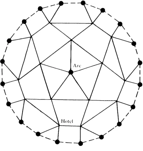
We turn now to the more complicated problem of a random walk on a two-dimensional array. In Figure 3 we illustrate such a walk. The large

Figure 3: ♣

dots represent boundary points; those markedE indicate escape routes and those marked P are police. We wish to find the probability p(x) that our walker, starting at an interior point x, will reach an escape route before he reaches a policeman. The walker moves fromx= (a, b) to each of the four neighboring points (a+ 1, b), (a−1, b), (a, b+ 1), (a, b−1) with probability ¹₄. If he reaches a boundary point, he remains at this point.

The corresponding voltage problem is shown in Figure 4. The boundary points P are grounded and points E are connected and fixed at one volt by a one-volt battery. We ask for the voltage v(x) at the interior points.

1.2.2 Harmonic functions in two dimensions

We now define harmonic functions for sets of lattice points in the plane (a lattice point is a point with integer coordinates). Let S = D∪B be a finite set of lattice points such that (a) D and B have no points in common, (b) every point of D has its four neighboring points in S, and (c) every point ofB has at least one of its four neighboring points

Figure 4: ♣

inD. We assume further that S hangs together in a nice way, namely, that for any two points P and Q in S, there is a sequence of points Pj in D such that P, P1, P2, . . . , Pn, Q forms a path from P to A. We call the points of D the interior points of S and the points of B the boundary points of S.

A function f defined on S is harmonic if, for points (a, b) in D, it has the averaging property

f(a, b) = f(a+ 1, b) +f(a−1, b) +f(a, b+ 1) +f(a, b−1)

4 .

Note that there is no restriction on the values of f at the boundary points.

We would like to prove that p(x) = v(x) as we did in the one- dimensional case. That p(x) is harmonic follows again by considering all four possible first steps; that v(x) is harmonic follows again by Kirchhoff’s Laws since the current coming into x= (a, b) is

v(a+ 1, b)−v(a, b)

R +v(a−1, b)−v(a, b)

R +v(a, b+ 1)−v(a, b)

R +v(a, b−1)−v(a, b)

R = 0.

Multiplying through by R and solving for v(a, b) gives

v(a, b) = v(a+ 1, b) +v(a−1, b) +v(a, b+ 1) +v(a, b−1)

4 .

Thus p(x) andv(x) are harmonic functions with the same boundary values. To show from this that they are the same, we must extend the Uniqueness Principle to two dimensions.

We first prove the Maximum Principle. IfM is the maximum value of f and if f(P) = M for P an interior point, then since f(P) is the average of the values of f at its neighbors, these values must all equal M also. By working our way due south, say, repeating this argument at every step, we eventually reach a boundary point Q for which we can conclude that f(Q) = M. Thus a harmonic function always attains its maximum (or minimum) on the boundary; this is the Maximum Principle. The proof of the Uniqueness Principle goes through as before since again the difference of two harmonic functions is harmonic.

The fair game argument, using the Martingale Stopping Theorem, holds equally well and again gives an alternative proof of the existence and uniqueness to the solution of the Dirichlet problem.

Exercise 1.2.1 Show that if f and g are harmonic functions so is h= a·f +b·g for constants a and b. This is called the superposition principle.

Exercise 1.2.2 LetB1, B2, . . . , Bnbe the boundary points for a region S. Let ej(a, b) be a function that is harmonic in S and has boundary value 1 atBj and 0 at the other boundary points. Show that if arbitrary boundary values v1, v2, . . . , vn are assigned, we can find the harmonic function v with these values from the solutions e1, e2, . . . , en.

1.2.3 The Monte Carlo solution

Finding the exact solution to a Dirichlet problem in two dimensions is not always a simple matter, so before taking on this problem, we will consider two methods for generating approximate solutions. In this section we will present a method using random walks. This method is known as a Monte Carlo method, since random walks are random, and gambling involves randomness, and there is a famous gambling casino in Monte Carlo. In Section 1.2.4, we will describe a much more effective method for finding approximate solutions, called the method of relaxations.

We have seen that the solution to the Dirichlet problem can be found by finding the value of a player’s final winning in the following game: Starting atxthe player carries out a random walk until reaching a boundary point. He is then paid an amountf(y) ifyis the boundary

point first reached. Thus to findf(x), we can start many random walks atx and find the average final winnings for these walks. By the law of averages (the law of large numbers in probability theory), the estimate that we obtain this way will approach the true expected final winning f(x).

Here are some estimates obtained this way by starting 10,000 ran- dom walks from each of the interior points and, for each x, estimating f(x) by the average winning of the random walkers who started at this point.

1 1

1.824 .785 1 1 .876 .503 .317 0

1 0 0

This method is a colorful way to solve the problem, but quite inef- ficient. We can use probability theory to estimate how inefficient it is.

We consider the case with boundary values I or 0 as in our example.

In this case, the expected final winning is just the probability that the walk ends up at a boundary point with value 1. For each point x, as- sume that we carry out n random walks; we regard each random walk to be an experiment and interpret the outcome of the ith experiment to be a “success” if the walker ends at a boundary point with a 1 and a “failure” otherwise. Let p = p(x) be the unknown probability for success for a walker starting at x and q = 1−p. How many walks should we carry out to get a reasonable estimate for p? We estimate p to be the fraction ¯p of the walkers that end at a 1.

We are in the position of a pollster who wishes to estimate the proportion p of people in the country who favor candidate A over B. The pollster chooses a random sample of n people and estimates p as the proportion ¯p of voters in his sample who favor A. (This is a gross oversimplification of what a pollster does, of course.) To estimate the number n required, we can use the central limit theorem. This theorem states that, if Sn, is the number of successes inn independent experiments, each having probability pfor success, then for any k >0

P −k < Sn−np

√npq < k

!

≈A(k),

where A(k) is the area under the normal curve between −k and k.

For k = 2 this area is approximately .95; what does this say about

¯

p=Sn/n? Doing a little rearranging, we see that P



−2< p¯−p

q_pq

n

<2



≈.95 or

P −2

√pq

n <p¯−p <2

√pq n

!

≈.95.

Since √pq≤ ¹2,

P − 1

√n <p¯−p < 1

√n

! >

≈.95.

Thus, if we choose ^√1_n =.01, orn = 10,000, there is a 95 percent chance that our estimate ¯p = Sn/n will not be off by more than .01. This is a large number for rather modest accuracy; in our example we carried out 10,000 walks from each point and this required about 5 seconds on the Dartmouth computer. We shall see later, when we obtain an exact solution, that we did obtain the accuracy predicted.

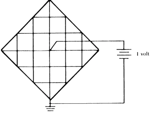
Exercise 1.2.3 You play a game in which you start a random walk at the center in the grid shown in Figure 5. When the walk reaches

Figure 5: ♣

the boundary, you receive a payment of +1 or −1 as indicated at the boundary points. You wish to simulate this game to see if it is a favorable game to play; how many simulations would you need to be reasonably certain of the value of this game to an accuracy of .01?

Carry out such a simulation and see if you feel that it is a favorable game.

1.2.4 The original Dirichlet problem; the method of relax- ations

The Dirichlet problem we have been studying is not the original Dirich- let problem, but a discrete version of it. The original Dirichlet problem concerns the distribution of temperature, say, in a continuous medium;

the following is a representative example.

Suppose we have a thin sheet of metal gotten by cutting out a small square from the center of a large square. The inner boundary is kept at temperature 0 and the outer boundary is kept at temperature 1 as indicated in Figure 6. The problem is to find the temperature at points in the rectangle’s interior. Ifu(x, y) is the temperature at (x, y), then u satisfies Laplace’s differential equation

uxx+uyy = 0.

A function that satisfies this differential equation is called harmonic. It has the property that the value u(x, y) is equal to the average of the values over any circle with center (x, y) lying inside the region. Thus to determine the temperature u(x, y), we must find a harmonic function defined in the rectangle that takes on the prescribed boundary values.

We have a problem entirely analogous to our discrete Dirichlet problem, but with continuous domain.

The method of relaxations was introduced as a way to get approx- imate solutions to the original Dirichlet problem. This method is ac- tually more closely connected to the discrete Dirichlet problem than to the continuous problem. Why? Because, faced with the continuous problem just described, no physicist will hesitate to replace it with an analogous discrete problem, approximating the continuous medium by an array of lattice points such as that depicted in Figure 7, and search- ing for a function that is harmonic in our discrete sense and that takes on the appropriate boundary values. It is this approximating discrete problem to which the method of relaxations applies.

Here’s how the method goes. Recall that we are looking for a func- tion that has specified boundary values, for which the value at any

Figure 6: ♣

Figure 7: ♣

interior point is the average of the values at its neighbors. Begin with any function having the specified boundary values, pick an interior point, and see what is happening there. In general, the value of the function at the point we are looking at will not be equal to the average of the values at its neighbors. So adjust the value of the function to be equal to the average of the values at its neighbors. Now run through the rest of the interior points, repeating this process. When you have adjusted the values at all of the interior points, the function that re- sults will not be harmonic, because most of the time after adjusting the value at a point to be the average value at its neighbors, we afterwards came along and adjusted the values at one or more of those neighbors, thus destroying the harmony. However, the function that results after running through all the interior points, if not harmonic, is more nearly harmonic than the function we started with; if we keep repeating this averaging process, running through all of the interior points again and again, the function will approximate more and more closely the solution to our Dirichlet problem.

We do not yet have the tools to prove that this method works for a general initial guess; this will have to wait until later (see Exercise 1.3.12). We will start with a special choice of initial values for which we can prove that the method works (see Exercise 1.2.5).

We start with all interior points 0 and keep the boundary points fixed.

1 1 1 0 0 1 1 0 0 0 0

1 0 0 After one iteration we have:

1 1

1 .547 .648 1 1 .75 .188 .047 0

1 0 0

Note that we go from left to right moving up each column replacing each value by the average of the four neighboring values. The compu- tations for this first iteration are

.75 = (1/4)(1 + 1 + 1 + 0) .1875 = (1/4)(.75 + 0 + 0 + 0) .5469 = (1/4)(.1875 + 1 + 1 + 0)

.0469 = (1/4)(.1875 + 0 + 0 + 0) .64844 = (1/4)(.0469 +.5769 + 1 + 1)

We have printed the results to three decimal places. We continue the iteration until we obtain the same results to three decimal places. This occurs at iterations 8 and 9. Here’s what we get:

1 1

1 .823 .787 1 1 .876 .506 .323 0

1 0 0

We see that we obtain the same result to three places after only nine iterations and this took only a fraction of a second of computing time.

We shall see that these results are correct to three place accuracy. Our Monte Carlo method took several seconds of computing time and did not even give three place accuracy.

The classical reference for the method of relaxations as a means of finding approximate solutions to continuous problems is Courant, Friedrichs, and Lewy [3]. For more information on the relationship between the original Dirichlet problem and the discrete analog, see Hersh and Griego [10].

Exercise 1.2.4 Apply the method of relaxations to the discrete prob- lem illustrated in Figure 7.

Exercise 1.2.5 Consider the method of relaxations started with an initial guess with the property that the value at each point is ≤ the average of the values at the neighbors of this point. Show that the successive values at a point u are monotone increasing with a limit f(u) and that these limits provide a solution to the Dirichlet problem.

1.2.5 Solution by solving linear equations

In this section we will show how to find an exact solution to a two- dimensional Dirichlet problem by solving a system of linear equations.

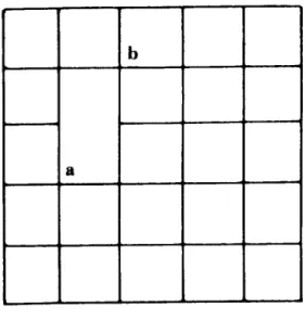
As usual, we will illustrate the method in the case of the example introduced in Section 1.2.1. This example is shown again in Figure 8; the interior points have been labelled a, b, c, d, and e. By our averaging property, we have

x_a= xb+xd+ 2 4

Figure 8: ♣ xb = xa+xc+ 2

4 xc = x_d+ 3

4 xd = xa+xc+xe

4 xe = xb+xd

4 .

We can rewrite these equations in matrix form as















1 −1/4 0 −1/4 0

−1/4 1 0 0 −1/4

0 0 1 −1/4 0

−1/4 0 −1/4 1 −1/4

0 −1/4 0 −1/4 1





























xa

x_b xc

xd

x_e















=















1/2 1/2 3/4 0 0















.

We can write this in symbols as

Ax=u.

Since we know there is a unique solution, A must have an inverse and x=A⁻¹u.

Carrying out this calculation we find

Calculated x=















.823 .787 .876 .506 .323















.

Here, for comparison, are the approximate solutions found earlier:

Monte Carlo x=















.824 .785 .876 .503 .317















.

Relaxed x=















.823 .787 .876 .506 .323















.

We see that our Monte Carlo approximations were fairly good in that no error of the simulation is greater than .01, and our relaxed approx- imations were very good indeed, in that the error does not show up at all.

Exercise 1.2.6 Consider a random walker on the graph of Figure 9.

Find the probability of reaching the point with a 1 before any of the points with 0’s for each starting point a, b, c, d.

Exercise 1.2.7 Solve the discrete Dirichlet problem for the graph shown in Figure 10. The interior points are a, b, c, d. (Hint: See Exercise 1.2.2.)

Exercise 1.2.8 Find the exact value, for each possible starting point, for the game described in Exercise 1.2.3. Is the game favorable starting in the center?

1.2.6 Solution by the method of Markov chains

In this section, we describe how the Dirichlet problem can be solved by the method of Markov chains. This method may be viewed as a more sophisticated version of the method of linear equations.

Figure 9: ♣

Figure 10: ♣

A finite Markov chain is a special type of chance process that may be described informally as follows: we have a set S = {s₁, s₂, . . . , s_r} ofstates and a chance process that moves around through these states.

When the process is in state si, it moves with probability Pij to the state s_j. The transition probabilities P_ij are represented by an r-by-r matrix P called the transition matrix. To specify the chance process completely we must give, in addition to the transition matrix, a method for starting the process. We do this by specifying a specific state in which the process starts.

According to Kemeny, Snell, and Thompson [15], in the Land of Oz, there are three kinds of weather: rain, nice, and snow. There are never two nice days in a row. When it rains or snows, half the time it is the same the next day. If the weather changes, the chances are equal for a change to each of the other two types of weather. We regard the weather in the Land of Oz as a Markov chain with transition matrix:

P=







R N S

R 1/2 1/4 1/4

N 1/2 0 1/2

S 1/4 1/4 1/2





.

When we start in a particular state, it is natural to ask for the probability that the process is in each of the possible states after a specific number of steps. In the study of Markov chains, it is shown that this information is provided by the powers of the transition matrix.

Specifically, if Pⁿ is the matrix P raised to the nth power, the entries P_ijⁿ represent the probability that the chain, started in state s_i, will, after n steps, be in state sj. For example, the fourth power of the transition matrix P for the weather in the Land of Oz is

P⁴ =







R N S

R .402 .199 .398 N .398 .203 .398 S .398 .199 .402





.

Thus, if it is raining today in the Land of Oz, the probability that the weather will be nice four days from now is .199. Note that the probability of a particular type of weather four days from today is es- sentially independent of the type of weather today. This Markov chain is an example of a type of chain called a regular chain. A Markov chain is a regular chain if some power of the transition matrix has no zeros.

In the study of regular Markov chains, it is shown that the probability

of being in a state after a large number of steps is independent of the starting state.

As a second example, we consider a random walk in one dimension.

Let us assume that the walk is stopped when it reaches either state 0 or 4. (We could use 5 instead of 4, as before, but we want to keep the matrices small.) We can regard this random walk as a Markov chain with states 0, 1, 2, 3, 4 and transition matrix given by

P=

















0 1 2 3 4

0 1 0 0 0 0

1 1/2 0 1/2 0 0

2 0 1/2 0 1/2 0

3 0 0 1/2 0 1/2

4 0 0 0 0 1

















.

The states 0 and 4 are traps or absorbing states. These are states that, once entered, cannot be left. A Markov chain is called absorbing if it has at least one absorbing state and if, from any state, it is possible (not necessarily in one step) to reach at least one absorbing state. Our Markov chain has this property and so is an absorbing Markov chain.

The states of an absorbing chain that are not traps are called non- absorbing.

When an absorbing Markov chain is started in a non-absorbing state, it will eventually end up in an absorbing state. For non-absorbing state s_i and absorbing state s_j, we denote by B_ij the probability that the chain starting in si will end up in state sj. We denote by B the matrix with entries Bij. This matrix will have as many rows as non- absorbing states and as many columns as there are absorbing states.

For our random walk example, the entriesBx,4 will give the probability that our random walker, starting at x, will reach 4 before reaching 0.

Thus, if we can find the matrixB by Markov chain techniques, we will have a way to solve the Dirichlet problem.

We shall show, in fact, that the Dirichlet problem has a natural generalization in the context of absorbing Markov chains and can be solved by Markov chain methods.

Assume now thatPis an absorbing Markov chain and that there are u absorbing states and v non-absorbing states. We reorder the states so that the absorbing states come first and the non-absorbing states come last. Then our transition matrix has the canonical form:

P=

I 0 R Q

.

Here I is a u-by-u identity matrix; 0 is a matrix of dimension u-by-v with all entries 0.

For our random walk example this canonical form is:

















0 4 1 2 3

0 1 0 0 0 0

4 0 1 0 0 0

1 1/2 0 0 1/2 0

2 0 0 1/2 0 1/2

3 0 1/2 0 1/2 0

















.

The matrix N = (I−Q)⁻¹ is called the fundamental matrix for the absorbing chainP. (Note that I here is a v-by-v identity matrix!) The entriesNijof this matrix have the following probabilistic interpretation:

Nij is the expected number of times that the chain will be in state sj

before absorption when it is started in si. (To see why this is true, think of how (I−Q)⁻¹ would look if it were written as a geometric series.) Let 1 be a column vector of all 1’s. Then the vector t = NI gives the expected number of steps before absorption for each starting state.

The absorption probabilities B are obtained fromN by the matrix formula

B = (I−Q)⁻¹R.

This simply says that to get the probability of ending up at a given absorbing state, we add up the probabilities of going there from all the non-absorbing states, weighted by the number of times we expect to be in those (non-absorbing) states.

For our random walk example Q=







0 ¹₂ 0

1

2 0 ¹₂ 0 ¹₂ 0







I−Q=







1 −¹₂ 0

−¹₂ 1 −¹₂ 0 −¹2 1







N= (I−Q)⁻¹ =







1 2 3

1 ³₂ 1 ¹₂

2 1 2 1

3 ¹₂ 1 ³₂







t=N1=







3

2 1 ¹₂

1 2 1

1

2 1 ³₂













1 1 1





=







3 4 3







B =NR=







3

2 1 ¹₂

1 2 1

1

2 1 ³₂













1

2 0

0 0 0 ¹₂





=







0 4 1 ³₄ ¹₄ 2 ¹₂ ¹₂ 3 ¹₄ ³₄





.

Thus, starting in state 3, the probability is 3/4 of reaching 4 before 0; this is in agreement with our previous results. From t we see that the expected duration of the game, when we start in state 2, is 4.

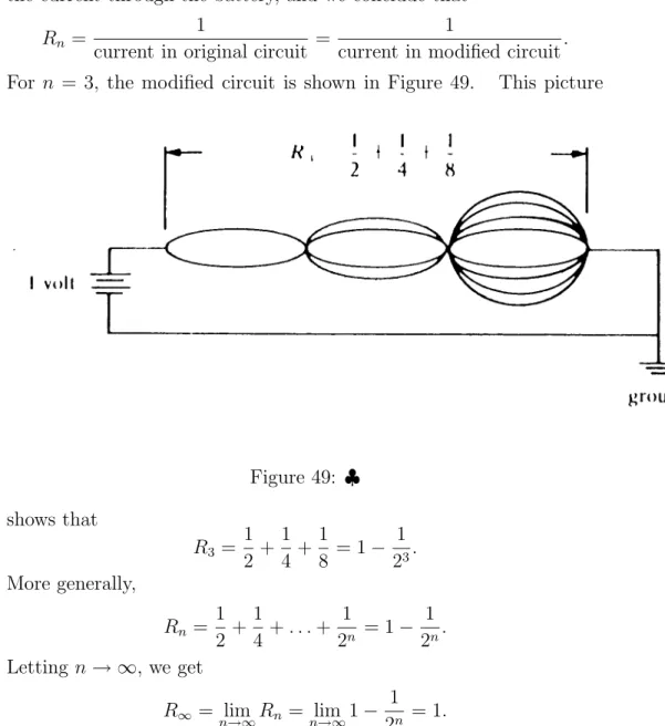
For an absorbing chain P, thenth power Pⁿof the transition prob- abilities will approach a matrix P^∞ of the form

P^∞=

I 0 B 0

.

We now give our Markov chain version of the Dirichlet problem. We interpret the absorbing states as boundary states and the non-absorbing states as interior states. LetB be the set of boundary states andDthe set of interior states. Let f be a function with domain the state space of a Markov chain Psuch that for i inD

f(i) = ^X

j

Pijf(j).

Then f is a harmonic function for P. Now f again has an averaging property and extends our previous definition. If we represent f as a column vector f, f is harmonic if and only if

Pf =f. This implies that

P²f =P·Pf =Pf =f and in general

Pⁿf =f. Let us write the vector f as

f =

fB

fD

where fB represents the values of f on the boundary and fD values on the interior. Then we have

fB

fD

=

I 0 B Q

fB

fD

and

f_D =Bf_B.

We again see that the values of a harmonic function are determined by the values of the function at the boundary points.

Since the entries Bij of B represent the probability, starting in i, that the process ends at j, our last equation states that if you play a game in which your fortune is f_j when you are in state j, then your expected final fortune is equal to your initial fortune; that is, fairness is preserved. As remarked above, from Markov chain theory B =NR where N= (I−Q)⁻¹. Thus

fD = (I−Q)⁻¹RfB.

(To make the correspondence between this solution and the solution of Section 1.2.5, putA =I−Q and u=Rf_B.)

A general discussion of absorbing Markov chains may be found in Kemeny, Snell, and Thompson [15].

Exercise 1.2.9 Consider the game played on the grid in Figure 11.

You start at an interior point and move randomly until a boundary

Figure 11: ♣

point is reached and obtain the payment indicated at this point. Using Markov chain methods find, for each starting state, the expected value of the game. Find also the expected duration of the game.

1.3 Random walks on more general networks

1.3.1 General resistor networks and reversible Markov chains Our networks so far have been very special networks with unit resistors.

We will now introduce general resistor networks, and consider what it means to carry out a random walk on such a network.

Agraph is a finite collection ofpoints (also calledvertices ornodes) with certain pairs of points connected by edges (also called branches).

The graph is connected if it is possible to go between any two points by moving along the edges. (See Figure 12.)

Figure 12: ♣

We assume that Gis a connected graph and assign to each edgexy a resistance Rxy; an example is shown in Figure 13. Theconductance of an edge xyis Cxy = 1/Rxy; conductances for our example are shown in Figure 14.

We define arandom walk onGto be a Markov chain with transition matrix P given by

Pxy = Cxy

Cx

with Cx = ^P_yCxy. For our example, Ca = 2, Cb = 3, Cc = 4, and Cd = 5, and the transition matrix Pfor the associated random walk is











a b c d a 0 0 ¹₂ ¹₂ b 0 0 ¹₃ ²₃ c ¹₄ ¹₄ 0 ¹₂ d ¹₅ ²₅ ²₅ 0











Figure 13: ♣

Figure 14: ♣

Figure 15: ♣

Its graphical representation is shown in Figure 15.

Since the graph is connected, it is possible for the walker to go between any two states. A Markov chain with this property is called an ergodic Markov chain. Regular chains, which were introduced in Section 1.2.6, are always ergodic, but ergodic chains are not always regular (see Exercise 1.3.1).

For an ergodic chain, there is a unique probability vector w that is a fixed vector for P, i.e.,wP=w. The component wj of wrepresents the proportion of times, in the long run, that the walker will be in state j. For random walks determined by electric networks, the fixed vector is given bywj =Cj/C, whereC =^P_xCx. (You are asked to prove this in Exercise 1.3.2.) For our example Ca = 2, Cb = 3, Cc = 4, Cd = 5, and C = 14. Thus w= (2/14,3/14,4/14,5/14). We can check that w is a fixed vector by noting that

(₁₄² ₁₄³ ₁₄⁴ ₁₄⁵ )











0 0 ¹₂ ¹₂ 0 0 ¹₃ ²₃

1 4

1

4 0 ¹₂

1 5

2 5

2

5 0











= (₁₄² ₁₄³ ₁₄⁴ ₁₄⁵ ).

In addition to being ergodic, Markov chains associated with net- works have another property called reversibility. An ergodic chain is said to be reversible if wxPxy =wyPyx for allx, y. That this is true for our network chains follows from the fact that

CxPxy =Cx

C_xy Cx

=Cxy =Cyx =Cy

C_yx Cy

=CyPyx.

Thus, dividing the first and last term by C, we have wxPxy =wyPyx. To see the meaning of reversibility, we start our Markov chain with initial probabilities w (in equilibrium) and observe a few states, for example

a c b d.

The probability that this sequence occurs is w_aP_acP_cbP_bd= 2

14· 1 2 ·1

4 · 2 3 = 1

84. The probability that the reversed sequence

d b c a occurs is

wdPdbPbcPca = 5 14· 2

5 ·1 3 · 1

4 = 1 84.

Thus the two sequences have the same probability of occurring.

In general, when a reversible Markov chain is started in equilibrium, probabilities for sequences in the correct order of time are the same as those with time reversed. Thus, from data, we would never be able to tell the direction of time.

If P is any reversible ergodic chain, then P is the transition ma- trix for a random walk on an electric network; we have only to define Cxy = wxPxy. Note, however, if Pxx 6= 0 the resulting network will need a conductance from xtox(see Exercise 1.3.4). Thus reversibility characterizes those ergodic chains that arise from electrical networks.

This has to do with the fact that the physical laws that govern the behavior of steady electric currents are invariant under time-reversal (see Onsager [25]).

When all the conductances of a network are equal, the associated random walk on the graphGof the network has the property that, from each point, there is an equal probability of moving to each of the points connected to this point by an edge. We shall refer to this random walk

assimple random walk onG. Most of the examples we have considered so far are simple random walks. Our first example of a random walk on Madison Avenue corresponds to simple random walk on the graph with points 0,1,2, . . . , N and edges the streets connecting these points.

Our walks on two dimensional graphs were also simple random walks.

Exercise 1.3.1 Give an example of an ergodic Markov chain that is not regular. (Hint: a chain with two states will do.)

Exercise 1.3.2 Show that, if P is the transition matrix for a random walk determined by an electric network, then the fixed vectorwis given by wx = ^C_C^x where Cx =^P_yCxy and C =^P_xCx.

Exercise 1.3.3 Show that, ifPis a reversible Markov chain anda, b, c are any three states, then the probability, starting at a, of the cycle abca is the same as the probability of the reversed cycle acba. That is P_abP_bcP_ca = P_acP_cbP_ba. Show, more generally, that the probability of going around any cycle in the two different directions is the same.

(Conversely, if this cyclic condition is satisfied, the process is reversible.

For a proof, see Kelly [13].)

Exercise 1.3.4 Assume thatPis a reversible Markov chain withPxx = 0 for all x. Define an electric network by Cxy =wxPxy. Show that the Markov chain associated with this circuit is P. Show that we can allow Pxx >0 by allowing a conductance from x tox.

Exercise 1.3.5 For the Ehrenfest urn model, there are two urns that together contain N balls. Each second, one of the N balls is chosen at random and moved to the other urn. We form a Markov chain with states the number of balls in one of the urns. ForN = 4, the resulting transition matrix is

P=

















0 1 2 3 4

0 0 1 0 0 0

1 ¹₄ 0 ³₄ 0 0 2 0 ¹₂ 0 ¹₂ 0 3 0 0 ³₄ 0 ¹₄

4 0 0 0 1 0

















.

Show that the fixed vectorwis the binomial distributionw= (₁₆¹,₁₆⁴,₁₆⁶ ,₁₆⁴ ,₁₆¹).

Determine the electric network associated with this chain.

1.3.2 Voltages for general networks; probabilistic interpreta- tion

We assume that we have a network of resistors assigned to the edges of a connected graph. We choose two points a and b and put a one-volt battery across these points establishing a voltage va = 1 and vb = 0, as illustrated in Figure 16. We are interested in finding the volt-

Figure 16: ♣

ages vx and the currents ixy in the circuit and in giving a probabilistic interpretation to these quantities.

We begin with the probabilistic interpretation of voltage. It will come as no surprise that we will interpret the voltage as a hitting prob- ability, observing that both functions are harmonic and that they have the same boundary values.

By Ohm’s Law, the currents through the resistors are determined by the voltages by

ixy = vx−vy

Rxy

= (Vx−vy)Cxy.

Note that ixy =−iyx. Kirchhoff’s Current Law requires that the total current flowing into any point other thanaorbis 0. That is, forx6=a, b

X

y

ixy = 0.

This will be true if

X

y

(v_x−v_y)C_xy = 0 or

vx

X

y

Cxy =^X

y

Cxyvy.

Thus Kirchhoff’s Current Law requires that our voltages have the prop- erty that

vx =^X

y

Cxy

Cx

vy =^X

y

Pxyvy

for x 6= a, b. This means that the voltage vx is harmonic at all points x6=a, b.

Lethxbe the probability, starting atx, that stateais reached before b. Then hx is also harmonic at all points x6=a, b. Furthermore

va=ha= 1 and

vb =hb = 0.

Thus if we modify P by making a and b absorbing states, we obtain an absorbing Markov chain P¯ and v and h are both solutions to the Dirichlet problem for the Markov chain with the same boundary values.

Hence v =h.

For our example, the transition probabilities ¯Pxy are shown in Figure 17. The function vx is harmonic for ¯P with boundary values va = 1, v_b = 0.

To sum up, we have the following:

Intrepretation of Voltage. When a unit voltage is applied be- tweenaand b, making v_a = 1 andv_b = 0, the voltagev_x at any point x represents the probability that a walker starting from x will return to a before reaching b.

In this probabilistic interpretation of voltage, we have assumed a unit voltage, but we could have assumed an arbitrary voltage va be- tween a and b. Then the hitting probability hx would be replaced by an expected value in a game where the player starts at x and is paid va if a is reached before b and 0 otherwise.

Let’s use this interpretation of voltage to find the voltages for our example. Referring back to Figure 17, we see that

va = 1

Figure 17: ♣ vb = 0 vc= 1

4 +1 2vd

vd = 1 5 + 2

5vc.

Solving these equations yields vc = ₁₆⁷ and vd = ³₈. From these voltages we obtain the current i_xy. For example i_cd = (₁₆⁷ − ³₈)·2 = ¹₈. The resulting voltages and currents are shown in Figure 18. The voltage at c is ₁₆⁷ and so this is also the probability, starting at c, of reaching a beforeb.

1.3.3 Probabilistic interpretation of current

We turn now to the probabilistic interpretation of current. This in- terpretation is found by taking a naive view of the process of electri- cal conduction: We imagine that positively charged particles enter the network at point a and wander around from point to point until they finally arrive at point b, where they leave the network. (It would be more realistic to imagine negatively charged particles entering at band

Figure 18: ♣

leaving at a, but realism is not what we’re after.) To determine the currenti_xy along the branch fromxtoy, we consider that in the course of its peregrinations the point may pass once or several times along the branch fromx toy, and in the opposite direction fromytox. We may now hypothesize that the currenti_xy is proportional to the expected net number of movements along the edge from x to y, where movements from y back to x are counted as negative. This hypothesis is correct, as we will now show.

The walker begins at a and walks until he reaches b; note that if he returns to a before reaching b, he keeps on going. Let ux be the expected number of visits to state x before reaching b. Then ub = 0 and, for x6=a, b,

ux =^X

y

uyPyx.

This last equation is true because, for x 6= a, b, every entrance to x must come from some y.

We have seen that CxPxy =CyPyx; thus ux =^X

y

uy

PxyCx

Cy

or ux

Cx

=^X

y

Pxy

uy

Cy

.

This means that vx = ux/Cx is harmonic for x 6= a, b. We have also vb = 0 and va =ua/Ca. This implies that vx is the voltage at x when we put a battery from a tob that establishes a voltage ua/Ca ata and voltage 0 at b. (We remark that the expression vx = ux/Cx may be understood physically by viewing ux as charge and Cx as capacitance;

see Kelly [13] for more about this.)

We are interested in the current that flows from x toy. This is ixy = (vx−vy)Cxy = ux

Cx − uy

Cy

!

Cxy = uxCxy

Cx −uyCyx

Cy

=uxPxy−uyPyx. Now u_xP_xy is the expected number of times our walker will go from x to y and uyPyx is the expected number of times he will go from y to x. Thus the current ixy is the expected value for the net number of times the walker passes along the edge from x toy. Note that for any particular walk this net value will be an integer, but the expected value will not.