Efficient semiclassical approach for time delays

This content has been downloaded from IOPscience. Please scroll down to see the full text.

Download details:

IP Address: 132.199.144.70

This content was downloaded on 27/02/2015 at 10:35

Please note that terms and conditions apply.

Efficient semiclassical approach for time delays

View the table of contents for this issue, or go to the journal homepage for more 2014 New J. Phys. 16 123018

(http://iopscience.iop.org/1367-2630/16/12/123018)

Jack Kuipers¹, Dmitry V Savin²and Martin Sieber³

1Institut für Theoretische Physik, Universität Regensburg, D-93040 Regensburg, Germany

2Department of Mathematics, Brunel University London, Uxbridge, UB8 3PH, UK

3School of Mathematics, University of Bristol, Bristol, BS8 1TW, UK E-mail:jack.kuipers@ur.de

Received 10 September 2014, revised 27 October 2014 Accepted for publication 29 October 2014

Published 8 December 2014

New Journal of Physics16(2014) 123018 doi:10.1088/1367-2630/16/12/123018

Abstract

The Wigner time delay, defined by the energy derivative of the total scattering phase shift, is an important spectral measure of an open quantum system char- acterizing the duration of the scattering event. It is proportional to the trace of the Wigner–Smith matrix Q that also encodes other time-delay characteristics. For chaotic cavities, these quantities exhibit universal fluctuations that are com- monly described within random matrix theory. Here, we develop a new semi- classical approach to the time-delay matrix which is formulated in terms of the classical trajectories that connect the exterior and interior regions of the system.

This approach is superior to previous treatments because it avoids the energy derivative. We demonstrate the methodʼs efficiency by going beyond previous work in establishing the universality of time-delay statistics for chaotic cavities with perfectly connected leads. In particular, the moment generating function of the proper time-delays (eigenvalues of Q) is found semiclassically for the first five orders in the inverse number of scattering channels for systems with and without time-reversal symmetry. We also show the equivalence of random matrix and semiclassical results for the second moments and for the variance of the Wigner time delay at any channel number.

Keywords: semiclassical approach, random matrix theory, Wigner time delay

Content from this work may be used under the terms of theCreative Commons Attribution 3.0 licence.

Any further distribution of this work must maintain attribution to the author(s) and the title of the work, journal citation and DOI.

1. Introduction

The concept of time delay plays an important and special role in quantum collision theory. It was first introduced by Eisenbud and Wigner [1, 2] in the context of elastic scattering, who related the time during which a monochromatic wave packet is delayed in the interaction region to the energy derivative of the scattering phase shift. Later on Smith [3] extended the concept to the case of inelastic scattering with many channels and introduced the time-delay (or Wigner– Smith) matrix

⎜ ⎟ ⎜ ⎟

⎡

⎣⎢ ⎛

⎝ ⎞

⎠ ⎛

⎝ ⎞

⎠

⎤

⎦⎥

ϵ

ϵ ϵ

= − = − − +

ϵ=

 

Q E S E S E

E S E S E

( ) i ( )d ( )

d i d

d 2 2 , (1)

† †

0

whereS(E) is the scattering matrix at energyEwhose dimension is given by the number of open channels, M. For an energy and flux conserving scatterer (i.e. involving no absorption or dissipation), the S-matrix is unitary and Q is a Hermitian matrix, which is manifest from the second representation in (1). The real characteristics of Q (e.g. its diagonal elements and eigenvalues) provide us with various time-delay related observables [3]. Taking the trace, one arrives at the simple weighted-mean measure of the collision duration [4–7]

τ ≡ = − 

E M Q E

M E S E

( ) 1

Tr ( ) i d

d ln det ( ). (2)

W

This expression defines the Wigner time delay in multi-channel scattering. Further and more subtle discussions of the physical concepts of time delays and their applications to regular and chaotic scattering can be found in recent reviews [7–9].

As is clear from the definition, the dominant contributions to τW come from the regions where the total scattering phase shift exhibits a sharp energy dependence. Away from the channel thresholds, this occurs in the vicinity of resonances that correspond to the meta-stable (decaying) states formed at the intermediate stage of the scattering event. Such resonances can be analytically viewed as the complex poles _n = E_n − ⁱΓ_n

2 of the S-matrix in the complex energy plane, withE_nandΓnbeing the position and width of thenth resonance, respectively. In the resonance approximation, neglecting the constant background connected to potential scattering and direct reactions, these poles are the only singularities ofS. In view of the unitarity condition, their complex conjugates n* serve as the S-matrix zeros, thus implying



= ∏ ⁻

S −

det _n ^E

E

n n

*. This results in the important connection [4, 6]

∑

τ Γ

Γ

=

− +



( )

E M

E E

( ) 1

4

, (3)

n

n

n n

W 2 2

between the Wigner time delay and the resonance spectrum of the intermediate open system.

This expression is valid at arbitrary degree of the resonance overlap and thus the Winger time delay (2) can also be treated as the density of states of the open system, see [10,11] for relevant discussion. In particular, the spectral average of τ_W over a narrow energy window is τ¯W= 2π ρ¯ M, where ρ¯ is the mean density around E. The latter in turn determines the fundamental timescale in quantum systems, the Heisenberg time TH = 2π ρ¯, so that τ¯_W= T M_H .

In many experimental situations, the intermediate system is characterized by very complicated internal motion, with representative examples being microwave cavities [12],

quantum dots [13] and compound nuclei [14]. As a result, the time delay (as well as other scattering observables) reveals strongfluctuations around its mean value that need to be treated statistically. There are two main approaches to describe suchfluctuations: random matrix theory (RMT) [15] and the semiclassical method [16].

The general RMT approach to the time delay, mostly developed in [6,7,17], is based on a representation of the Wigner–Smith matrix in terms of the effective non-Hermitian Hamiltonian

eff of the open system. The complex resonancesn are then given by the eigenvalues of the Hamiltonian [18]. The Hermitian part ofeff describes the internal Hamiltonian with a discrete spectrum and chaotic dynamics. It can therefore be modelled by a randomN × N matrix drawn from the Gaussian orthogonal or unitary ensemble, depending on the presence or absence of time-reversal symmetry (TRS), respectively [15]. The anti-Hermitian part originates from coupling between theNinternal andMchannels states and has a specific algebraic structure due to the unitarity constraint [18]. The statistical averaging can then be performed by making use of the powerful supersymmetry technique, mapping the problem to a nonlinear supersymmetric σ-model of zero-dimensional field theory [19]. In the asymptotic limit N → ∞, the obtained results are universal in the sense that local fluctuations on the scale of mean level spacing

ρ ∼ N⁻

1 ¯ ¹ become model-independent provided that the appropriate natural units have been used [20]. The only parameters are then the number Mof open channels and their strength of coupling to the continuum. The later is quantified by the average‘optical’S-matrix, withS = 0 (orS → 1) being the limiting case of a perfectly open (or almost closed) system.

The exact universal results were initially obtained for the autocorrelation function of the Wigner time delay, first for orthogonal [6] and unitary symmetry [7], and then for the whole crossover of partly broken TRS [21]. Along these lines, exact formulae were also derived for the distribution function of thepartialtime-delays [7, 21] (defined by the energy derivatives of theS-matrix eigenphases and related to the diagonal elements ofQ [22]) as well as that of the propertime-delays (given by the eigenvalues ofQ) [17, 23]. The developed method is actually flexible enough to also include the effects of finite absorption [23, 24] and disorder [24, 25].

The most recent overview of the relevant results can be found in [26].

Further progress is possible in the particular case of perfect coupling, when Sis uniformly distributed in Dysonʼs circular ensemble of the appropriate symmetry [27]. Brouweret al[28]

exploited the invariance properties of the energy-dependentS-matrix in this case to derive the distribution of the whole time-delay matrix, generalizing the earlier one-channel result [29] to arbitraryM. The joint distribution function of its eigenvalues, i.e. the proper time-delays, turned out to be determined by the Laguerre ensemble from RMT [28]. This provided a route to apply orthogonal polynomials to compute marginal distributions [30] and various moments [31–34]

or use a Coulomb gas method to study the total density [35]. Very recently, Mezzadri and Simm [36] applied the integrable theory of certain matrix integrals to the problem and developed an efficient method for computing cumulants of arbitrary order. In particular, the variance of the Wigner time delay was found in the simple form,

τ

τ τ τ

≡ − = β

+ −

M M

var( ) 1

¯ ( ¯ ) 4

( 1)( 2), (4)

W

W2 W W 2

where 〈⋯〉 stands for a statistical average and β = 1 (β = 2) indicates orthogonal (unitary) symmetry. This expression agrees with earlier results obtained at arbitrary coupling in [6, 7].

We note, however, that the results for the distribution of Wigner time delay are still rather

limited, with explicit expressions being available only at M = 1, 2 [22, 37] or in the limit of

≫

M 1[35].

Taking a semiclassical approach, an early expression for the Wigner time delay was derived through the connection to the density of states mentioned above. Thefluctuating part of this quantity can be expressed, like Gutzwillerʼs trace formula for closed systems [16,38], as a sum over periodic orbits,

∑



τ − τ ≈ ^

M A

¯ 2

Re e , (5)

p m

p m m

W W

,

, ^p

i

but now only involving those orbits trapped inside the scattering system [39]. The trapped primitive orbitsp and their repetitions minvolve their actionsp and stability amplitudes Ap m,

which in turn depend on the period, monodromy matrix and Maslov index of the orbits. Since the dependence on the energy (and other parameters) is then encoded in the sum over the periodic orbits, this can be used to calculate correlation functions [40, 41], in particular, the time-delay variance is expressed as

∑

 

τ ≈

′

′ 

(

− ′

)

T A A

var( ) 2

Re e . (6)

p p p p W

H 2

,

* i p p

When taking the semiclassical limit →0, the rapid oscillations in the phase induced will be washed out by the overall spectral averaging unless there are systematic correlations between periodic orbits with action difference|p − p′|≲ . The repetitions have been ignored in (6) since they are exponentially smaller than them = 1 term. The semiclassical treatment of sums like in (6) then involves identifying and evaluating correlated pairs of orbits with a small action difference. The simplest pair is to set p = ′p, known as the diagonal approximation [42], which can be evaluated using the open system version [43] of the Hannay–Ozorio de Almeida sum rule [44]

∫

∑

≈ ^μ = μ

∞ −

A te dt 1

. (7)

p

p 2 t

0 2

Here the exponential weighting corresponds to the expected number of periodic orbits of the closed system which survive up to a timet, withμ = M TH being the classical escape rate (see, however, the discussion in [6, 45, 46]). With TRS, one can also pair an orbit with its time reverse and obtain a further factor of 2, or

τ = β +

(

⁻

)

M O M

var( ) 4

, (8)

W 2

3

thus reproducing (4) to leading order. This is not surprising, of course, as the quasiclassical limit in the RMT treatment corresponds to the asymptotic case of M ≫ 1 [5, 47]. The quantum effects are encoded in the higher order terms of the1 M expansion, being in general responsible for slowing down the decay law in chaotic systems from the purely exponential one [45]. It is now well understood that the higher order terms can be obtained semiclassically through a systematic expansion of correlated periodic pairs which was first derived for the spectral statistics of closed systems [48–50]. The extension to open systems and the time delay was then developed in [51], providing the terms up to M⁻⁸ in full agreement with the RMT result.

Further calculations along those lines become too involved because of the quickly growing

complexity of relevant combinatorics. One possibility to overcome such difficulties might be in doing the semiclassical approximation at the level of the generating functions [52] used to derive the correspondingσ-model of RMT [6,7], the idea that has already proven to be success in establishing the full equivalence with RMT for the closed systems [53]. However, we will exploit another route here.

An alternative starting point relies on the van Vleck approximation of the propagator that gives the semiclassical approximation for the scattering matrix elements [54–57] in terms of trajectories that connect the corresponding (say, input iand output o) channels

∑



≈

γ

γ

→

 γ

S T1 A

˜ e . (9)

oi

i o

H ( )

i

The scattering trajectories now have different stability amplitudes A˜γ which do not explicitly depend on the durationT_γ of the trajectories but still include a phase factor. Taking the energy derivative and noting that ∂_γ ∂E = T_γ, one obtains the approximation for the Wigner time delay [46]

∑ ∑

 

τ ≈

γ γ

γ γ γ

= ′ →

′ _

(

_γ− _γ′

)

MT1 T A A

˜ ˜ e , (10)

i o M

i o W

H , 1 , ( )

* ⁱ

where we have assumed that the amplitudes vary much more slowly than the phase. The diagonal approximationγ = ′γ can again be evaluated with a sum rule [58]

∫

∑ ∑

τ ≈ ≈ = μ

γ

γ γ μ

= →

∞ −

MT T A M

T t t

¯ 1 ˜ e d 1

, (11)

i o M

i o W t

H , 1 ( )

2

H 0

which directly gives the average time delay.

In the presence of TRS one can also partner a scattering trajectory with its time reverse if they start and end in the same channel. However there are further correlated pairs of trajectories, both with and without TRS. They can be related to correlated pairs of periodic orbits by formally cutting the periodic orbits open and deforming them into scattering trajectories [58–60]. It is worth stressing that the second form of the time-delay matrix in (1) turns out to be particularly useful for the semiclassical treatment. One can show in this way [61] that all further contributions to the average time delay cancel leaving only the diagonal terms intact. Furthermore, one can also derive (5) semiclassically from (10) by recreating the sum over periodic orbits in (5) from correlations of scattering trajectories that approach the trapped periodic orbits and follow them for many repetitions. This provides a duality between the two approaches and allows access to a range of statistics beyond the average time delay [61]. For example, the moments of the proper time-delays can be found to leading order in M⁻¹ by using energy-dependent correlators of the S-matrix elements and performing a semiclassical expansion for the later [62]. The next two orders can similarly be obtained using a recursive graphical representation of the semiclassical diagrams of correlated trajectories [63], showing an agreement with RMT [32], though the energy dependence, which is later differentiated out and removed as in (1), complicates the treatment drastically.

In this paper, we derive yet another semiclassical approximation to the time delay which avoids using such an energy differentiation in the first place and significantly

simplifies the semiclassical calculations. It builds upon the resonant representation [64] of the matrix elements Qcc′= b bc† c′

as the overlap of the internal parts b of the scattering wave functions in the incident channels c and c′. We note that with such a factorized form, calculations of the moments of the Wigner time delay have some resemblance with those of the conductance and shot noise in the Landauer–Büttiker formalism of quantum transport [65]. The statistics of the latter in chaotic cavities is determined by the Jacobi ensembles of RMT [27], the exact expressions for their first two cumulants being derived in [66].

Transport moments of arbitrary order can be obtained most efficiently by exploiting the connection with the Selberg integral [66, 67], see further developments in [68–71] as well as [31, 32, 36, 72–76] for other RMT studies on transport statistics. These results agreed with those from the semiclassical approach to quantum transport problems, as originally shown for the first two transport moments in [59, 60] and then generalized to an inverse channel expansion of all higher moments in [63, 77]. Here, we provide for the first time a similar semiclassical justification of the Laguerre ensembles of RMT. In particular, we derive the exact expression (4) for the variance of Wigner time delay semiclassically at any M both for unitary and orthogonal symmetry (along with the other second moments of time- delays). We also extend previous work [62, 63] on establishing the universality for the moment generating functions.

In the next section, we formulate our starting point and develop a semiclassical approximation to the internal partsb_cand establish diagrammatic sum rules. This representation is then applied in section 3 to derive the second moments of time-delays at arbitrary M.

Section 4deals with the moment generating function of the proper time-delays and works out the algorithmic approach for thefirstfive terms in a1M-expansion. Section5summarizes our findings. Finally, we provide several appendices with more technical details of our calculations, including sums for systems with TRS and a comparison to previous approaches, which we believe may be helpful for further development and applications of the method.

2. Resonance scattering approach

In the general scattering formalism, the resonance part of the scattering matrix can be represented in terms of the effective non-Hermitian Hamiltonian as follows [18, 19]:

 

= −

− = −

S V

E V H VV

1 i 1

, i

2 . (12)

†

eff

eff †

Here, the Hermitian N × N matrix H corresponds to the Hamiltonian of the closed system, whereas the rectangularN ×M matrixVconsists of the decay amplitudes that coupleNdiscrete energy levels to M decay channels. These amplitudes are commonly treated as energy- independent quantities, which can be justified by considering resonance phenomena away from the open channel thresholds. Substituting (12) into (1), one can readilyfind the representation of the Wigner–Smith matrix [64],

 

=

− − ≡

 

( )

Q V

E 1 E 1 V b b

, (13)

†

eff

† eff

†

in terms of theN ×Mmatrixb = (E − eff)⁻1V. In such an approach, the energy dependence enters only via the resolvent(E − _eff)⁻¹ that describes the propagation in the open system

governed byeff. TheN-component vectorb_c(i.e. thecth column ofb) can therefore be treated [64] as the intrinsic part of the scattering wave function initiated in the channel cat energy E.

The diagonal elementsq_c = Q_ccare then given by the norm ofb_c, providing the interpretation as the average time delay of a wave packet in a given channel [3]. Taking the sum over the diagonal elements, wefind that the Wigner time delay is given by the total norm of the internal parts

∑

τ = = ∥ ∥

=

M1 q q  b

, . (14)

c M

c c c

W

1

2

This norm is also known as the dwell time, thus the two time characteristics coincide in the resonance approximation considered.

The factorized representation (13) already proved [17, 23] to be successful for deriving the exact (RMT) distributions of the proper time-delays (the eigenvalues of Q) in chaotic cavities. On the other hand, the partial time-delays are defined by the energy derivative

ϕ

= 

t_c d _c dE of the scattering eigenphases, ϕ_c. The exact distribution of the partial time- delays was found in [7, 21]. Since the order of the diagonalization and energy derivative is reversed for the proper and partial time-delays, they follow different statistics [28, 30]. In particular, for cavities with perfectly coupled leads (the case of interest here) the density of rates t_c⁻¹ reduces to χ_M²_β distribution characterized by the mean t¯= T MH = τ¯W and the variance

≡ − = β

( )

−

t t t t

var( ) 1 M

¯ ¯ 2

2. (15)

c c

2

2

This should be compared with expression (4) forvar(τ_W)that contains an extra factor

+ M

2

1, thus reflecting the self-averaging property of the linear statistic (14) and diminishing correlations when M grows. It is worth noting that the covariance of two partial time-delays can also be computed exactly with the help of their joint distribution found in [22], with the explicit result being

≡ − = β

+ −

t t t t

t M M

cov( , )

¯ 1 2

( 1)( 2). (16)

1 2

1 2 2

More importantly, it was also shown in [22] that at perfect coupling the statistical properties the partial time-delays become equivalent to those of the diagonal elements of the ‘symmetrized’ Wigner–Smith matrix,Qs = S⁻1 2QS1 2, introduced and studied in [28]. For the unitary case of systems without TRS, S becomes statistically independent of Q [28] and the symmetrization process does not change the statistics of the diagonal elements so thatq_calso follow the same distribution, in particular,var( )q_c = var( )t_c . This is not the case for the other symmetry classes.

However, traces of Q and its powers are insensitive to such a symmetrization, giving the identity

τ =

[

+ −

]

M M t M M t t

var( ) 1

var( )c ( 1)cov( , ) . (17)

W 2 1 2

Equations (15) and (16) therefore readily yield the variance of the Wigner time delay in the form of (4). Likewise, we can arrive at the same result by using the variance [32] and covariance [33] of the proper time-delays. For later use we quote the relevant expression for the second moment [31, 32]

β τ

≡ = β

+ −

( )

m M Q M

M M

1 Tr 2 ¯

( 1)( 2). (18)

2 2

2 W2

The semiclassical approximation for the internal parts b_c developed below determines these time-delay quantities in terms of certain scattering trajectories and thus allows us to study the universality of RMT predictions for individual systems.

2.1. The semiclassical approximation

In this section we derive a semiclassical approximation for the Wigner time delay that is based on representation (13) of the Wigner–Smith matrixQ. It is the third semiclassical approximation after (5) and (10). The starting point is the Green function( ,r r′, E)of the open cavity with an arbitrary number of leads. Its semiclassical approximation is a sum over all trajectories fromr′ to r [16, 38]

⎜ ⎟

⎛

⎝

⎞



∑

 ⎠

π

πν

′ ≈

′

−

γ γ γ γ

γ γ

  

( )

(

^{r r E}

)

v v M

, , 1

i 2 i

1 exp i i

2 . (19)

12

Here,γ =

∫

γ p qd is the action along the trajectoryγ,ν_γ the number of conjugate points, andv_γ′ (vγ) is the speed at initial (final) point (for a cavity without potentialv_γ′ = vγ). Furthermore, Mγ

denotes the stability matrix that describes linearized motion near the trajectory. It connects perpendicular deviations from the trajectory at the end point to those at the initial point

⎛

⎝⎜ ⎞

⎠⎟ ⎛

⎝⎜⎜ ⎞

⎠⎟⎟

⎛

⎝

⎜⎜⎜

⎞

⎠

⎟⎟⎟

⎛

⎝⎜⎜ ⎞

⎠⎟⎟

= ′

′ = ′

γ ′

γ γ

γ γ

⊥

⊥

⊥

⊥

⊥

⊥

( ) ( ) ( ) ( )

q

p M q

p

M M

M M

q p d

d

d d

d

d . (20)

11 12

21 22

Formally, the effective Hamiltonianeff of an open cavity is an infinite dimensional operator [78–80], corresponding to N → ∞ of the matrix truncation in (12) and (13). The position representation of the resolvent (E − eff)⁻1 can then be identified with the Green function

( ,r r′, E), whereas V corresponds to a projection onto the transverse wavefunctions in the leads such that [81]



∫

 ^Φ

= − =  _∥′ ′ ′ ′ ′

r b r r

E 1 V v y x y E y

d ( , ( , ), ) ( ). (21)

c c

W

n c

eff 0 ( )

The integration is over the cross section at the beginning of the lead that contains the cth incoming mode, _∥′ = ∥= − π

 

v mk

m k² (n W)² is the longitudinal velocity (m is the mass) andW is the lead width. The corresponding transverse wavefunction is

⎜ ⎟

⎛

⎝ ⎞

Φ π ⎠

=

y W

n y ( ) 2 W

sin . (22)

n

Note that1 ⩽ c ⩽ M labels the modes in all leads, whereasnlabels the modes in one particular lead, so the choice of the lead and n depend on c.

The semiclassical approximation for the internal part 〈r|b_c follows by evaluating the integral in (21) in stationary phase approximation. After writing the sine in (22) as sum of two complex exponentials, the stationary phase condition reads

 π

θ π

∂

∂ ′ = − ′ = −  ⟹ =

y p n

W

n kW

¯ sin ¯

, (23)

y n¯

where n¯ = ±n. This fixes the starting angle of the trajectories (sinθ= p_y′ p′) entering the cavity. Performing the stationary phase approximation results in

∑



≈

γ

γ

→

γ

 ^

r b 1 A

e , (24)

r c

c

( )

i

where the sum runs over all trajectories that enter the cavity with the anglefixed by (23) and end at r. The amplitudes are given by

⎜ ⎟

⎛

⎝

⎞ θ ⎠

π π

μ

= − ′

γ −

γ

( )

γ

A n

vW M

n y W sign( ¯)

2 cos

exp i ¯ i

2 , (25)

n¯

11

whereμ_γ is the number of conjugate points for neighbouring trajectories with the same entrance angle.

The expressions (24) and (25) allow us to represent the elements of the time-delay matrix (13) in terms of the trajectories specified above. In particular, the semiclassical approximation for the Wigner time delay follows from (2) and (13) as

∫

 

∑ ∑

τ ≈

γ γ

γ γ

= ′ →

′ 

(

γ− γ′

)

M1 r A A

d e , (26)

r c

M

c W

1 2

, ( )

* ⁱ

where the integral is over the interior of the cavity. This is the new representation for τ_W that serves as the starting point for the semiclassical calculations in this article.

Wefirst apply (26) to calculate the mean time delay. The approximation sums over pairs of trajectories that contribute with highly oscillatory terms. After spectral averaging most terms can be neglected and the only remaining terms are from pairs of trajectories that are correlated.

These pairs will be discussed in the following.

The trajectories involved in (26) are similar to those that occur in the semiclassics of the current density [82] which in turn is related to the survival probability [83, 84].

2.2. Diagonal approximation for the mean time delay

The leading contribution to the average time delay comes from the diagonal approximation whereγ′ = γ:

∫

∑ ∑

τ ≈

γ

γ

= →

M1 r A

d . (27)

r c

M

c W

1 2

( )

2

The evaluation of this expression requires a sum rule for the type of trajectories in (27); see also [86] for related sum rules. To obtain the sum rule, we fix one of the leads and consider the probability density that trajectories starting in the opening with angleθand energyEwill arrive after time T at point r,

∫

θ = δ − ′

r r r

P T E

W T y

( , , , ) 1

( ( ) ) d , (28)

W 0

where y′denotes the position in the opening, and the initial conditions of r( )T are determined by y′, θ and E. The integral can be evaluated in local coordinates that are parallel and perpendicular to the trajectory,

∑

θ

θ

δ

= −

ε

γ γ

ε γ

( ) ( )

r

P T E

vW M

T T

( , , , ) 1

cos

. (29)

11

This sum runs over all trajectories and has wild oscillations which can be damped by a conventional smoothing of the delta-functionδ → δε.

In an open chaotic cavity with area A the asymptotic form of the probability density is

θ ∼

ε r −μ

P( , T, , E) e ^T AasT → ∞. Here the exponential term describes the asymptotic escape of trajectories and the1 Areflects the fact that each end point in the cavity is equally likely. We hence obtain the following sum rule

∑

^{δ − ∼}

γ

γ ε γ μ

→

( )

−

A T T

A

1e . (30)

r c

T

( )

2

Note that channelc corresponds to two angles θwhich cancels a factor1 2 coming from (25).

With this sum rule we can evaluate the diagonal approximation and obtain

∫ ∫

∑

τ ≈ ^μ = μ

=

r −

M1 A T

d 1

e d 1

. (31)

c M W T

1 2

This is already the correct expression for the mean time delay. We will now show that off- diagonal contributions leave this result intact.

2.3. First off-diagonal corrections for the mean time delay

Off-diagonal contributions come from trajectories that have closeself-encounters in which two or more stretches of the trajectory are almost parallel or anti-parallel [48–50, 58–60]. These trajectories have close neighbours that differ in the way in which the remaining longer parts of the trajectory, the links, are connected in the encounter regions.

The simplest example is a trajectory with one encounter as shown in figure 1(a). The neighbouring trajectory (dashed line) starts with the same angleθ and arrives at the same end

Figure 1. (a) Schematic picture of a trajectory with a self-encounter (full line). The neighbouring trajectory (dashed line) traverses the loop in the opposite direction. The encounter region is indicated by a rectangular box and contains a Poincaré surface of section (PSS). (b) The so-calledone-leg loopcorresponds to trajectories that have their end point in the encounter region, yielding a semiclassical contribution of the same order as in (a).

pointr, but it traverses the loop in the opposite direction. For this reason these pairs exist only in systems with TRS. For the evaluation of the semiclassical contribution of these orbits we follow [59, 60].

The encounter is described in a Poincaré surface of section in the encounter region. The relative distance of the two piercings of the original trajectory through the Poincaré surface is specified by coordinates s and u along the stable and unstable manifolds. This information is sufficient to determine the neighbouring trajectory and the action difference that is given by

γ − γ′= suin the linearized approximation. The duration of the encounter region is specified by requiring that the distance of the two stretches of the trajectory along the stable and unstable directions remain smaller than some small constant c, leading to

= λ

t s u c

( , ) 1 su

ln , (32)

enc

2

whereλis the Lyapunov exponent. The summation over the trajectory pairs is done by applying probabilistic arguments. Let w s u_T( , ) be the probability density in a chaotic system that a trajectory of long durationThas a close self-encounter that is specified by coordinatessandu.

The contribution of the trajectory pairs to the average time delay can then be expressed as

∫ ∫

∑ ∑

τ =

γ γ

γ

= ′ →

r 

M1 s u A w s u

d d d ( , ) e . (33)

r a

c M

c

T su

W 1

1 2

, ( )

2 i

The densityw s u_T( , ) is given by an integral over the first two link durations

∫ ∫

_Ω

=

− − −

w s u t t

t s u

( , ) d d 1

( , ), (34)

T

T t T t t

0 2

1 0

2

2

enc

enc enc 1

whereΩis the volume of the surface of constant energy in phase space. Applying the sum rule (30) and changing the integral over the orbit length Tto an integral over the third link duration results in

∫ ∫ ∫

∑

τ = Ω

μ

=

∞ _ − + + +

M rA t t t s u

t s u

1 d 1

d d d d d e e

( , ) . (35)

a

c

M su t t t t s u

W1

1 2

0 1 2 3

( ( , ))

enc

i 1 2 3 enc

Equation (35) contains a small correction to the sum rule (30) that is necessary when applied to trajectories with self-encounters. Namely, the trajectory time T in the exponent has to be replaced by theexposuretime that counts each encounter duration only once. The reason is that if a trajectory does not escape during thefirst traversal of an encounter region, it will not escape during subsequent traversals of this region.

The integral over s and ucan now be evaluated by noting that the only contribution that survives in the semiclassical limit is one where the encounter durationt_encin the denominator is exactly cancelled by an encounter duration in the numerator. In other words, after expanding

μ

− t

exp ( _enc) in a Taylor series the only term that survives is the linear term in t_enc. With

∫

^{d d exp (is u su ) = 2π, we} finally obtain

⎛

⎝⎜ ⎞

⎠⎟ ⎛

⎝⎜ ⎞

⎠⎟

τ μ

= − μ = − T

T M

1 , (36)

a W

1

3 H

H 2

where we have usedTH = Ω 2π and μ = M TH.

The contribution (36) would lead to a deviation from the correct result (27). There is, however, a further contribution of the same order. It arises from the so-called one-leg loops, which are correlated trajectories that have an end point in an encounter region as infigure1(b).

These type of correlations do not occur in transport problems, but they arise when trajectories have one or both their end points in the cavity as for example in problems involving the survival probability, the current density or thefidelity [82–85].

The encounter regions of one-leg loops require a different treatment than the usual encounters. It can be shown, however, that this difference can effectively be taken into account by adding a further factor oftencin the integral oversandu[82]. So the contribution of the one- leg loop trajectories differs from (36) by a missing integration over the third link timet₃and an additional factor oftenc,

∫ ∫ ∫

∑

τ = Ω

μ

=

∞ _ − + +

M1 rA t t s u

d 1

d d d d e e

. (37)

b

c

M su t t t s u

W 1

1 2

0 1 2

( ( , ))

i 1 2 enc

The integrals are then evaluated similarly as before and result in

⎛

⎝⎜ ⎞

⎠⎟ ⎛

⎝⎜ ⎞

⎠⎟

τ = μ =

T

T M

1 1

. (38)

b W1

2 H

H 2

This contribution cancels exactly the contribution (36).

One could further consider shrinking the first link in figure 1(b) so that the encounter moves into the lead creating a‘coherent back-scattering’type of diagram. However the freedom of how much of the encounter box overlaps with the lead provides a further factor of the encounter time. In calculating the semiclassical contribution, the integrand then becomes at least linear intenc and the integral vanishes in the semiclassical limit. In general our attention may simply be restricted to diagrams with at most one end point in each encounter [82–85].

2.4. Higher off-diagonal corrections for the mean time delay

For higher-order corrections one considers trajectories with arbitrarily many self-encounters.

These self-encounters can involve two or more stretches of a trajectory that are almost parallel or anti-parallel, where the latter case requires TRS. One speaks of anl-encounter if it involvesl stretches of a trajectory. The types of a trajectoryʼs encounters are detailed in a vectorvwhose lth component v_lspecifies the number of l-encounters. The total number of encounters is thus

= ∑

V _lvl, and the total number of stretches in all encounter regions is L = ∑_ll vl.

Trajectories with self-encounters have close neighbouring trajectories that differ in the way in which the links are connected in the encounter regions. For a given vectorv there are many different configurations in which the encounters and the reconnections can be arranged along a trajectory pair. The number of these structures or families is denoted by ( ). The actionv difference of a trajectory pair can again be determined in terms of the separation of the trajectory stretches in the encounter regions. There are now altogether L − V pairs of coordinates in the stable and unstable directions (l − 1 pairs for each l-encounter). These coordinates are combined into vectors s and u, and in the linearized approximation one has

_γ − _γ′= su.

The definition of the encounter duration (32) is generalized to arbitrary l-encounters by requiring that the separations of theltrajectory stretches remain smaller than some constantcin

the stable and unstable directions,

= λ

×

α

α α

s u

t c

s u

( , ) 1 ln

max max

, (39)

j j j j

enc

2

, ,

whereαlabels the encounters,1 ⩽ α ⩽ V. One applies again probabilistic arguments to replace the summation over trajectory pairs in (26) by one over self-encounters,



^∑ ∫ ∫ ^∑

τ =

γ γ

γ

= ′ →

v 

r s u s u

M( ) A w

d d d ( , ) e , (40)

v

r a su

c M

c W T

1 2

, ( )

2 i

wherewT( , )s u is the probability density that a trajectory of long durationThas self-encounters that are specified by the vectorvand the separations sandu. This density can be expressed by an integral over the first L link durations

∫ ∫

= … Ω

∏_α ^α

− − − − … −

−

s u −

w t t s u

( , ) d d 1t

( , ). (41)

T

T t T t t t

L L V

0 1

0 enc

L

enc enc 1 1

At afinal step, the sum rule (30) is applied. As earlier in (35), it requires replacing the time in the exponent by the exposure time counting all encounter times only once. After replacing the integral over the trajectory time T by an integral over thefinal link duration, one obtains

⎜ ⎟

⎛

⎝ ⎞

 ⎠

∫ ∫ ∫

∑

τ = Ω

∏

∑

μ

μ

α α

=

∞ −

+ −

−

α α

v 

r s u

M A t s u

t

( ) d 1

d e d d e e

( , ). (42)

v su s u

a

c M

t

L t

W L V

1 2

0

1 ( , )

enc

i enc

In the integrals over the sanducoordinates the only terms that survive the semiclassical limit are those where all the encounter times in the denominator are exactly cancelled by corresponding encounter times in the numerator. The leading contribution thus again arises from the linear terms in the Taylor expansion of exp (− ∑μ _αt_enc^α ( , ))s u . Using

∫

^{d d exp (is u su ) = 2π, the} final result reads

 

τ

μ

= −μ

= −

+ − − +

v v

T

T M

( ) 1 ( )

( ) ( 1) . (43)

va

L

V L V

V

W 1 L V

H

H 1

As in the transport problem [59,60], one can identify simple diagrammatic rules from this result. Each link contributes by a factor1 M, and each encounter contributes a factor(−M). The Heisenberg times cancel up to one. Note further that the sum over the channels gives a factor of Mthat cancels the prefactor1 M in (2).

As we have seen in section 2.3, there are additional trajectory correlations for the new semiclassical representation (26) of the Wigner time delay due to the one-leg loops that do not occur in the transport problem. In fact, for every trajectory configuration or structure in the above calculation there is a corresponding configuration where the end point is now inside the last encounter. The semiclassical calculation can be easily modified to obtain these additional contributions. The difference to (42) is that the integral over the final link duration is missing, and the integrals over the sanducoordinates contain an additional factor of the last encounter time [82]. These modifications lead to

⎛

⎝⎜ ⎞

⎠⎟

τ μ

μ τ τ

= −1 = −

. (44)

vb va va

W W W

As expected all off-diagonal terms cancel. This calculation allows us to extend the diagrammatic rules: encounters that include an end point simply contribute a factor of 1.

2.5. Diagrammatic rules for higher moments

The previous section has shown one main advantage of the new semiclassical approach. It results in the simple diagrammatic rules that are similar to the ones in transport problems [60], thus strongly simplifying the calculations. As in transport, one can generalize the diagrammatic rules to higher moments. We sketch this by considering the moments of the proper time-delays defined as

=

[ ]

m M

1 Tr Q . (45)

n n

The representation (13) and the semiclassical approximation (24) lead to

⎛

⎝⎜⎜ ⎞

⎠⎟⎟ ^{ }

∫

∑ ∑ ∏

= … _′

γ γ

γ γ

… = ′ =

γ− γ′ 

( )

r r

m M1 A A

d d e . (46)

n

i i M

n j

n

, , 1

21 2

, 1

* i

n

j j

1

Here i₁, …, i_n label the n incoming channels and r₁, …, r_n denote the n final points. The symbolsγ= { ,γ₁ …, γ_n}andγ′ = { ,γ₁′ …, γ_n′}stand for two sets ofntrajectories, whereγ_j goes from channeli_jto the point rj, andγ′_j fromij+1to rj (we identifyin+1withi₁). The total actions of the two sets areγ = ∑jγj andγ′= ∑jγ′_j, respectively.

Dealing with the correlated trajectories that survive the spectral averaging in (46) now involves two trajectory sets,γandγ′. The trajectories in the setγ have encounters in which two or more trajectory stretches are almost parallel or anti-parallel. The setγ′follows the setγ very closely along the links, but differs in the way those are connected in the encounter regions. One can then replace the double sum overγ and γ′ by a single sum over γ plus an integral over a probability density for the self-encounters. The result can be split into contributions from links and encounters according to the following diagrammatic rules:

• The summation over each incoming channel gives a factor of M.

• Each link contributes a factor of1 M.

• Each encounter gives a factor of(−M), unless it contains an end point.

• An encounters contributes a factor of 1 if it contains one end point, and a factor of 0 if it contains more than one end point.

There is furthermore an overall factor of T_Hⁿ, and a factor of1 M from (45). The rules for the encounters follow from the fact that each end point inside an encounter provides an additional factor of the encounter time.

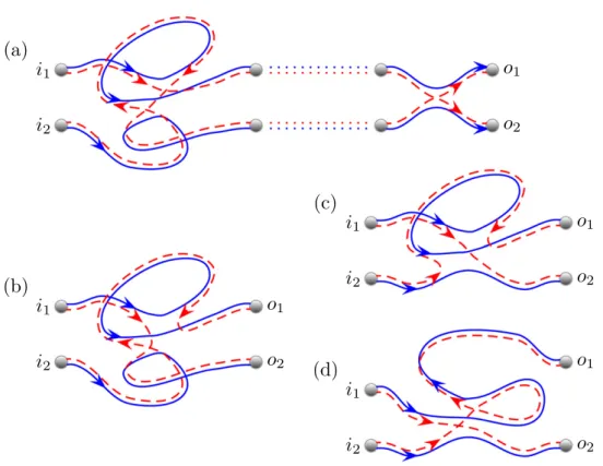
As an example, we discuss the leading order contribution to the second moment m₂. In analogy to transport problems we denote the jth end point by o_j instead of r_j. The simplest trajectory configuration with an encounter is the one that is schematically shown infigure2(a).

The two trajectories belonging toγ are shown by the full lines and go from channel i₁ to end pointo₁and fromi₂too₂, respectively. They have one encounter that is indicated by the circle.

The neighbouring trajectories belonging toγ′(dashed lines) go from i₁to o₂and from i₂too₁, respectively. According to the above rules we obtain the following contribution of this configuration to m₂

μ

−M = − M

T M

1 . (47)

3 4

H 2

2

This contains(−M)from the encounter, M²from the incoming channels,1 M⁴ from the links, and the overall factorT_H² M.

The simpler configuration in figure 2(b) does not usually contribute to m₂ since the trajectories ofγ′(dashed lines) donʼt connect the correct initial and final points. Note, however, that this configuration is possible if the incoming channels coincide. Then one obtains the configuration infigure 3(a). It contributes at the same order as (47) since it has two links, one encounter and one incoming channel less. There is the further possibility that one of the end points is in the encounter as infigures 3(b) and (c), which again contribute at the same order.

All in all the result is

⎛

⎝⎜ ⎞

⎠⎟

μ

−M + + = =

M

M M

M M

T M

T

2 2M 2

. (48)

3

4 2

2 3

H 2

H 2

2 2

This is indeed the leading order term of m₂ in systems with or without TRS.

We have obtained it by considering figures 2(a) and 3(a)–(c) as different trajectory configurations that all contribute to the moment. There is an even simpler and alternative point of view in which one considers all the contributions in (48) to come from figure 2(a). The diagrams in figures 3(a)–(c) are considered to be limiting cases of figure2(a) where either the encounter moves into the incoming lead or one of the end points moves into the encounter.

These limiting cases can be included by changing the contribution of the encounter.

Figure 2. (a) A quadruplet with a single encounter. (b) A quadruplet involving independent links.

Figure 3. Three trajectory configurations that contribute to the leading order of the second momentm2. In (a) the incoming channels coincide, and (b) and (c) have one end point in the encounter. All three are limiting cases offigure 2(a).

For the description we adopt the language from transport and call the initial points of γ i-leaves and the final points o-leaves. For the calculation of the moments m_n we then have to take into account the following cases:

• Encounters of sizelcan move into the incoming lead when connected directly tol i-leaves.

• The o-leaves can be moved into the encounter they are connected to, but each encounter can only take one at a time.

In terms of the semiclassical contributions, in both of these situations we change the rule for the affected encounter to include these cases. In thefirst case we losellinks,(l − 1)channel summations and the(−M)from the encounter, and in the second case we lose one link and the

−M

( ) from the encounter. The contribution of encounter α is hence changed to δ

− + + _α

M( 1 s )withδ being 1 when the encounter can move into the lead (and 0 otherwise) ands_α the number of o-leaves attached.

In our example, if we change the encounter contribution forfigure2(a) in (47) from(−M) toM( 1− +1 + 2) = 2M then we obtain the same result as in (48). One can also easily see that the off-diagonal contributions for the average time delay all vanish, because the last encounter must haveδ = 0(lis at least 2 and there is only 1i-leaf) ands_α = 1 since it is connected to the outgoing channel. The product of contributions is then 0.

We will show below that these rules can be employed systematically to calculate the second moments of the proper time-delays and the variance of the Wigner time delay, and they can as well be incorporated into the graphical framework [62, 63, 77, 87–90] to give moment generating functions. Previous approaches to the time delay involved including an energy dependence so that calculating the semiclassical contribution of any diagram required knowledge of its complete structure. Here instead the semiclassical contributions are much closer to standard transport moments where only the difference in the number of links and encounters matters. The only additional complication is that now some information about the position of the o-leaves is necessary. Determining this is however much less demanding than treating full energy dependence.

3. Second moments

The diagrammatic rules turn semiclassical calculations into a combinatorial problem of counting trajectory configurations (also called structures or diagrams). Before calculating the second moments of various time-delay quantities, we recall that the structures that are relevant for transport moments [59, 60, 91] (and hence also for the time delay) can be related to the structures of periodic orbit pairs that contribute to the two-point correlators in spectral statistics [48–50].

Correlated periodic orbit pairs are also described by a vectorvwhose elementsv_lcount the number of l-encounters of the orbits. The total number of encounters isV = ∑_lvl while the number of links is L = ∑_llvl. The number of periodic orbit structures with a vector v and a labelled first link is N( )v . These numbers can be determined recursively [50].

In the following we deal with systems without TRS. The case of preserved TRS is briefly discussed in section 3.7, being mostly deferred to the appendices.