Dissertation submitted to the Combined Faculties for the Natural Sciences and for Mathematics of the Ruperto-Carola University of Heidelberg, Germany for the degree of Doctor of Natural Sciences

(1)

Dissertation submitted to the

Combined Faculties for the Natural Sciences and for Mathematics of the Ruperto-Carola University of Heidelberg, Germany

for the degree of

Doctor of Natural Sciences

presented by

Dipl. Phys.: Michael Schottner

born in: Heidelberg, Germany

Oral examination: 18

^th

December, 2002

(2)

Algorithms

for the application of

Hartmann-Shack wavefront sensors in ophthalmology

Referees: Prof. Dr. Josef F. Bille

Prof. Dr. Brenner

(3)

Abstract

The topic of this thesis is the development of procedures and algorithms for applications of Hartmann-Shack wavefront sensors in ophthalmology.

Two compact systems were built to do measurements of the entire optical system of the human eye. Automatic pre-correction modules were integrated to compensate a sphere of

−11.25 dpt to 3.25 dpt and an astigmatism of up to 4 dpt.

In the field of image processing, procedures were developed, which allow to recognize strongly aberrated wavefronts. Numerous algorithms are presented, which are suitable to use the extensive raw data to get some significant coefficients. In addition to a modal approach with Zernike Polynomials, alternative possibilities of representation of the wavefront with non-modal and heterogeneous procedures are presented.

Within the framework of this thesis, extensive measuring software was developed. An additional program that simulates image data was developed, with which a great number of parameters can be varied and aberrations in the form of Zernike Polynomials up to 10th arrangement can be used.

In addition to simulations, results of measurements at representative human eyes are presented.

Finally, a conclusion and a view on possible future evolution is given.

Zusammenfassung:

Diese Arbeit befasst sich mit Verfahren und Algorithmen für die Anwendung von Hartmannn- Shack-Wellenfrontsensoren in der Ophthalmologie. Für die Durchführung der Experimente wurden zwei kompakte Systeme aufgebaut, die Messungen der Aberrationen des gesamten menschliches Auges ermöglichen. Zur Erweiterung des Messbereiches wurden automatische Vorkorrektur-Module entwickelt, die Defokus und Astigmatismus kompensieren. Damit sind Untersuchungen an Augen mit einer Sphäre zwischen −11.25 und +3.25 Dioptrien und einem Astigmatismus von bis zu 4 Dioptrien möglich.

Im Bereich der Bildverarbeitung wurden Verfahren entwickelt, die es erlauben, auch sehr stark verzerrte Wellenfronten zuverl¨assig zu erkennen. Zahlreiche Algorithmen werden vorgestellt, die dazu geeignet sind, die umfangreichen Rohdaten auf wenige anschauliche Maßzahlen zu komprimieren. Neben der Entwicklung in Zernike-Polynome werden auch alternative M¨oglichkeiten der Darstellung der Wellenfront mit nicht-modalen und heterogenen Verfahren vorgestellt.

Im Rahmen der Arbeit wurde umfangreiche Messsoftware entwickelt, in die alle behandelten Algorithmen integriert wurden. Zusätzlich wurde ein Programm erstellt, das Messbilder simuliert, bei denen eine Vielzahl von Parametern variiert werden können und Aberrationen in Form von Zernike-Polynomen bis zu 10. Ordnung möglich sind.

Neben Simulationen werden auch Ergebnisse von Messungen an repr¨asentativen menschlich- en Augen vorgestellt.

Abschliessend wird eine Zusammenfassung und ein Ausblick auf denkbare zuk¨unftige Ent- wicklungen gegeben.

(4)

Chapter 1 Introduction

A human gathers most of the information about the environ-

Figure 1.1: Konrad von Soest (1404)

ment with the eyes. Therefore every loss of vision quality hardly influences our daily life. Directly after the invention of the first optical lenses, efforts were undertaken to use them for correction of common refractional errors like nearsighted- ness and farsightedness. Although these early glasses were not suitable to regain full vision with a natural field of view, the benefit for the users was immense.

In the last century, numerous improvements of the glasses were made. New technologies allow to produce thin light- weight glasses with anti-reflex coatings, that mean more com- fort for everyone who wears them. The ability to correct optical errors of the eye is limited by the parameters that are used to manufacture these glasses. This data consists of only a few numbers, that are determined by an optician or op- tometrist. Since the optical properties of individual eyes can vary strongly, not every eye can be fully corrected using these few numbers. New optical products like bifocal and multifocal glasses or soft contact lenses do not exceed these limitations, too.

First efforts to correct individual optical errors were undertaken only in recent years.

New technics of refractive surgery and contact lens design allow to help those people for whom the standard corrections are not sufficient. These correction procedures require detailed information about the aberrations of the eye. The suitable instrument, with which an optician can obtain these information, is the Hartmann-Shack wavefront sensor.

Its optimization is the topic of this thesis.

The second chapter gives a short description of the optical properties of the human eye as far as they are of interest for the understanding of the following chapters. Special attention is given to the anatomical properties, which are important for the optical setup

(9)

2

of the wavefront sensor device. Another part of chapter two is the influence of aberrations like shortsightedness or farsightedness on the visual quality and how they can be corrected.

In chapter 3 the functionality of wavefront sensors is described. After a short overview of the basics of wavefront sensing, the possibilities to compensate strong aberrations within the device is topic of this chapter. The integration of a precompensation of sphere and cylinder in shown.

The optical setup of the devices used for the experiments in this thesis are described in chapter 4. It is started with the basic components and the special requirements for measurements at the human eye. A description of the integration of some extensions follows. Finally, detailed information about the two systems with their special properties is given.

Topic of the fifth chapter are all algorithms, that are used to calculate significant results from the raw data of a wavefront sensor, that consists only of an image with a spot pattern. The main part of the chapter deals with the image procession and the recognition and assignment of the spots. After this, the calculation of wavefront gradients is described.

The chapter concludes with the possibilities to use these gradients to estimate the wavefront and to reduce this wavefront data to some significant values.

These algorithm were integrated in computer programs. All these programs were developed in the framework of this thesis. A full description of the software is given in chapter 6.

The programs are: HSS Analysis 2.x and HSS Analysis 3.x, that are responsible for a complete analysis of wavefront data, HSS Real 1.x, that is optimized for real-time application, and HSS Simulator 1.x, that was used for test of the other three programs.

Chapter 7 shows the results of simulations, that have been done in combination with simulated spot patterns and the analysis software. The first part deals with the effect of general image parameters concerning the image quality to spot finding algorithm. After this, the limits of the algorithm are analyzed. The chapter concludes with an optimization of the algorithm’s speed. The time required for the execution of the time-critical software modules is analyzed and possible accelerations are explained.

In chapter 8 results of measurements at four selected patients are shown. Additional, examples for examinations of time series and spherical aberrations are given.

A summary and a discussion is given in chapter 9. Additionally, some ideas for possible future development are shown.

Two thesis is completed by two appendices. The first appendix gives additional information about the calculation of Zernike Polynomials. Significant software functions are listed in the second appendix.

(10)

Chapter 2 The human eye

Comparing with other optical devices like photo cameras the human eye seems to be a very simple device because it only consists of a few optical components. Nevertheless the human eye is a high performance vision system. The basics of anatomy, physiology and optics of the human eye are described in this chapter as far as it is important for the understanding of the following chapters.

Figure 2.1: Anatomy of the human eye[Atc00]

(11)

2.1 Anatomy of the human eye 4

2.1 Anatomy of the human eye

Four components are of special interest, regarding the optical properties of the eye. These are the cornea, the iris, the crystalline lens and the retina (see fig. 2.1). The dimensions of the components are shown in fig. 2.2.

Figure 2.2: Dimensions of the human eye[Atc00]

2.1.1 Cornea

The cornea is the transparent anterior portion of the fibrous coat of the globe of the eye.

The curvature is somewhat greater than the rest of the globe. The cornea is the first and most important refracting surface of the eye, having a power of 43 D. The anterior surface has a radius of curvature of about 7.8 mm, the posterior surface of about 6.5 mm and the central thickness is about 0.5 mm. It consists of five layers, starting from the outside: (1) the epithelium; (2) Bowman’s membrane; (3) the stroma; (4) Descemet’s membrane and (5) the endothelium. The cornea owes its transparency to the regular arrangement of the collagen fibres, but any factor which affects this lattice structure (e.g. swelling, pressure) results in a loss of transparency.

The anterior surface of the cornea is covered by a tear film of a total thickness of about 10µm. This precorneal film is responsible for a smooth surface of the cornea by compen- sating rough parts of the cornea. Holes in the tear film cause great influence on the optical quality of the eye and lead to complications measuring eyes with wavefront sensors.

(12)

2.1.2 Crystalline lens

Although it has only two optical surfaces, the crystalline lens is the most complex optical component in the eye. It can be seen as an asymmetric deformable biconvex gradient index lens with a refractive index of about n=1.4 in the center decreasing to the periphery. The crystalline lens is the part of the human optical system that is responsible for the accommodation (see fig. 2.3a). Due to increasing size and decreasing flexibility, the maximum amount of accommodation decreases with age (see fig. 2.3b).

a) b)

Figure 2.3: a) The effect of accommodation on the lens shape and lens position, and the principal and nodal points of the eye[Atc00]b) Maximum amount of accommodation as a function of age[Meh96]

2.1.3 Iris

The aperture or opening of the iris is known as pupil. Its size is determined by two antagonistic muscles, which are under autonomic control. The effect of light on the pupil diameter is shown in fig. 2.4b.

An extended pupil has several effects on the vision:

• increasing light level at the retina

• decreasing depth of focus (see fig. 2.4a)

• increasing diffraction-limited resolution

• more or less dislocated visual axis with all resulting effects

(13)

a) b)

Figure 2.4: a) Pupil diameter as a function of light level[Atc00] b) Depth of focus as a function of pupil diameter[Meh96]

2.1.4 Retina

The light-sensitive tissue of the eye is the retina. It consists of a number of cellular and pigmented layers and a nerve fibre layer (see fig. 2.5a). The light sensitive cells are placed at the back of the retina. Light must pass through the other layers to reach these cells.

There are two types of these cells, known as rods and cones. The cones predominate in the fovea, that is responsible for the highest visual acuity in the eye, and are responsible for color vision and vision at high light level (photopic vision). The rods are responsible for the vision at low light levels and are not sensible for color vision (scotopic vision). The distribution of rods and cones in the retina is shown in fig. 2.5b.

Stiles-Crawford Effect

Stiles and Crawford discovered, that the luminous efficiency of a beam of light entering the eye and incident on the fovea depends upon the entry point in the pupil. This effect is important to retinal image quality and is a consequence of the wave-guide properties of the photoreceptors. It is predominantly a cone phenomenon, and hence predominantly a photopic phenomenon. As a result of this effect, optical aberrations in the periphery affect the vision less than aberrations near the visual axis.

(14)

2.2 Transmittance of the optical media 7

a) b)

Figure 2.5: a) The layers at the back of the human eye building the retina[Atc00]b) The density of cones and rods across the retina in the temporal direction[Atc00]

2.2 Transmittance of the optical media

For all optical diagnostic methods in the human eye, the transmittance of the whole eye is very important. In figure 2.6 you can see that the eye is almost transparent for electro- magnetic waves with a wavelength between 450 and 1200 nm. This fact makes it possible to use invisible light from the infrared spectrum for diagnostic and surgical applications in the eye.

Figure 2.6: Transmittance of the human eye[Atc00]

(15)

2.3 Reflectance of the retina 8

2.3 Reflectance of the retina

Optical instruments like the wavefront sensor, discussed in the following chapters use the light reflected by the retina. In figure 2.7 the spectral reflectance of the fundus is shown.

One can see, that light with a wavelength above 600 nm can be used for this kind of measurements.

Figure 2.7: Spectral reflectance of the fundus[Atc00]

2.4 Main refractional errors

The refractive state of the eye which focuses distant objects on the retina while the lens is relaxed, is called emmetropia. Most of the human eyes don’t match this condition. They have one or more refractional errors. The most common refractional errors are described in the following section.

Figure 2.8: Emmetropia: In a relaxed eye distant objects are focused on the retina.

(16)

2.4 Main refractional errors 9

2.4.1 Myopia

Myopia is the refractive condition of the eye, in which the images of distant objects are focused in front of the retina, when accommodation is released (fig. 2.9a). It is also known as shortsightedness. Emmetropia can be achieved by decreasing the optical power of the optical system (fig. 2.9b).

a) b)

Figure 2.9: a) Myopia: In a relaxed eye distant objects are focused in front of the retina.

b) Myopia corrected with a negative lens

2.4.2 Hyperopia

Hyperopia is the refractive condition of the eye, in which the images of distant objects are focused behind the retina, when accommodation is released (fig. 2.10a). It is also known as farsightedness. Emmetropia can be achieved by increasing the optical power of the optical system (fig. 2.10b).

a) b)

Figure 2.10: a) Hyperopia: In a relaxed eye distant objects are focused behind the retina.

b) Hyperopia corrected with a positive lens.

2.4.3 Astigmatism

Astigmatism is the condition of refraction, in which the image of a point object is not a single point but two focal lines at different distances from the optical system. In most astigmatic eyes the refractive power of the vertical meridian (with the rule) or the horizontal meridian (against the rule) is the greatest.

(17)

2.4 Main refractional errors 10

2.4.4 Spherical Aberration

The spherical aberration is a defect of the optical system due to a variation in the focusing between peripheral and paraxial rays. The larger the pupil size, the greater the difference in focusing between two rays. When the peripheral rays are refracted more than the paraxial rays, the aberration is said to be positive or undercorrected. When the peripheral rays are refracted less than the paraxial rays, the aberration is said to be negative or overcorrected.

The relaxed eye has a small amount of positive spherical aberration (up to 1 dpt for pupil of 8 mm)[Mil98].

2.4.5 Chromatic Aberration

Like other optical systems, the eye suffers from chromatic aberrations as well as from monochromatic aberrations. This is caused by the different focus lengths of light with different wavelength. The effect of wavelength on refraction is shown is fig. 2.11.

Figure 2.11: Results of experimental studies of chromatic difference of refraction as function of wavelength.[Atc00]

(18)

2.5 Visual Acuity 11

2.5 Visual Acuity

The Visual acuity is capacity for seeing distinctly the details of an object. It can be quantified as the reciprocal of the minimum angle of resolution (in minutes of arc), that can be measured using a vision chart with Landolt rings, Snellen test types or equivalent objects (see fig. 2.12).

a)

b) c)

Figure 2.12: a)Snellen test types b)Landolt broken ring c)Snellen vision chart All aberrations have an influence on the visual acuity. A relationship between uncorrected hyperopia/myopia and visual acuity is shown in fig. 2.13b and 2.13c. The influence of astigmatism on the visual acuity is shown in fig. 2.13a. You can easily see, that the effect of astigmatism on the visual acuity is approximately 50 percent of those caused by hyperopia or myopia. Another parameter that influences the visual acuity is the eccentricity (see fig.

2.13d). An eccentricity of 5 degrees corresponds to myopia and hyperopia with 1 dpt and or an astigmatism of 1.75 dpt. Finally there is an influence of the age (see fig. 2.14).

(19)

2.5 Visual Acuity 12

a) b)

c) d)

Figure 2.13: Relationship between visual acuity and a)uncorrected astigmatism b) uncorrected hyperopia c)uncorrected myopia d)eccentricity [Mil98]

Figure 2.14: Relative visual acuity in dependence of the age[Meh96]

(20)

2.6 Corrections of the optical aberrations 13

2.6 Corrections of the optical aberrations

2.6.1 Eye glasses

The oldest and most common possibility for a correction of the refractional errors of the human eye are eye glasses. The first glasses are designed only for a correction of nearsight- edness and farsightedness and had only one refracting surface with an spherical shape.

Later spectacles have two refracting surfaces, one spherical and one cylindrical surface.

Up–to–date spectacles have a toric surface instead of a spherical. The newest development in the spectacles research are bifocal and multifocal glasses.

There is one important limitation to all spectacles: they are only designed for the correction of sphere and cylinder. Additionally especially when glasses with high power are used, higher aberrations are created for off–axis.

The parameters needed for the shaping of a spectacles glass are the sphere in diopters, the cylinder measured in diopters with the angle to the vertical. Additionally the distance from the glasses to the eye is needed.

2.6.2 Contact lenses

Another possibility of correction of refractional errors in the eye is the contact lens. They are available as hard, hard–flexible or soft lenses for daily, monthly or permanent use.

Most contact lenses are only suitable to correct myopia and hyperopia. Hard lenses are also suitable to correct smaller aberrations caused by the anterior surface like astigmatism of up to 1 dpt. Modern self–stabilizing soft lenses are also able to correct higher amounts of astigmatism. Future contact lenses will be able to correct higher order aberrations. They have to be manufactured individually for every patient and require data of all aberrations of the eye. A suitable device for the required measurements is the wavefront sensor.

2.6.3 Refractive surgery

Permanent correction of aberrations can be achieved also by refractive surgery. Current surgical technics are PRK (Photo Refractive Keratectomy) and LASIK (Laser in situ Keratomilieusis). Latest clinical studies showed, that aberration–free refractive surgery is possible[Bil02]. Corrections of higher order aberrations also require wavefront data.

(21)

Chapter 3 Principles of wavefront sensors

3.1 Hartmann test

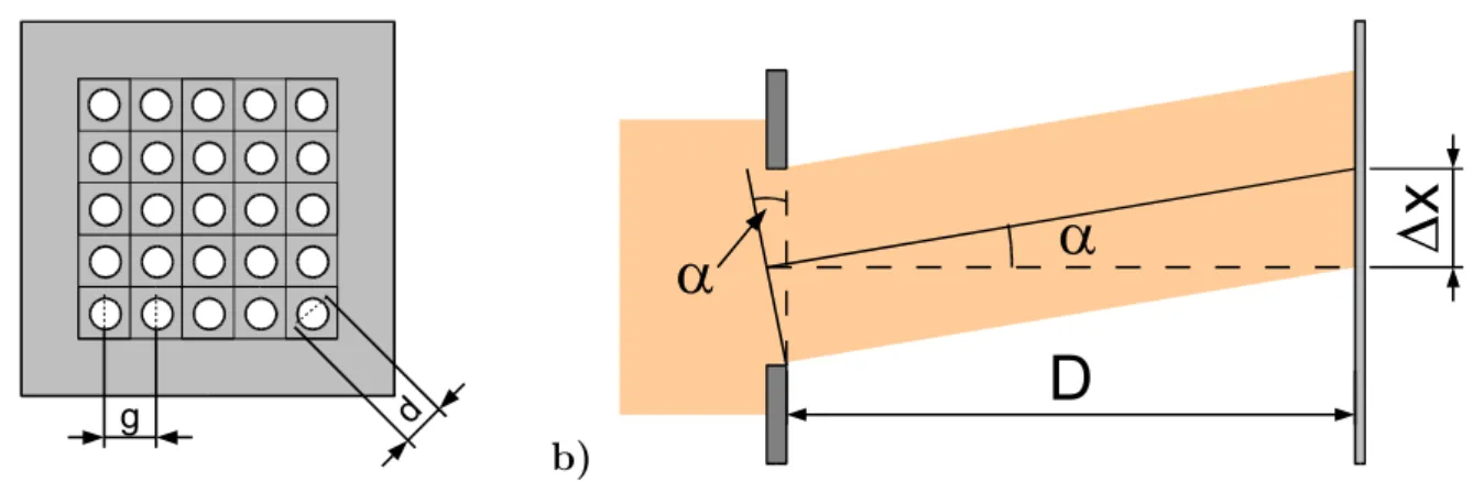
A simple method used in wavefront diagnostics is the Hartmann test. It consists of two parts. The first part is a plate with a hole pattern, placed in the plane where the wavefront should be sensed. Behind the plate the wavefront is divided in a number of small parts.

Every part of the wavefront could be seen as a single approximately plain wavefront with a homogeneous direction of propagation.

hole plate screen

incoming wavefront

Figure 3.1: 2-dimensional Hartmann test

In a distance D behind the hole plate a plain screen is placed. For automatic wavefront analysis, a camera chip can be used as screen.

(22)

3.1 Hartmann test 15

a)

g d

b)

a D

D x

a

Figure 3.2: a) The Hartmann screen front viewb) Geometric properties of one subaperture

The shift ∆xof the center of the light spot on the screen is proportional to the local tilt of the wavefront W at the hole plate.

α_x ≈tan(α_x) = dW(x, y)

dx = ∆x

D ; α_y ≈tan(α_y) = dW(x, y)

dy = ∆y

D (3.1)

Two neighboring spots on the screen overlap, if the lateral shift of one point equals:

∆xmax=g−d (3.2)

This corresponds to an maximum angle α of:

αmax≈= tan

g−d D

(3.3) The principle used in this kind of sensor has several limitations:

• A big fraction of the light is blocked by the hole plate.

• The intensity within the spots is at the most just as high as within the original wavefront.

• Small shift of the spots may cause overlapping.

• No information can be obtained about the wavefront at the blocked areas.

(23)

3.2 Hartmann-Shack wavefront sensor 16

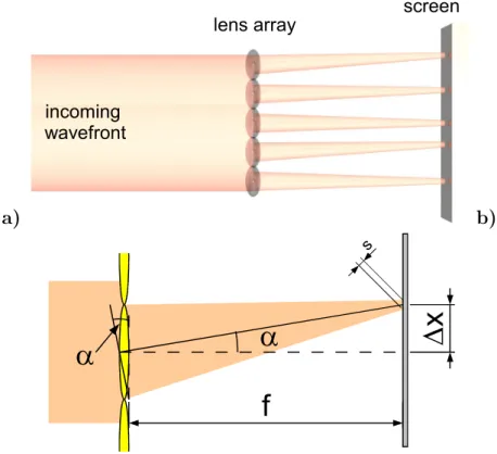
3.2 Hartmann-Shack wavefront sensor

The Hartmann-Shack wavefront sensor uses a principle similar to the Hartmann test[Sha71].

The only difference is a 2-dimensional array of lenses that replaces the hole plate. Instead of the variable distance D, the distance between lens array and screen has to be equal to the focal length of the lenses in the array.

a)

lens array screen

incoming wavefront

b)

a f

D x

a

s

Figure 3.3: a)2-dimensional Hartmann-Shack wavefront sensor (HSS)b) Geometric properties of one subaperture

For the lateral shift of the focus spots exists a similar equation:

α_x ≈tan(α_x)dW(x, y)

dx = ∆x

f ; α_y ≈tan(α_y)dW(x, y)

dy = ∆y

f (3.4)

Since the size of the focus spots s can be much smaller than the size d of the holes of the Hartmann hole plate, overlapping is less probable.

(24)

3.3 Extensions of the HSS 17

3.3 Extensions of the HSS

If it is not possible to place the lens array in the plane where the wavefront should be detected, a telescope is necessary (see fig. 3.4). The detection plane and the sensor plane are conjugated to each other.

P

f

1

f

1

f

2

f

2

L

Figure 3.4: HSS with a telescope. For equal values of the focal lengths f1 and f2, the wavefront at the position of the plane Pis equal to the wavefront at the lens array L.

If lenses with different focal lengths are used, the telescope is suitable to magnify the wavefront in lateral direction. A point A_P(x_P, y_P) in the plane P is imaged to A_L(x_L, y_l) in the plane of the lens array L with:

x_L=−x_P · f₂

f₁ ; y_L =−y· f₂

f₁ (3.5)

The gradient (dW(x_P, y_P)/dx_P, dW(x_P, y_P)/dy_P) at P corresponds to an gradient (dW(x_L, y_L)/dx_L, dW(x_L, y_L)/dy_L) at L with:

dW(xL, yl)

dx_L =−f1

f₂

dW(xP, yP)

dx_P ; dW(xL, yl)

dy_L =−f1

f₂

dW(xP, yP)

dy_P (3.6)

The optical path difference is not affected by the telescope since the product of lateral magnification and magnification of the gradient is independent of the ratio betweenf₁ and f₂.

If more than one telescope is put in the optical path, the resulting magnification is the product of all single magnifications. The planes between the telescopes are again conjugated to the sensor plane and the detection plane.

(25)

3.3.1 General compensation of aberrations

The dynamic range of HSS is limited by its focal length and sub-lens diameters. The sensitivity of the wavefront sensor for small aberrations limits the maximum measurable aberrations. A common case is a wavefront with high values of sphere or astigmatism and small additional higher order aberrations. A solution for this kind of wavefronts is a defined precompensation of sphere and astigmatism.

A general approach for compensation of any aberration is to put a correcting element between two telescopes in a plane P₁ that is conjugated to the sensor plane and to the detection plane (see fig. 3.5). The correcting element at P₁ can be any kind of thin lens.

The positions of the wavefront at the sensor plane L corresponds to the following position at the detecting plane P:

x_L=x_P · f₂ f₁

f₄

f₃ ; y_L=y· f₂ f₁

f₄

f₃ (3.7)

and to the position at the compensation plane P₁: x_L=−x_P · f₄

f3

; y_L =−y· f₄ f3

(3.8)

P

f1 f1 f2 f2

L

f3 f3 f4 f4

P¹

Figure 3.5: General compensation of aberrations. The phase plate P₁ directly affects the wavefront at the sensor L.

With this optical setup, it is possible to compensate any amount of sphere by putting a positive or negative lens into the beam at position P₁. If two 1:1-telescopes are used, a wavefront with a positive/negative sphere can be compensated by a negative/positive lens with the same amount at the position P1. If the sphere is the only aberration, the result will be plain wave at the sensor plane L.

Similar results can be achieved with a compensation of astigmatism. A cylinder lens has not only an astigmatic component but also a sphere component. Therefor compensation of pure astigmatism requires at least two elements: a cylinder lens and a spherical lens or two cylinder lenses.

(26)

3.3.2 Sphere compensation

A more flexible setup for a compensation of sphere is to modify the distance between the two lenses of a telescope (see fig. 3.6). The effective power 1/g of a telescope extended by a d can be calculated with the lens equation:

1

f₁ = 1

f₁+d + 1

f₁−g (3.9)

The solution for the effective power is:

1 g = d

f₁² (3.10)

If the focal lengthf₁ is 50 mm, for example, the effective power D is:

D= 1

g = d

(50 mm)² = d

2.5 mmdpt (3.11)

With this result, you can say that every 2.5 mm translation corresponds to a compensation of 1 diopter.

P

f

¹

f

¹

f

²

f

²

L

d

Figure 3.6: A telescope used for correction of sphere.

3.3.3 Cylinder compensation

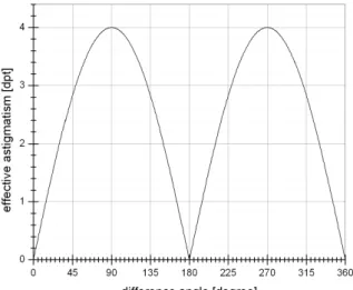
Although it is possible to put a cylinder lens with the desired power and axis between two telescopes as shown in fig. 3.5, a more flexible solution is preferred. Instead of a single cylinder lens, a pair of two cylinder lenses with the same amount of power (P_1,2) but opposite sign can be used.

(27)

Figure 3.7: Two rotating cylinder lenses suitable to compensate astigmatism with any power and any axis.

If the angle between the axes of the two cylinders lenses is zero, the resulting effective cylinder has 0 dpt. A rotation of the two axes against each other cause an effective cylinder of up to twice the power of one cylinder lens at the 90^◦-position. If the rotation angle of the first, positive lens is α₁ and the rotation angle of the other cylinder lens is α₂, the resulting astigmatism has the power:

P_effective = 2·P_1,2· |sin(α₁−α₂)| (3.12)

The angle of the resulting astigmatism is:

α_effective = α₁+α₂

4 −45^◦ (3.13)

Higher order aberrations caused by this setup are very small for distances between the two cylinder lenses that are small in comparison with their focal lengths.

Figure 3.8: Effective astigmatism as result of two rotated cylinder lenses with focal lengths of 500 mm and -500 mm.

(28)

Chapter 4 Optical setup of the devices

For the tests of the algorithms and applications at human eyes two complete systems have been build. The first system is a small device with sphere compensation that is suitable for clinical application. The second system has been built for experimental purposes. It has a build-in compensation of sphere and cylinder, and is based mainly on LINOS Microbench.

Three additional copies of the first system have been built in cooperation with Philips to do extended clinical studies. Experiences with these systems have been used to improve the reliability of the algorithms especially with problematic eyes.

In the first part of this chapter, the basic components of the devices are described. The extensions, that are part of both systems, are topic of the following section. The chapter concludes with descriptions of the two systems with their individual extensions.

4.1 Basic components of the wavefront sensors

The basic setup for all systems is shown in fig. 4.1. The necessary components are the wavefront sensor, consisting of a lens array and a camera chip, the light source, a beam splitter and a telescope consisting of two lenses.

For applications at the human eye the wavefront sensor has to fulfill several conditions:

• The lateral extension of the wavefront sensor should match to the size of the wavefront limited by the pupil of the eye (diameter about 2-7 mm).

• The number of rows and columns of sublenses used for the measurements should allow the determination of higher order aberrations. In combination with the previous condition the size of the sublens is limited to values smaller than 400µm to have at least 5 rows and columns usable for the reconstruction of the wavefront.

• A light source should have a wavelength that will be transmitted by the optical media of the eye and that will be reflected by the retina. Furthermore, the spectral

(29)

4.1 Basic components of the wavefront sensors 22

E

LD L1 LA

Figure 4.1: Basic components for measurements with a HSS at the human eye. The beam of the light source LD is reflected by a beam splitter into the optical axis of the system.

The parallel beam is focused on the retina by the eye E. The two lenses L1 and L2 are necessary for a lens arrayLAthat is conjugated to the pupil plane of the eye. The camera C1 detects the HSS spot pattern.

sensitivity of the retina for this wavelength should be low to avoid blending of the patient.

• The light intensity should be less than the maximum intensity allowed for long-time exposure of the human eye to an collimated beam.

4.1.1 Lens array

The properties of the lens array determine the sensitivity, the dynamic range and the lateral resolution of the HSS. The first parameter is the distance between the sub lenses that should be equal to their diameter. A sub lens diameter of 300-400µm allows to use about 15-20 rows and columns of the lens array with a 6 mm pupil. The smallest standard lens arrays available have a total diameter of 0.5⁰⁰ or 1⁰⁰, so they cover more than the 7 mm of the maximum wavefront’s lateral extension. The focal length is responsible for the dynamic range of the sensor. Values between 30-50 mm are a good compromise between higher sensitivity and larger dynamic range. The parameters of the lens arrays used in the systems are shown in table 4.1.

No. sub lens diameter focal length

1 400µm 53 mm

2 312.5µm 34 mm

3 300µm 30 mm

Table 4.1: Main parameters of the lens arrays used for the experiments

(30)

4.2 Extensions of the wavefront sensors 23

4.1.2 Light source

For best results a collimated monochromatic light source is required. The best solution is a diode laser, that is small, adjustable and that emits light with the described qualities. The next question is the choice of a wavelength. Light with a wavelength in the near infrared is transmitted by the optical medias of the eye and reflected by the retina and doesn’t blend the patient. A wavelength of 780 nm is a common wavelength for diode lasers and is almost invisible because of the low spectral sensitivity of the eye (see chapter 2).

4.1.3 Camera

The camera is responsible for the image acquisition. Since most standard ccd cameras are still sensitive for light with this wavelength, a special infrared camera is not required.

Cameras with standard ccir video output have a sufficient resolution of 768×576 pixels.

Devices with higher resolutions and smaller pixel dimensions are less sensitive and require special expensive image acquisition hardware. A critical parameter is the frame rate of standard cameras: A maximum number of 25 frames (50 half frames) can be taken in one second. Fast eye movements like micro saccades require much more frames per second, but for most situations the standard 25 frames are sufficient. The size of a camera with 2/3⁰⁰-chip (8.8 mm×6.6 mm) perfectly fits to size of the pupil-limited wavefront.

4.2 Extensions of the wavefront sensors

4.2.1 Laser monitoring

Although the laser diode has an internal system for power monitoring, an additional external system is required for security reasons. The light intensity at the eye should not exceed a power of 50µW. If the laser output increases or decreases, the power is automatically turned off and requires a manual reset for restart.

4.2.2 Polarization elements

Some components used in the systems concern the polarization, that is required for the suppression of reflection. Although all optical surfaces have an anti-reflex coating, reflections are still present. Since only a small part of the incoming light is reflected by the eye, some reflection of surfaces in the system have a similar intensity. All reflections can be reduced using polarized light. The laser diode emits light that is almost linear polarized.

The polarizing beam splitter B2 only reflects linear polarized light. All the light reflected be the surfaces between this beam splitter and the quarter wave plate in front of the eye have the same polarization. The polarizing beam splitters B2 and B3 reflect this light and

(31)

4.3 Optical setup of System 1 24

insure, that it doesn’t reaches the camera C1. Light that passes the quarter wave plate is circular polarized and linear polarized orthogonal to the incoming light after the second pass. This light is transmitted by B2 and B3 and can be detected by the camera C1. The quarter wave plate is tilted to avoid reflections from its left surface.

Figure 4.2: Complete schematic setup of the whole systems including mechanical components and data processing. The observation system is not present in the first system, the cylinder compensation is not present in the second system.

4.3 Optical setup of System 1

In the first system, the following extensions are implemented: the laser monitoring, the polarizing elements, a pinhole for spacial filtering, a sphere compensation and a pupil observation system (see fig. 4.4).

4.3.1 Pinhole

The pinhole PH removes most of the reflections from the cornea. An additional effect of the pinhole is that wavefronts with more than 0.75 dpt are blocked. This is not a problem because most of the sphere can be removed by the sphere compensation system.

4.3.2 Pupil observation system

Reproducible measurements at the human eye require a precise lateral and axial fixation of the pupil. Lateral translations of the eye cause lateral translations of the HSS pattern

(32)

Figure 4.3: Picture taken with the observation camera

on the camera chip with the same amount. Since the camera chip has a size of 6.6×8.8 mm it is necessary that a 6 mm-pupil has to be aligned with a accuracy of better than 0.6 mm to avoid loss of information. The focus plane of the lens L1 is conjugated to the plane of the wavefront sensor. Since L1 and L2 have an identical focal length, these wavefronts are identical. Axial translations away from these positions make it extremely difficult to determine the shape of the wavefront at the eye.

For these two issues an additional observation camera (see green beam in fig. 4.4) is implemented in the system. A picture taken with this camera is shown in fig. 4.3. The device is aligned, if the pupil is centered and the iris of the eye is sharp recognizable. Due to a small depth of focus of the observation camera system, axial translation smaller than 1 mm can be observed. The whole system can be moved in all directions by an operator using the joystick (see fig. 4.5a).

4.3.3 Sphere compensation

The sphere compensation is implemented as it is described in the previous chapter. The right part of the system showed in fig. 4.4 is movable by an motorized translation stage. It seems, that is could be easier to move the left part. Since a defined distance between the eye and the lens L1 is required, the patient would have to be moved too. The compensation D can be calculated using the focal length of 50 mm:

D= d

(50 mm)² = d

2.5 mmdpt (4.1)

The range is limited by the available space. A maximum translation range of 36.25 mm corresponds to a difference of 14.5 dpt that is used to compensate spheres with a power of

−11.25 dpt to +3.15 dpt.

(33)

4.3.4 Optical setup

The optical setup of system 1 is shown in fig. 4.4. The whole device is put in a compact box and mounted movable on a chin rest (see fig. 4.5).

E

B1 LD C2 PD

L4

Figure 4.4: Optical setup of HSS system with sphere compensation. The light emitted by the laser diode LD is split by the polarizing beam splitter cube B1, that improves the polarization of the beam and that enables the photodiode PD to monitor the laser output. The second beam splitter cube B2 reflects the laser beam into the optical axis of the system. The two 50 mm-achromats L1 and L2 build the telescope, that is responsible for the conjugation of the pupil plane with the sensor plane. The quarter wave plate λ/4 converts the polarized light to circular polarized light. The eye E focusses the light on the retina where it is reflected. The reflected light is linear polarized after the second pass of the quarter wave plate λ/4. The pinhole PH filters reflections caused by the cornea.

The polarizing beam splitter cubes B2 and B3 filter all reflections that haven’t passed the quarter wave plate λ/4. The lens array LA and the camera C1 form the wavefront sensor. The cmos camera C2, the 20 mm lens and the mirror S1 are components of the pupil observation system. The right part of the system can be translated against the left part with a motorized translation stage.

(34)

a) b)

Figure 4.5: a) Photography of system 1 b) system 1 mounted on a chin rest

4.4 Optical setup of System 2

In the second system, the following extensions are implemented: the laser monitoring, the polarizing elements, a compact sphere compensation (fig. 4.6) and a cylinder compensation (see fig. 4.8).

4.4.1 Sphere compensation

a)

P2

b)

P2

Figure 4.6: Sphere compensation modulea)in home positionb)in compensation position The sphere compensation in system 2 is little different to the previous one. Instead of moving almost the whole system, only a prism is moved (see fig. 4.6). Every millimeter of translation d of the prism P2 causes a change of the telescope length of 2 millimeters.

(35)

With the 50 mm-lens L1 the resulting compensationD is:

D= 2, d

(50 mm)² = d

1.25 mmdpt (4.2)

4.4.2 Cylinder compensation

The cylinder compensation used in system 2 is realized as mentioned in the previous chapter. Since the two telescopes have no magnification, the compensation at the eye, at the lens array and at the cylinder lenses are equal. The cylinder lenses have focal lengths f_c1, f_c2 of +500 mm and -500 mm. The maximum astigmatism compensation D_a is:

D_a = 1 1 f_c1 − 1

f_c2 = 1

500 mm + 1

500 mm = 4 dpt. (4.3)

The two lenses are individually mounted in motorized rotation stages. It is possible to rotate every cylinder lens with 720^◦/s with a precision of better than 0.1^◦. The required rotation for both cylinder lenses to change the compensation from 0 to 0.5 dpt is:

α₁ =−α₂ = arcsin

0.5 dpt 4 dpt

45^◦ = 5.61^◦ (4.4)

A rotation of 5.61^◦ of both cylinders takes less than 10 ms. The mechanical realization of the cylinder compensation is shown in fig. 4.7.

Figure 4.7: Cylinder compensation module

(36)

4.4.3 Optical setup

The optical setup of system 2 is shown in fig. 4.8. A picture of the mechanical setup is shown in fig. 4.9

E l/4 PH

B1 LD P2

PD

Figure 4.8: Optical setup of HSS system 2 with compensation of sphere and astigmatism.

The light emitted by the laser diode LDis split by the polarizing beam splitter cube B1, that improves the polarization of the beam and that enables the photodiode PD to monitor the laser output. The second beam splitter cubeB2reflects the laser beam into the optical axis of the system. The four 50 mm achromats L1,L2,L3 and L4 build two telescopes, that are responsible for the conjugation of the pupil plane with the sensor plane. The two cylinder lenses Z1 and Z2 with focal lengths of 500 mm and -500 mm are individual motorized 360^◦ rotatable and build the astigmatism compensation system. The prism P1 and movable prismP2build the sphere compensation system. The quarter wave plateλ/4 converts the polarized light to circular polarized light. The eye E focusses the light on the retina where it is reflected. The reflected light is linear polarized after the second pass of the quarter wave plate λ/4. The pinhole PH filters reflections caused by the cornea.

The polarizing beam splitter cubes B2 and B3 filter all reflections that haven’t passed the quarter wave plate λ/4. The lens array LA and the camera C1 form the wavefront sensor. The cmos camera C2, the 20 mm lens and the mirror S1 are components of the pupil observation system.

(37)

Figure 4.9: Mechanical setup of system 2

(38)

Chapter 5 Algorithms for the use with wavefront sensors

The topic of this chapter is the whole process starting from the data delivered by the framegrabber and ending with the presentation of the wavefront and refraction data. This process can be divided in several parts. The first part is the image processing with the image preprocessing and the spot finding algorithm. After a successful spot finding process the acquired data of the spot positions can be used for modal or zonal estimation of the wavefront. With this wavefront data numerous interesting parameters like the sphere, astigmatism or spherical aberration can be calculated easily.

5.1 Image preprocessing

The first task of the image processing is the analysis of the image quality. For best results in the following steps, it is necessary that the available 8 bits of the framegrabber are used optimally. The most problems can be recognized easily using the raw data.

A great number of pixels having the maximum available gray level (255) is a clear sign that the framegrabber achieved a level of saturation. This causes a loss of information for the following spot finding process because the pixels in the center of the spots with saturation won’t help increasing the precision on the spot position. An example a spot pattern with obvious saturation is shown in fig. 5.1. There are three solutions to solve this problem for the next images that will be taken. The first possibility is to increase the white level of the framegrabber. This can be easily done using the software interface of the framegrabber. The next solution is to decrease the sensitivity of the ccd camera. This can also be done automatically by the software if the camera has a suitable interface to the computer. The last possibility is to decrease the laser power. Since the applicable laser light level used for diagnostics at the human eye is already extremely low, adjustments of the laser power in not useful in this case.

(39)

5.1 Image preprocessing 32

a) b)

Figure 5.1: A spot pattern with perfect adjustment of framegrabber, camera sensitivity and laser power. The dynamic range is used optimally. a)part of spot pattern b)2-d-plot of gray values

a) b)

Figure 5.2: Part of a spot pattern with the framegrabber reaching a level of saturation a)Part of spot patternb)2-d-plot of gray values

The opposite problem is low intensity which means that the maximum gray level in the image is by far less than the maximum gray level available, which also causes less precision in the whole data. A solution can be found similar to the problem with the saturation (see fig. 5.2).

The third problem is a high minimum gray level, that is a obvious sign for a high underground level (see fig. 5.3 ). It can be caused by a low black level of the framegrabber or a high camera sensitivity. An adjustment of the framegrabber by the software is the preferred solution also for this problem but camera adjustment is also possible. If a high underground gray level is present, the spot finding algorithm will take much more time and it is possible that some spots can’t be recognized correctly.

If most of the pixels in the image have a gray level of zero (black), parts of spots or whole spot could be missing (see fig. 5.4). The solution is a decreasing of the framegrabber black level or the increasing of the camera sensitivity.

These four problems mainly concerning the framegrabber sensitivity are summarized in table 5.1 with its identifying parameters.

Completely different to the previous four cases is a spot pattern like that in fig. 5.5.

It shows saturation of the camera. It can easily recognized by numerous pixels with very

(40)

5.1 Image preprocessing 33

a) b)

Figure 5.3: Part of a spot pattern with with low intensity. Only the lower range of the dynamic range of the framegrabber is used. Precision is lost a)Part of spot pattern b)2- d-plot of gray values

a) b)

Figure 5.4: Part of a spot pattern with high black level of the framegrabber. The lower parts of the spots are missing. It is also possible, that darker spots are completely missing.

a)Part of spot patternb)2-d-plot of gray values

Case max. gray level % of pixels with min. gray level % of pixels with in image max. gray value in image zero gray level

perfect pattern ∼255 <0.1 0 0−50

saturation 255 >0.1 - -

low light <200 0 - -

high underground - - >0 0

black image - - 0 >50

Table 5.1: Summary of the parameters identifying the four cases of required adjustments of the black and white levels in the framegrabber responsible for the quality of the spot patterns. All values are the result of numerous tests with different conditions and could vary for different setups

(41)

5.2 Spotfinding algorithms 34

a) b)

Figure 5.5: A spot pattern with saturation of the cameraa)part of spot patternb)2-d-plot of gray values

a) b) c)

Figure 5.6: Example for removing stationary artifacts by subtracting images. a)detail of original imageb)detail of original image without HSS pattern c)detail of image after difference

similar gray values in the center of each spot. This problem can’t be solved by adjusting the parameters of the framegrabber. A decreasing of the incoming light level is necessary.

This can be corrected by adjusting the laser power or by using a gray filter. With the optical setup used for all the measurements, spot patterns from human eyes will never produce light levels at the camera that are nearly that high.

In some optical setups additional reflections caused by optical components are unavoid- able. If they are stationary and their intensity does not exceed the intensity of the real HSS spot pattern, it is possible to remove them by software. For this task an image without HSS pattern is required to build the difference (see fig. 5.6).

5.2 Spotfinding algorithms

The most important part of the image processing with HSS spot patterns is the spot finding algorithm. It consists of the recognition of the focus points, the determination of the position of the centers and the assignment of these points to the corresponding subapertures.

(42)

a) b)

Figure 5.7: A spot pattern with perfect adjustment of framegrabber, camera and laser a)part of spot pattern b)2-d-plot of gray values

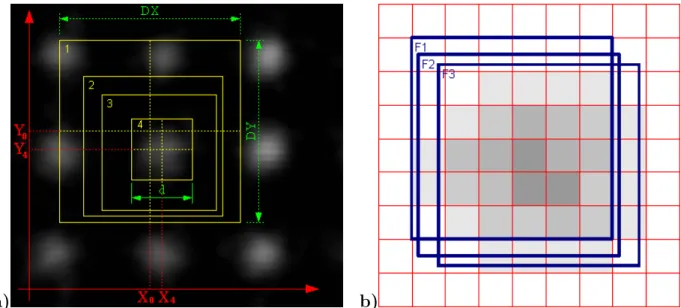
5.2.1 Spot centering

The spot centering algorithm is part of all the following strategies. After an area of the image is chosen where one spot is expected, this algorithm starts. The required parameters are the position of the expected spot (X, Y),the size of the frame (DX, DY) that should be used for this centering procedure and the maximum diameter of the spots (D). The centering procedure is based of a number of iterative calculations of the center of mass of the gray values (G_i) where the result of the previous step is used as starting point for the next step.

¯ x= 1

n

X

i=1

G_i·x_i; y¯= 1 n

n

X

i=1

G_i·y_i (5.1)

The iteration consists of two phases. The first phase starts with a frame size of (DX, DY) and continues with smaller frames down to the expected size of the spots (see fig. 5.7a) ). After 3-10 iterations this phase can achieve a accuracy of about 1 pixel (∼ 10µm).

For better results the second phase with constant frame size continues with another 10-50 iterations. Simulations with different images showed that the number of required iterations decreases with better image quality. Images with very much noise and a high underground level showed that even after 50 iterations the spot position could change a little bit with further iteration s.

For better results the centering process can be extended by using fragments of pixel[Mue01].

An example for this process with sub pixel accuracy is shown in fig. 5.7 b).

(43)

a) b)

Figure 5.8: A spot pattern with perfect adjustment of framegrabber, camera and laser a)part of spot pattern b)2-d-plot of gray values

5.2.2 Static spotfinding

The first approach for the spotfinding strategy is to use a fixed grid to find the spots. This procedure requires the assumption that no spot can move as much as half the distance between two subapertures. Once started with one frame only a few iterations are required to find the spot because you can be sure that only pixels of one spot are within the frame and this frame is the correct one. This procedure fails if one spot has moved more than half the distance because a correct assignment is not still possible (fig. 5.8a). This means a strong limitation to the processable wavefronts. For an optical setup using an lens array with a distance between the subapertures of 400µm and a focal length of 53 mm the maximum spot translation is 200µm and the maximum local wavefront tilt is about 0.2 degree. Similar tilts appear in the external fields of an wavefront with a diameter of 6 mm and a sphere of about 1 dpt. Astigmatism and higher order aberrations as they are present in many human eyes are often responsible for additional tilts with the result that the dynamic range of the wavefront sensor is limited to wavefronts less than this 1 dpt.

Measurements at human eyes using the static spotfinding algorithm require good alignment of the eye in addition with good precompensation of the main refractional errors.

5.2.3 Adaptive spotfinding

For spot patterns that don’t look almost like a spot pattern generated by a plane wave a more intelligent spotfinding algorithm is required. It should allow the recognition and assignment of spots like those in fig. 5.9. Although these spot patterns doesn’t match to any fixed grid, nobody should have a problem to assign all visible spots correctly. The approach of the adaptive spotfinding algorithm is to imitate the way a human would assign the spots. The easiest way is to look for something that looks like the expected pattern.

This can be found most likely in the center of the whole pattern where the distance between

(44)

a) b)

Figure 5.9: Spot patterns from distorted wavefronts that can’t be processed by the static spotfinding algorithma) High spherical aberrationb) Human eye with strong aberrations

a) b) c)

Figure 5.10: Different paths of the searching process. a)starting with vertical search, then horizontal b) starting with horizontal search, then vertical. The algorithm uses both and compares the results. If there are any differences, the search will be repeated with modified parameters. c) Interpolation of a missing spot

the spots can be determined easily. Starting with this distance you can exceed the field by interpolating the pattern subsequently to the external spots. At positions where nothing can be found, but a spot is expected, the search process can be intensified. If there is nothing at all, the surrounding spots can be used to determine the position of this spot.

Later in this chapter it will be shown, that the position of one spot of a HSS pattern is completely determined by the position of the surrounding spots.

(45)

5.3 Modal wavefront estimation 38

5.3 Modal wavefront estimation

A Hartmann-Shack wavefront sensor is suitable to detect local tilts of the wavefront in the plane of the lens array. With these information it is still a long way to get a function W^∗(x, y) representing the wavefront. For a limitation of the amount of data, it is reasonable to develop the wavefront function W^∗(x, y) in known functions f_i(x, y). The wavefront is now determined by

z =W^∗(x, y) = X

i

c_if_i(x, y) (5.2)

where the c_i are a finite number of coefficients.

5.3.1 Estimation of wavefront deviations

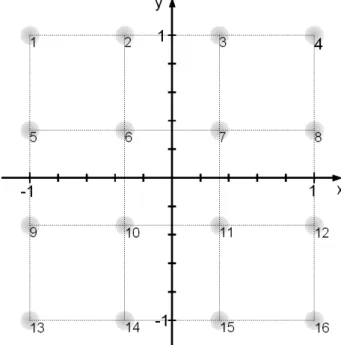
The data acquired using the Hartmann-Shack sensor, is a set of mean deviations in x- directionP_n at the positions (x_n, y_n) of each lensarray and a set of deviations in y-direction at the same location. The values of xand y extend from −1 to 1 and have no dimensions.

The real dimensions can easily be calculated by a multiplication with the real dimensions of the lensarray. An example for a square 4×4 lensarray is shown in figure 5.11.

Figure 5.11: square 4×4-lensarray in coordinate system

(46)

In the 4×4-example we have N = 16 values for the measured derivatives Pn and Qn. P_n = _dx^dW(x_n, y_n)

Q_n = _dy^dW(x_n, y_n) n = 0. . . N (5.3)

For both directions we want to find a function that fits best to the measured values. The estimated wavefront derivatives can be developed in functions L_i(x, y):

d

dxW(x, y) =P

i

k_iL_i(x, y)

d

dyW(x, y) = P

i

l_iL_i(x, y) j = 0. . . J (5.4)

For the optimization of the estimation, a least-square-fit is used.

S_x =

N

X

n=1

d

dxW^∗(x_n, y_n)−P_n 2

=

N

X

n=1

X

i

k_iL_i(x_n, y_n)−P_n

!2

(5.5)

S_y =

N

X

n=1

d

dyW^∗(x_n, y_n)−Q_n 2

=

N

X

n=1

X

i

l_iL_i(x_n, y_n)−P_n

!2

(5.6)

Minimization demands:

0 = dS dk_j = 2

N

X

n=1

X

i

kiLi(xn, yn)−Pn

!

Lj(xn, yn) ∀j (5.7)

0 = dS dl_j = 2

N

X

n=1

X

i

l_iL_i(x_n, y_n)−Q_n

!

L_j(x_n, y_n) ∀j (5.8)

Resolving the braces, we obtain:

N

X

n=1

P_nL_j(x_n, y_n) = X

i

k_i

N

X

n=1

L_i(x_n, y_n)L_j(x_n, y_n) (5.9)

N

X

n=1

Q_nL_j(x_n, y_n) =X

i

l_i

N

X

n=1

L_i(x_n, y_n)L_j(x_n, y_n) (5.10) For both directions we have a set of J equations which should be solved simultaneously.

These calculations can be simplified by using orthogonal functionsL_i(x, y). Orthogonality demands:

N

X

n=1

L_i(x_n, y_n)L_j(x_n, y_n) = 0 ; ∀i6=j (5.11)

(47)

Now we have two sets of J independent equations.

k_j =

N

P

n=1

P_nL_j(x_n, y_n)

N

P

n=1

L²_j(x_n, y_n)

(5.12)

l_j =

N

P

n=1

Q_nL_j(x_n, y_n)

N

P

n=1

L²_j(x_n, y_n)

(5.13)

The set of orthogonal functions L_i used for the following calculations is:

1. Order

L₀ = 1 (5.14)

2. Order L₁ = x

L2 = y (5.15)

3. Order

L3 = 2x y

L₄ = c₁x²+c₁y²−1 L₅ = −x²+y²

(5.16)

3. Order

L6 = c2x y²−x³

L₇ = c₃x³+c₄x y²−2x L₈ = c₃y³+c₄y x²−2y L₉ = y³−c₂y x²

(5.17)

Dissertation submitted to the Combined Faculties for the Natural Sciences and for Mathematics of the Ruperto-Carola University of Heidelberg, Germany for the degree of Doctor of Natural Sciences