NBER WORKING PAPER SERIES
THE GOOD, THE BAD AND THE AVERAGE:
EVIDENCE ON THE SCALE AND NATURE OF ABILITY PEER EFFECTS IN SCHOOLS Victor Lavy
Olmo Silva Felix Weinhardt Working Paper 15600
http://www.nber.org/papers/w15600
NATIONAL BUREAU OF ECONOMIC RESEARCH 1050 Massachusetts Avenue
Cambridge, MA 02138 December 2009
We thank the Center for Economic Performance (CEP) at the London School of Economics (LSE) for seed money for this project. We would also like to thank: Rebecca Allen, Josh Angrist, Kenneth Chay, Steve Gibbons, William R. Johnson, Francis Kramarz, Steve Machin, Michele Pellizzari, Steve Pischke, Steve Rivkin, Yona Rubinstein, Henry Overman, Hongliang (Henry) Zhang, two-anonymous referees and seminar participants at Bocconi University, Brown University, CEP-LSE, CMPO-Bristol University, CREST in Paris, EIEF in Rome, ESSLE 2009, Hebrew University of Jerusalem, IFS and IoE in London, Royal Holloway University, and Tel Aviv University for helpful comments and discussions.
All remaining errors remain our own. The views expressed herein are those of the author(s) and do not necessarily reflect the views of the National Bureau of Economic Research.
NBER working papers are circulated for discussion and comment purposes. They have not been peer- reviewed or been subject to the review by the NBER Board of Directors that accompanies official NBER publications.
© 2009 by Victor Lavy, Olmo Silva, and Felix Weinhardt. All rights reserved. Short sections of text,
not to exceed two paragraphs, may be quoted without explicit permission provided that full credit,
including © notice, is given to the source.
The Good, the Bad and the Average: Evidence on the Scale and Nature of Ability Peer Effects in Schools
Victor Lavy, Olmo Silva, and Felix Weinhardt NBER Working Paper No. 15600
December 2009, Revised May 2011 JEL No. I21,J18,J24
ABSTRACT
In this paper, we study ability peer effects in secondary schools in England and identify which segments of the peer ability distribution drive the impact of peer quality on students achievements. To do so, we use census data for four cohorts of pupils taking their age-14 national tests, and measure students ability by their prior achievements at age-11. We employ a new identification strategy based on within-pupil regressions that exploit variation in achievements across the three compulsory subjects (English, Mathematics and Science) tested both at age-14 and age-11. We find significant and sizeable negative peer effects arising from bad peers at the very bottom of the ability distribution, but little evidence that average peer quality and very good peers significantly affect pupils academic achievements. However, these results mask some significant heterogeneity along the gender dimension, with girls significantly benefiting from the presence of very academically bright peers, and boys marginally losing out.
Victor Lavy
Department of Economics Hebrew University
Mount Scopus Jerusalem 91905 ISRAEL
and Royal Holloway University of London and also NBER
msvictor@mscc.huji.ac.il Olmo Silva
Department of Geography and Environment London School of Economics
Houghton Street London WC2A 2AE
UK http://personal.lse.ac.uk/silvao/
o.silva@lse.ac.uk
Felix Weinhardt
Department of Geography and Environment London School of Economics
Houghton Street
London WC2A 2AE
UK f.j.weinhardt@lse.ac.uk
1. Introduction
The estimation of peer effects in the classroom and at school has received intense attention in recent years. Several studies have presented convincing evidence about race, gender and immigrants‟ peer effects1, but important questions about ability peer effects in schools remain open, with little conclusive evidence.2 In this paper we study ability peer effects in educational outcomes between schoolmates in secondary schools in England. Our aims are both to investigate the size of ability peer effects on the outcomes of secondary school students and to explore which segments of the ability distribution of peers drive the impact of peer quality on pupils‟ achievements. In particular, we study whether the extreme tails of the ability distribution of peers – namely the exceptionally low- and high- achievers – as opposed to the average peer quality drive any significant ability peer effect on the outcomes of other students.
To do so, we use data for all secondary schools in England for four cohorts of age-14 (9th grade) pupils entering secondary school in the academic years 2001/2002 to 2004/2005 and taking their age- 14 national tests in 2003/2004-2006/2007. We link this information to data on pupils‟ prior achievement at age-11, when they took their end-of-primary education national tests, which we exploit to obtain pre-determined measures of peer ability in secondary schools. In particular, we construct measures of average peer quality based on pupils‟ age-11 achievements, as well as proxies for the very high- and very low-achievers, obtained by identifying pupils who are in the highest or lowest 5% of the (cohort-specific) national distribution of cognitive achievement at age-11. The way in which we measure peer ability is a major improvement over previous studies. The majority of previous empirical evidence on ability peer effects in schools comes from studies that examine the effect of average background characteristics, such as parental schooling, race and ethnicity on students‟ outcomes (e.g.
Hoxby, 2000 for the US, and Ammermueller and Pischke, 2009 for several European countries). A limitation of these studies is that they do not directly measure the academic ability of students‟ peers, but rely on socio-economic background characteristics as proxies for this. Additionally, our measures of peer quality are immune to refection problems (Manski, 1993) for two reasons. First, we identify peers‟ quality based on pupils‟ test scores at the end of primary education, before students have to change school and make a compulsory transition to the secondary phase. As a consequence of the large reshuffling of pupils in England during this transition, on average students meet more than 80%
new peers at secondary school, i.e. students that do not come from the same primary. Secondly, we are able to track pupils during this transition, which means that we can single out new peers from old peers, and construct peer quality measures separately for these two groups. In these respects, our strategy follows Gibbons and Telhaj (2008), also on English secondary schools. In our analysis, we
1 See Angrist and Lang (2004) on peer effects through racial integration; Hoxby (2000) and Lavy and Schlosser
(2011) on gender peer effects; and Gould et al. (2009) on the effect of immigrants on native students.
2 Some exceptions are Sacerdote (2001) on ability peer effects among randomly paired roommates in university
housing, and Carrell et al. (2009) on peer effects in squadrons at the US Air Force Academy.
focus on the effect of new peers‟ ability on pupil achievement (controlling for old peers‟ quality), thus by-passing reflection problems.3
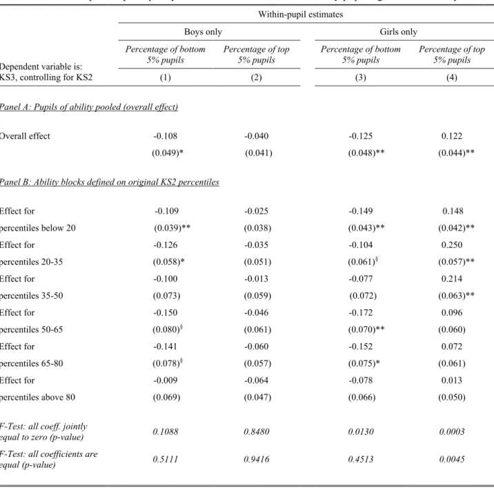
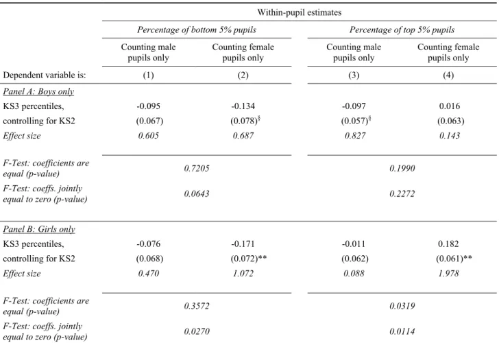
Our results show that a large fraction of „bad‟ peers at school as identified by students in the bottom 5% of the ability distribution negatively and significantly affect the cognitive performance of other schoolmates. Importantly, we find that it is only the very bottom 5% students that (negatively) matter, and not „bad‟ peers in other parts of the ability distribution. On the other hand, we uncover little evidence that the average peer quality and the share of very „good‟ peers as identified by students in the top 5% of the ability distribution affect the educational outcomes of other pupils. However, these findings mask some marked heterogeneity along the gender dimension. Indeed, we show that girls, especially those in the bottom half of the ability distribution, significantly benefit from interactions with very bright peers. In contrast, boys are marginally negatively affected by a larger proportion of academically outstanding peers at school. On the other hand, the negative effect of the very weak students does not significantly vary by the ability of regular students, nor along the gender dimension, and the effect of the average peer quality is estimated to be zero for boys and girls irrespective of their ability. Although we cannot pin down the exact mechanisms that give rise to these effects, we rationalize our findings by drawing on theoretical explanations and related evidence in the economics literature (e.g. Lazear, 2001; Hoxby and Weingarth, 2005; Jackson, 2009), as well as in the psychological and educational research (e.g. Cross and Madson, 1997; Eagly, 1978; Marsh, 2005).
Besides providing some novel insights about the nature of ability peer effects, our paper presents a new identification approach that allows us to improve on the (non-experimental) literature in the field and to identify the effects of peers‟ ability while minimizing biases due to endogenous selection and sorting of pupils, or omitted variables issues. Indeed, the distribution of pupils‟ characteristics in secondary schools in England, like in many other countries, reflects a high degree of sorting by ability.
Using pupils‟ age-11 nationally standardized test scores as an indicator of ability we find that the average ability of peers and a pupil‟s own ability in secondary school are highly correlated. This is so despite the fact that most students have to change school when moving from primary to secondary education and that on average pupils meet more than 80% new peers. Similarly, there is a high correlation between pupils‟ and their peers‟ socioeconomic background characteristics, which is further evidence of sorting. More surprisingly, these correlations survive even when we look at the within-secondary-school variation over time of pupils‟ and their peers‟ ability and characteristic – i.e.
conditional on secondary school fixed-effects.4 This suggests that sorting/selection might be taking place with pupils and schools being affected by and/or responding to cohort-specific unobserved shocks to students‟ and schools‟ quality. Identification strategies that rely on the randomness of peers‟
quality variation within-schools over time find little justification against this background.
3 Note that this does not imply that we are able to separate endogenous from exogenous peer effects (see Manksi, 1993; Moffitt, 2001). We see this as a further and separate issue from reflection problems that arise from previous/simultaneous interactions among students that affect measures of peers‟ ability (Sacerdote, 2001).
4 A similar result is documented by Gibbons and Telhaj (2008) and Black et al. (2009).
In order to overcome this selection problem, we rely on within-pupil regressions – i.e. on specifications including pupil fixed-effects – and exploit variation in achievements across the three compulsory subjects (English, Mathematics and Science) tested at age-14. We further exploit the fact that students were tested on the same three subjects at age-11 at the end of primary schools, so that we can measure peers‟ ability separately by subject. We then study whether subject-to-subject variation in outcomes for the same student is systematically associated with the subject-to-subject variation in peers‟ ability. To the best of our knowledge, we are the first to use pupil fixed-effects and inter-subject differences in achievement to address identification issues of peer effects in schools.
One significant advantage of this approach is that by including pupil fixed-effects we are able to control for pupil own unobservable average ability across the three subjects, as well as for unmeasured family background influences. Additionally, we can partial out in a highly flexible way school-by- cohort fixed-effects and other more general cohort-specific unobserved shocks that might affect pupils‟ outcomes and peers‟ quality similarly across the three subjects. These include unobserved changes in school resources or head teachers, year-on-year variation in the student body‟s composition (e.g. the fraction of pupils from poor family background), as well as changes in the quality of primary schooling or childcare facilities. Given the evidence of year-on-year secondary school sorting highlighted above, controlling for these aspects seems particularly important.
On the other hand, one potential threat to our identification strategy is the possibility that sorting occurs along the lines of subject-specific abilities, so that within-student across-subject variation in ability is correlated with the variation in peers‟ ability across subjects. However, as we shall see below, there is neither a sizeable nor a significant correlation between the within-student across- subject variation in age-11 achievements – i.e. our measure for students‟ subject-specific academic ability – and the variation in peers‟ ability across subjects. Moreover, conditional on pupil fixed- effects, our results are virtually identical irrespective of whether or not we control for pupils‟ own age- 11 test scores. Stated differently, specifications that include pupil fixed-effects effectively take care of the sorting of pupils and their peers into secondary education, and provide reliable causal estimates of ability peer effects. To further support this claim, we provide an extensive battery of robustness checks to our core analysis. These include a set of regressions that focus on a sub-set of pupils with limited school choice from their place of residence, as well as results coming from specifications that further include school-by-subject effects to control for unobservable subject-specific school attributes. This additional evidence lends strong support to the causal interpretation of our results.
The rest of the paper is organized as follows. The next section reviews the literature on peer effects, while Section 3 presents our identification strategy. Section 4 describes the institutional background and our dataset. Section 5 reports our main estimates and robustness checks, while Section 6 presents some heterogeneity in our findings. Finally, Section 7 provides some concluding remarks.
2. Related literature
For a long time social scientists have been interested in understanding and measuring the effects of peers‟ behavior and characteristics on individual outcomes, both empirically (e.g. Coleman, 1966) and theoretically (e.g. Becker, 1974). The basic idea is that group actions or attributes might influence individual decisions and outcomes, such as educational attainment. Despite its intuitiveness, the estimation of peer effects is fraught with difficulties and many of the related identification issues have yet to find a definitive answer. In particular, Manski (1993) highlights the perils of endogenous group selection and the difficulty of distinguishing between contextual and endogenous peer effects. In practice, most studies have ignored this distinction and focused on reduced form estimation as outlined by Moffit (2001). Even then, the literature has had to by-pass a variety of biases that arise because of endogenous sorting or omitted variables and has not yet reached a consensus regarding the size and importance even of these reduced form effects.
Two main issues have taxed researchers interested in the identification of the causal effect of peer quality in education. Firstly, it is widely recognized that a pupil‟s peer group is evidently self-selected and hence the quality of peers is not exogenous to a student‟s own quality and characteristics.5 Failing to control for all observable and unobservable factors that determine individual sorting and achievements would result in biased estimates of peer effects. Secondly, peer effects work in both directions, so that peer achievements are endogenous to one pupils‟ own quality if students have been together for a while. This mechanical issue, known as the „reflection problem‟, is particularly difficult to undo unless the researcher is able to reshuffle group formation and belonging, and measure peers‟
quality in ways that are predetermined to interactions within the group.
To account for these difficulties, recent years have seen a variety of identification strategies.
Different studies have exploited random group assignments (Sacerdote, 2001; Zimmerman, 2003;
Duflo et al., 2008; Carrell et al., 2009; De Giorgi et al., 2009; Gould et al., forthcoming), within- school random variation (Hoxby, 2000; Hanushek et al., 2003; Ammermueller and Pischke, 2009;
Gould et al, 2009; Lavy and Schlosser, 2011), instrumental variables (Goux and Maurin, 2007) or sub- group re-assignments (Katz et al., 2001; Sanbonmatsu et al., 2006).6 Only recently, Lavy et al.
(forthcoming) and Duflo et al. (2008) have tried to enter the „black box‟ of ability peer effects in Israel and Kenya, respectively, and have explicitly focused on understanding the mechanisms through which interactions could exert their effects. Duflo et al. (2008) exploit random assignment of pupils in primary schools in Kenya to classes by ability in order to identify peer effects. The authors find improvements from ability-tracking in primary schools and attribute this result to the fact that more homogeneous groups of students might be taught more effectively. Lavy et al. (forthcoming) present
5 There is a well established literature on the link between school quality and house prices (e.g. Black, 1999;
Gibbons et al., 2009; Kane et al., 2006), suggesting that pupils are segregated into different neighborhoods and schools by socio-economic status.
6 Other examples include Aizer (2008), Bifulco et al. (2008), Burke and Sass (2008), Figlio (2007), Lefgren (2004), Nechyba and Vidgor (2007) and Vidgor and Nechyba (2004).
related evidence of significant negative effects of a high fraction of low ability students in the class on the outcomes of other pupils, which might arise through classroom disruption and decrease in attention paid by the teacher.
The study that is closest to ours in terms of context and data is Gibbons and Telhaj (2008) who also estimate peer effects for pupils in English secondary schools. The authors attempt to control for the endogenous sorting of pupils to secondary schools by allowing for primary and secondary school fixed-effect interactions and trends. However, this approach does not fully eliminate the correlation between pupils‟ own ability and peer quality, and their results provide little evidence of sizeable and significant peer effects.
To the best of our knowledge, our study is the first one to rely on pupil fixed-effects and inter- subject differences in achievement to address identification issues of peer effects in schools. A similar approach has been previously used in Lavy (2009) to investigate the effect of instructional time on academic achievements; Bandiera et al. (2009) to study class size effects at university; and Dee (2007) to study the effect of teacher gender on students‟ attainments. As already mentioned, the within- student approach allows to control for pupil unobservable average ability, unmeasured family background influences, school-by-cohort fixed-effects and other more general cohort-specific shocks that are common to the three subjects. We believe this approach achieves a clean identification of the causal effect of peers‟ ability. The next section spells out in detail our empirical strategy.
3. Empirical strategy
3.1. General identification strategy: within-pupil regressions
The main problem with identifying the effect of the ability composition of peers on pupil educational achievements is that peer quality measures are usually confounded by the effects of unobserved correlated factors that affect students‟ outcomes. This correlation could arise if there is selection and sorting of students across schools based on ability differences, or if there is a relation between average students‟ ability in one school and other characteristics of that school, potentially not fully observed.
The approach commonly used in several recent studies relies on within-school variations in the ability distribution of students across adjacent cohorts or across different classes (e.g. Ammermueller and Pischke, 2009; Hoxby, 2000; Gibbons and Telhaj, 2008; Lavy et al., forthcoming; Lavy and Schlosser, 2011). This method potentially avoids both sources of confounding factors, although the identifying assumption is that the variation of peer quality over time or across classes is idiosyncratic and uncorrelated with students‟ potential outcomes and background.
In this paper, we suggest an alternative approach for overcoming the potential sorting and omitted variable biases, namely we examine subject-to-subject variation in outcomes for the same student and investigate if this is systematically associated with the subject-to-subject variation in peers‟ ability. Stated differently, we study whether pupils who have school peers that have higher
ability in subject j (e.g. Mathematics) than in subject i (e.g. Science), have better cognitive performance in subject j than in subject i.
More formally, using test scores in multiple subjects and four cohorts of 9th graders taking their age-14 national tests in the academic years 2003/2004-2006/2007, we estimate the following pupil fixed-effect equation:
l iqst h qst
qst qst
i q
st q i
iqst Gender P P P
A 1 2 3 (1)
Where i denotes pupils, q denotes subjects (English, Mathematics and Science), s denotes schools and t denotes pupils‟ cohort.
A
iqst is an achievement measure for student i in subject q at school s in cohort t. In our analysis, we focus on test scores in the three compulsory subjects (English, Mathematics and Science) assessed at age-14 during the national tests; these are denoted in England as Key Stage 3 (KS3; more details in Section 4). Additionally, i is a student fixed-effect, q is a subject-specific effect, andst is a school × cohort effect. We also include an interaction term between pupil gender and subject-specific effects which is meant to control for the well-documented gender disparities in achievements in different subjects (see Ellison and Swanson, 2009, and Fryer and Levitt, forthcoming), and their potential effect on pupils‟ sorting into secondary schooling.7 Next,P
qst captures the average ability of peers in subject q in secondary school s in cohort t as measured by test scores in a given subject in the national tests taken by students at age-11 at the end of primary school (denoted as Key Stage 2, or KS2). On the other hand, Pqsth and Pqstl capture the fraction of very high- ability and the very low-ability peers in one students‟ cohort. More precisely, we choose the top and bottom 5% in the (cohort-specific) national distribution of KS2 test scores as the cut off points to determineP
qsth andP
qstl (this cut-off choice is not arbitrary; more details in the data and results sections). Finally,
iqst is an error term that allows for any type of correlation within observations of the same student and of the same school.The coefficients of interest are
1 , which captures the effect of the average ability of peers on students‟ achievement; and
2 and
3, which respectively measure the effect of the proportion of peers in the cohort who are in the top 5% and bottom 5% of the national distribution of KS2 test scores. As discussed above, we are interested in both the absolute and the relative strength and significance of these three coefficients to determine which segments of the peer ability distribution drive any ability peer effect that we will document.Note that one significant advantage of this approach is that pupil fixed-effects „absorb‟ students‟
own unobservable average ability across subjects and unmeasured family background characteristics.
7 We also tried specifications where we interact other pupil characteristics (e.g. eligibility for free school meals) with subject-specific dummies and found virtually identical results. However, we prefer the more parsimonious specification in Equation (1).
Moreover, this specification allows to partial out in a very flexible way school-by-cohort fixed-effects, such as unobserved changes in school resources or head teachers and year-on-year variation in the student body‟s composition (e.g. the proportion of students eligible for free school meals), as well as other cohort-specific unobserved shocks (e.g. changes in the quality of primary schooling or childcare facilities) that affect pupils‟ outcomes and peers‟ quality similarly across the three subjects. This seems particularly important given the issues discussed in Arcidiacono et al. (2009) and the evidence discussed in the Introduction of a significant correlation between pupils‟ characteristics and ability and the characteristics and ability of their peers even conditional on secondary school fixed-effects.
Before moving on, two remarks are worth being made. First, one necessary assumption for our identification strategy is that peer effects are the same for all three subjects; stated differently, we cannot interact the
parameters with
q in Equation (1). Although this restriction does not seem untenable, in the analysis that follows we will provide evidence to support this conjecture. Second, our peer effects are „net‟ measures of peer influences, that is net of ability spillovers across subjects (e.g.peers‟ ability in English might influence pupils‟ test scores in Mathematics). If spillovers are very strong such that subject-specific abilities do not matter, then we are bound to find zero peer effects.
3.2. Dealing with potential threats to identification
Although the strategy described so far allows us to control for pupils‟ average ability across subjects, one concern is the possibility that sorting of students in different schools is partly based on subject- specific ability and considerations. In particular, there might be some residual correlation between the within-student across-subject variation in age-11 prior achievements, capturing students‟ subject- specific abilities, and the variation in peers‟ quality across subjects.
Our first approach to account for such residual sorting is to control for pupils‟ KS2 test scores in the within-pupil estimation. The underlying assumption is that lagged test scores effectively capture any subject-specific abilities and there is no sorting based on unobserved factors that are not correlated with KS2 scores, so that within-subject peer assignment is as good as random conditional on primary school test scores. To our advantage, we can control for lagged test scores in a very flexible way by including in our specification at the same time same-subject lagged test scores (e.g. looking at age-14 English test score for pupil i controlling for age-11 English achievement), as well as cross-subject test scores (e.g. looking at pupil i‟s age-14 English test score controlling for age-11 attainments in Mathematics and Science). This allows to partial out the effect of one pupil‟s own ability in a specific subject, as well as cross-subject effects. Additionally, we can interact lagged test scores with subject- specific dummies, so that age-11 achievements exhibit different effects on age-14 outcomes in different subjects. Under our most flexible and preferred specification, we estimate the following model:
1 h l 1 ( 1) 1 ( 2) 1
iqst i q st q qst qst qst q iqst q iq st q iq st iqst
A GenderP P P a a a (2)
where
a
iqst1 represents same-subject lagged test scores, aiq( 1) st1 anda
iq( 2) st1are the two cross- subjects lagged test scores, and
q,
q and
q are subject-specific parameters that capture the effects of lagged test scores in the same- and cross-subjects.8Anticipating our analysis below, we find that results from within-pupil specifications are virtually identical whether or not we control for pupils‟ own age-11 test scores. This is explained by the fact that – as revealed by the placebo-type test carried out in Table 3 – there is neither a sizeable nor a significant correlation between the within-student across-subject variation in prior achievements, and the variation in peers‟ ability across subjects. Stated differently, conditional on pupil fixed-effects, peers‟ subject-specific quality measures are balanced with respect to pupils‟ own age-11 test scores, and specifications that include pupil fixed-effects effectively take care of the sorting of pupils and their peers into secondary education. Nonetheless, we complement our core strategy with a set of robustness checks to assess the importance of subject-specific sorting. In particular, we restrict our analysis to a sub-set of pupils with limited school choice from their place of residence and for whom concerns about subject-specific considerations are mitigated. Even among these students, our findings hold completely unaffected.
A second source of concern is that, although the pupil fixed-effects strategy accounts for school- by-cohort unobserved shocks, it does not control for subject-specific school unobservables. This raises questions as to whether differences in pupils‟ attainments across subjects are driven by subject- specific differences in their peers‟ quality, or related to other factors such as school specialism in one area of the curriculum or teachers‟ subject-specific abilities.9 In order to minimize these concerns, we exclude from our sample schools with a stated „specialism‟ in a given subject. About 8.5% of secondary school students in England attend a specialist school, and some common areas of specialism include: language; mathematics and computing; science; technology; business and enterprise; and arts.
Additionally, in some of our specifications we include school-by-subject fixed-effects – on top of pupil fixed-effects – to control for subject-specific school unobservables that are persistent over time.
As detailed in the results section, these empirical models are very demanding in terms of the variation they exploit to identify the effects of peers‟ quality. Nevertheless, results from these specifications provide full support to the causal interpretation of our estimates.
3.3. Measuring peers’ ability
A key requirement for our empirical approach is that the proxies of peer ability are based on pre- determined measures of students‟ ability that have not been affected by the quality of his/her peers and do not suffer from reflection problems. The longitudinal structure of the data that we use allows us to
8 Note that conditional on pupil fixed-effects, the same-subject and two cross-subjects lagged test scores cannot be simultaneously identified. Therefore, in our within-pupil empirical specification, we only include the same- subject lagged test score and one of the two cross-subject lagged outcomes.
9 Carrell and West (2010) highlight the importance of teacher quality for university students‟ attainments.
link peers‟ age-11 test scores taken at the end of primary school (6th grade) to students‟ age-14 achievements four years later (9th grade) in secondary school. Additionally, by following individuals over time, we are able to point out which secondary school students come from the same primary and identify who the new peers and the old peers are. In the national sample, on average 87% of pupil i‟s peers at secondary school did not attend the same primary institution as student i, and therefore their age-11 test scores could not have been affected by this pupil. Following Gibbons and Telhaj (2008), in our analysis, we construct peer quality measures separately for new peers and old peers, and focus on the effect of new peers on pupil achievement. Nevertheless, we include measures of the quality of old peers in our empirical specifications to control for primary-school × cohort × subject effects that might persist on age-14 test scores and that are shared by pupils coming from the same primary school and cohort. Note that our estimates are not sensitive to the inclusion of these variables.
Two additional remarks are worth being made. First, we use information about the school that a pupil is attending at age-12 (7th grade), when he/she enters secondary education, to define our base population. Similarly our three measures of peer quality „treatment‟ (the „good‟, the „bad‟ and the average peer quality) are based on 7th-grade enrollment. This is because any later definition of these proxies, for example as recorded at age 14, might be endogenous.
Second, in implementing this methodology, we use peers‟ ability measured at the grade and not at the class level because our data does not include class identifiers. We do not see this as a particularly restrictive compromise since the majority of schools do not strictly group pupils with different subject-specific abilities into different classes at the early stages of secondary education (more details in the next section). Therefore, the quality of peers within a grade is likely to be strongly correlated with the quality of peers within classes. However, if a significant degree of subject-specific tracking takes place, grade-level peer quality measures might capture the peer quality actually experienced by pupils with some noise, thus leading to downward-biased estimates of the effect of peers‟ ability.10 To minimize these issues, our main analysis focuses on the 50% smallest secondary schools in England, with a maximum grade-7 cohort-size of 180 students, and 135 7th grade-students on average. Small schools will have fewer classes since they receive funding based on pupil numbers and have clear incentives to run classes at maximum capacity (approximately 30/35 students). This implies that students will be more mixed with peers of heterogeneous abilities in small schools than in larger ones, where more classes can be created to group students according to their abilities. However, to further assess the importance of these issues, we will investigate whether our results change when we focus on a sub-set of even smaller secondary schools (average cohort size 120), as opposed to all schools in England irrespective of their size.
10 Note however that even having access to information about class identifiers would not solve this issue if students can choose their networks – and thus their peers – within classes or outside of these. On the other hand, our study does not suffer from measurement error due to incomplete information on pupils‟ schoolmates as in Ammermueller and Pischke (2009).
4. Institutions, data and descriptive statistics 4.1. Schooling in England: institutional background
Compulsory education in England is organized into five stages referred to as Key Stages. In the primary phase, pupils enter school at age 4-5 in the Foundation Stage, then move on to Key Stage 1 (KS1), spanning ages 5-6 and 6-7 (corresponding to 1st and 2nd grade in the US educational system).
At age 7-8 pupils move to KS2, sometimes – but not usually – with a change of school. At the end of KS2, when they are 10-11 (6th grade), children leave the primary phase and go on to secondary school where they progress through KS3 (7th to 9th grade) and KS4 (10th to 12th grade). Importantly, the vast majority of pupils have to change schools on transition from primary to secondary education, and move on to the school of their choice.
Indeed, since the Education Reform Act of 1988, the „choice model‟ of school provision has been progressively extended in the state-school system in England (Glennerster, 1991). In this setting, pupils can attend any under-subscribed school regardless of where they live and parental preference is the deciding factor. All Local Education Authorities (LEAs) and schools must organize their admissions arrangements in accordance with the current statutory Governmental Admissions Code of Practice. The guiding principle of this document is that parental choice should be the first consideration when ranking applications to schools. However, if the number of applicants exceeds the number of available places, other criteria which are not discriminatory, do not involve selection by ability and can be clearly assessed by parents, can be used to prioritize applicants. These vary in detail, but preference is usually given first to children with special educational needs, next to children with siblings in the school and to those children who live closest. For Faith schools, regular attendance at designated churches or other expressions of religious commitment is foremost. As a result, although choice is the guiding principle that schools should use to rank applications, it has long been suspected that schools have some leeway to pursue some forms of covert selection based on parental and pupil characteristics that are correlated with pupil ability (see West and Hind, 2003).
As for testing, at the end of each Key Stage, generally in May, pupils are assessed on the basis of standard national tests (SATS), and progress through the phases is measured in terms of Key Stage Levels, ranging between W („Working towards Level 1‟) up to Level 5+ during primary education and Level 7 at KS3. Importantly, at both KS2 and KS3 students are tested in three core subjects, namely Mathematics, Science and English, and their attainments are recorded in terms of the raw test scores, spanning the range 0-100, from which the Key Stage Levels are derived. We will use these test scores to measure pupils‟ attainments at KS3 and identify peers‟ quality as measured by their KS2.
Finally, regarding the organization of teaching and class formation, two important issues are worth mentioning. First, the notion of „class‟ is a rather hollow one in English secondary schools since students are grouped with different pupils for different subjects. A second important aspect that – at least nominally – characterizes English secondary education is the practice of „ability setting‟, i.e.
subject-specific tracking. Under these arrangements, secondary school pupils are initially taught in
mixed-ability groups for an observation and acclimatization period of around a year, and then eventually educated in different groups for different subjects according to their aptitude in that topic.11 However, despite some support from the central Government, the practice of ability setting is not liked nor supported by teachers, and as a result has not been fully adopted by secondary schools. Data collected by the Office for Standards in Education (OFSTED) in 2001-2002 from inspection of 566 secondary schools (cited in Kutnick et al., 2006) shows that only about 26% of these had subject- specific setting from 7th grade, with the percentage increasing to around 40% in 9th grade. Further evidence is provided by Kutnick et al. (2006), who gathered data for a small set of medium-to-large sized secondary schools with on average around 200 students in grade 7. This study shows that only around 50% of the schools had ability sets for Mathematics from 7th grade, with the figures being substantially lower for English and Science, respectively at 34% and 44%. Although these numbers increase as students reach 9th grade, subject-specific setting remains far from universal, with the figures being 46%, 59% and 80% in English, Science and Mathematics respectively. In conclusion, two features emerge from this discussion. First, because of the lack of clearly defined and stable classes during secondary education, students will predominantly interact with different peers in different subjects. Second, since ability setting is not strictly implemented, pupils will face a variety of class-mates with a heterogeneous range of abilities during instruction time even for the same subject.
Finally, recall that our analysis focuses on the 50% smallest secondary schools in England – with on average 65 pupils (i.e. two classes) less than those sampled by Kutnick et al. (2006). This further minimizing issues due to subject-specific ability setting.
4.2. Data construction
The UK‟s Department for Children, Schools and Families (DCSF) collects a variety of data on all pupils and all schools in state education.12 This is because the pupil assessment system is used to publish school performance tables and information on pupil numbers and pupil/school characteristics is necessary for administrative purposes – in particular to determine funding. Starting from 1996, a database exists holding information on each pupil‟s assessment record in the Key Stage SATS described above throughout their school career. Additionally, from 2002 the DCSF has carried out the Pupil Level Annual School Census (PLASC), which records information on pupil‟s gender, age, ethnicity, language skills, any special educational needs or disabilities, entitlement to free school meals and various other pieces of information, including the identity of the school attended during years other than those when pupils sit for their Key Stage tests. PLASC is integrated with the pupil‟s assessment records in the National Pupil Database (NPD), giving a large and detailed dataset on pupil
11 Subject-specific ability is often gauged using end-of-primary education KS2 test scores. However, these are only available to schools several months after they have admitted pupils and teachers have some discretion in determining the ability set that is most appropriate for their students in different subjects (see DfES, 2006).
12 The private sector has a market share of about 6-7%. However, very little consistent information exists for pupils and schools in the private domain. For this reason, we do not consider private schooling in our analysis.
characteristics, along with their test histories. Furthermore, various other data sources can be merged in at school level using the DCSF Edubase and Annual School Census, which contain details on school institutional characteristics (e.g. religious affiliation), demographics of the students (e.g.
fractions of pupils eligible for free school meals) and size (e.g. number of pupils on roll).
The length of the time series in the data means that it is possible to follow the academic careers of four cohorts of children from age-11 (6th grade) through to age-14 (9th grade), and to join this information to PLASC data for every year of secondary schooling (7th to 9th grade). The four cohorts that we use include pupils who finished primary education in the academic years 2000/2001 to 2003/2004, entered secondary school in 2001/2002 to 2004/2005, and sat for their KS3 exams in 2003/2004 to 2006/2007. We use information on these four cohorts because this is the only time- window where we can identify the secondary school where pupils start their secondary education and not only the one where they take their KS3 tests. This is crucial to our analysis since we want to measure peer exposure at the beginning of secondary schooling (in 7th grade), and not after three years (in 9th grade). The data also allows us to gather information about the primary schools where pupils took the KS2 exams, which implies that we are able to single-out secondary schoolmates that are new peers from those who instead came from the same primary school (i.e. old peers).
Using this set of information we construct a variety of peer quality measures based on pupil achievements at KS2 in the three core subjects. In order to do so, we use the KS2 test scores, separately by subject and cohort, to assign each pupil to a percentile in the cohort-specific and subject- specific national distribution. We then go on to create three separate measures of peer quality. First, we compute the average attainments of peers in the grade at school. Next, we create two measures that capture peer effects coming from the „very best‟ and the „very worst‟ students at school, namely the fraction of peers in the grade below the 5th percentile or above the 95th percentile of the cohort-specific national distribution of KS2 test scores.
We have imposed a set of restrictions on our data in order to obtain a balanced panel of pupil information in a balanced panel of schools. First, we have selected only pupils with valid information on their KS2 and KS3 tests for whom we can also match individual background characteristics and the identity of the school where they start their secondary education using PLSAC. Given the quality of our data, this implies that we drop less than 2.5% of our initial data. Next, we have focused on schools that are open in every year of our analysis, and have further dropped secondary schools that have a year-on-year change of entry-cohort size of more than 75% or enrolments below 15 pupils. While the former restriction excludes schools that were exposed to large shocks that might confound our analysis, the latter excludes schools that are either extremely small or had many missing observations.
These restrictions imply that we lose less than 2.5% of our initial observations. We have also excluded selective schools (e.g. Grammar schools) from our analysis, as these can actively choose their pupils based on their ability (about 8% of our original sample). Furthermore, we drop schools where the fractions of pupils below the 5th percentile or above the 95th percentile of the cohort-specific KS2
national distribution do not exhibit any variation over the four years under analysis. These restrictions predominantly trim schools that have no students in either the top or bottom 5% of the ability distribution in any year in any subject, and would thus not contribute to the identification of peer effects. Since these constraints imply that we drop about 10% of the sample, we checked that our main results are not affected when we omit these restrictions. Finally, we focus on the 50% smallest secondary schools in England, with a maximum 7th grade cohort-size of 180 students, and 135 grade-7 students on average. Our final dataset includes a balanced panel of approximately 500,000 pupils for whom we can observe complete information in terms of KS2 and KS3 test scores, individual and family background characteristics, and both primary and secondary school level information from age- 11 to age-14. In the next section, we present some descriptive statistics.
4.3. Some descriptive statistics
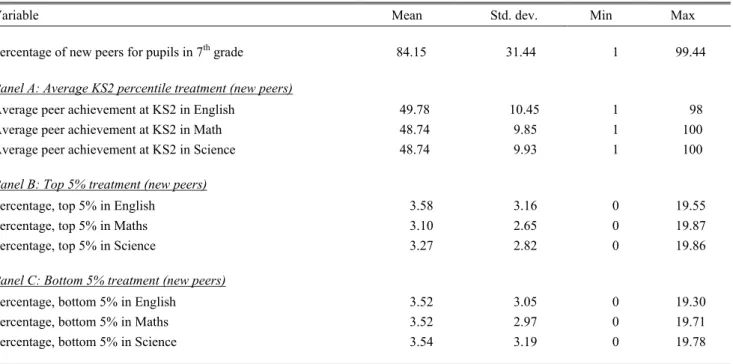
In Column (1) of Table 1 we present descriptive statistics for the main variables of interest for the sample of „regular‟ students, defined as the set of pupils with age-11 test scores in the three subjects above the 5th percentile and below the 95th percentile of KS2 test score distribution. In the same table, we also presents descriptive statistics for pupils in either the top 5% or bottom 5% tails of the ability distribution – which we also label as „treatments‟. The regression analysis that follows is mostly based on the sample that includes all students, i.e. „regular‟ pupils and the „treatments‟. However, we will also discuss some results based on the sample that excludes the top and bottom 5% pupils to keep the distinction between treated students and pupils that form our treatments clean.
In the top panel of the table we describe pupils‟ test scores at KS2 and KS3. Unsurprisingly, the first column shows that test score percentiles of regular students are centered just below 50, for all subjects and at both Key Stages. The correlations of pupils‟ KS2 test scores across subjects are 0.59 for English and Mathematics; 0.62 for English and Science; and 0.68 for Science and Mathematics. At KS3 these correlations increase to 0.64, 0.68 and 0.80, respectively. Appendix Table 1 further shows that the within-pupil variations of KS2 and KS3 test scores across the three subjects are respectively 11.8 and 10.9. This provides evidence that test scores are not perfectly correlated across subjects for the same student, although they tend to be more closely associated in Science and Mathematics, in particular at KS3.
The remaining two columns of the table illustrate how pupils with at least one subject in either the top 5% or the bottom 5% of the ability distributions score at their KS2 and KS3 tests. By construction, pupils in top 5% of the KS2 test score distribution perform much better than any other pupil in their KS2 exams, while the opposite is true for pupils in the bottom 5% tail. We get a very similar picture if we look at pupils‟ KS2 test scores in one subject (e.g. English) imposing that at least one of the other two subjects (e.g. Mathematics or Science) is above the 95th percentile or below the 5th percentile of the test score distribution. More interestingly, this stark ranking is not changed when we look at KS3 test scores, for all subjects, with little evidence of significant mean reversion in the achievements of very good and very bad peers between age-11 and age-14. To further substantiate this
point, we have analyzed the KS3 percentile ranking of pupils in the top and bottom 5% of the KS2 achievement distribution. For all subjects, about 80% of the pupils ranking in the bottom 5% at KS2, still rank in the bottom 20% of the KS3 distribution, with approximately 70% of them concentrated in the bottom 10%. At the opposite extreme, around 80% of pupils ranking in the top 5% at KS2 remains in the top 20% of the KS3 achievement distribution, with the vast majority still scoring in the top 10%.
In a nutshell, our „good‟ and „bad‟ peers are persistently among the brightest and worst performers.
The second panel of Table 1 presents more information on pupil background characteristics. The figures in the first column reveal that the „regular‟ sample is representative of the population of English secondary school pupils. On the other hand, pupils with at least one subject in the bottom 5%
are less likely to have English as their first language and more likely to be eligible for free school meals (a proxy for family income). The opposite is true for pupils with at least one subject in the top 5%. However, the differences in family background are much less evident than those in terms of academic ability presented in Panel A. Peer ability measures defined in terms of pupil background would therefore severely underestimate differences in peers‟ academic quality.13
Finally, in Panel C we describe some school characteristics for the various sub-groups. Around 63% of all pupils attend Community schools, while about 25% of the pupils attend a religiously affiliated state-school. This figure is higher than in the national data (at around 16%), because religious schools tend to be of the smaller type that we sample here. Pupils with at least one subject in the top 5% of the ability distribution are less likely to attend a Community school, and more likely to be in a faith school, than pupils in the central part of the ability distribution and students with at least one subject in the bottom 5%. However, these differences are not remarkable.
In Table 2, we present some descriptive statistics of our „treatments‟ for the new peers only. The top figures show that the median share of new schoolmates is 84%, although the distribution of new peers at school is right-skewed, with many more pupils facing almost 100% new schoolmates than at most 1%. The 25th and 75th percentiles of the distribution of new peers are 67% and 94%, respectively.
Next, Panel A summarizes average peer quality (by-construction close to fifty for all subjects), whereas Panels B and C present descriptive statistics for our proxies for „good‟ and „bad‟ peers. Note that all peer quality measures display quite a wide range of variation, although this mainly captures differences across schools. Nevertheless, Appendix Table 1 shows that the same pupil faces considerably different fractions of academically bright and weak students across different subjects, as well as a significant amount of within-pupil across-subject dispersion in average peer‟s age-11 test scores. This is the variation that our pupil fixed-effect regressions exploit to identify the effect of peer quality. Finally, note that the incidence of pupils with at least one subject in the top 5% or the bottom
13 Note that pupils in the bottom 5% of the KS2 distribution are more likely to change school between 7th and 9th grade. Additional results (not tabulated) also show that „regular‟ students are less likely to change school during this period if they face more „good‟ peers as well as more „bad‟ peers. This advocates our use of peer quality measures based on schools attended in 7th grade. On the other hand, we are not concerned with the overall effect of school mobility on pupil achievements as this is controlled for in our pupil fixed-effect strategy.
5% of the KS2 distribution is not concentrated in just a handful of schools: only four schools in our sample do not have at least some „good‟ and some „bad‟ peers in a given year. Moreover, the median, 10th and 90th percentiles of the school-by-year distribution of the percentage of very bright and very poor peers are respectively: 9.7%, 3.9% and 17.3%; and 7.3%, 2.6% and 15.1%.
5. Results
5.1. Effects of peers’ ability: main findings
We begin the discussion of our results by presenting estimates of the impact of the peer quality on pupil outcomes at KS3 and controlling for any potential subject-specific sorting by including lagged test scores as discussed in Section 3.2. Results are reported in Panel A of Table 3. Columns (1) and (2) present OLS and within-pupil estimates of the effect of average peer quality. Columns (3) and (4) present OLS and within-pupil estimates of the effect of the percentage of bottom 5% peers, while Columns (5) and (6) present estimates of the effect of the percentage of top 5% peers. These estimates come from a variety of specifications, which differ in the way they control for lagged test scores. In the first two rows, we report estimates unconditional on age-11 achievements, while the third row presents estimates where we include pupils‟ own KS2 attainment in the same subject in interaction with subject dummies. Finally, in the last row of Panel A, we include pupils‟ own KS2 test scores in the same-subject and cross-subject in interaction with subject effects. Note that the results in the first row are obtained from different regressions, where only one of the three peer quality measures is used as treatment. Results in the remaining rows instead come from regressions that include all treatments together. Finally, standard errors are clustered at the school level to allow for any degree of correlation in pupils‟ residuals across subjects, within schools and over cohorts.
Starting from the first two rows, OLS estimates in Column (1) show a high and positive partial correlation between average peer quality and students‟ KS3 achievements. The estimated coefficient is approximately 0.30 when only the average peer quality is entered in the regression, and drops to 0.12 when the quality of top and bottom peers is further appended to the specification. This suggests that the tails of the ability distribution capture most of the relation between average peer ability and KS3 achievements.14 A similar picture emerges when looking at Columns (3) and (5), which display OLS estimates of the effect of top 5% and bottom 5% peers at schools: the estimated coefficient on „good‟
peers is large – between 0.83 and 0.46 – while the estimated association with „bad‟ peers is significantly negative and in the order of -0.8/-1.1.
A markedly different picture emerges when looking at Columns (2), (4) and (6), where we report results from specifications that include pupil fixed-effects. Column (2) shows that the positive impact of average peer quality completely disappears upon inclusion of pupil fixed-effects. This is now estimated to be at most 0.01, and not statistically different from zero. Similarly, Column (6) shows that
14 To avoid double counting, we have also computed and experimented with measures of the average peer quality that exclude the top 5% and bottom 5% tails, and have come to similar conclusions.
the within-pupil estimates of the effect of the most academically talented peers are positive, but small and not statistically different from zero. Only the effect of the bottom 5% peers remains sizeable and significantly negative after including pupil fixed-effects. As shown in Column (4), this is estimated to be -0.135 in the first row, and -0.124 in the second row, where all three treatments are included simultaneously. Focusing on the latter, this is approximately one sixth of the corresponding OLS estimate. Although one reason why within-pupil estimates of peer effects might be smaller than OLS is because they net out overall effects that might arise through cross-subject interactions, this dramatic reduction is more likely due to the fact that within-pupil estimates control for pupil own unobserved average ability, unmeasured background characteristics and school-by-cohort unobserved effects.
In the last two rows of Panel A of Table 3, we present estimates from specifications where we include lagged test scores as a way to control for any residual pupil subject-specific ability and sorting.
Comparing the second row to the third and fourth, we find that the OLS estimates of ability peer effects are now between 10% and 50% smaller than before. However, even when controlling for lagged test scores in the OLS specification in a very flexible way as in Row (4), we are unable to reduce our estimates of the effect of peers‟ quality to values close to the within-pupil estimates. This strongly speaks in favor of pupil fixed-effects regressions. On the other hand, the within-pupil estimates are essentially unaffected by the inclusion of pupils‟ age-11 test scores. The effect of the average peer quality remains small and insignificant, while the effect of the share of bright students increases from around 0.02 to approximately 0.04, but remains clearly insignificant. More interestingly, the effect of the bottom 5% peers only marginally drops to -0.120 from -0.124, when we include KS2 attainment.15,16 This finding is particularly reassuring especially considering that the same-subject lagged test score enters the within-pupil regressions with a large coefficient (of about 0.35 for example in the third row), and is highly significant.
In fact, the reason why the inclusion of lagged test scores hardly affects the within-pupil estimates of effect of peer quality is that there is neither a sizeable nor a significant correlation between the within-student across-subject variation in own age-11 achievements and the variation in peers‟ ability across subjects. Stated differently, conditional on pupil fixed-effects, peer quality in one subject is balanced with respect to pupils‟ own age-11 test scores in that subject. We show this formally in Panel B of Table 3, where we present results from regressions of one pupil‟s own age-11 test scores on the three peer quality measures (controlling for subject and subject-by-gender dummies).
We label this regression analysis a „placebo-type‟ test since we expect to find no relation if the
15 We have also tried some specifications where we further include age-7 test scores. These are available for only three out of out four cohorts, Moreover, students are not tested in science at age 7 and we had to impute test scores in this subject using the average between mathematics and English. Even then, our findings were fully confirmed, with no effects coming from average peer quality and top students, and strong negative (same size) effects from the fraction of bottom 5% peers.
16 Note that the negative effect of „bad‟ peers is slightly larger if we focus on students with a very high percentage of new peers at school. For example, considering the sample of pupils with at least 97% new peers (corresponding to the 10% percent of students with the largest fraction of new peers) we still find that only the fraction of bad peers has a significant impact, now estimated to be at -0.133 (s.e. 0.046).
variation in our „treatments‟ is as good as random conditional on pupil fixed-effects. Columns (1), (3) and (5) present OLS estimates, whereas Columns (2), (4) and (6) come from the within-pupil specification detailed in Equation (1). OLS results show that unconditional on pupil fixed-effects there is a large and significant degree of sorting. For example, the association between pupils‟ own age-11 test scores and the fraction of bottom 5% peers is -0.40 and strongly significant. However, when we include pupil fixed-effects this relation drops by a factor of twenty to -0.021 (with a standard error of 0.017), and is not significant at conventional levels. Similarly, the within-pupil estimate in Column (2) shows that there is no significant relation between students‟ prior achievement in a given subject and the average peer quality in that subject. The estimated effect is as small as 0.012 and not statistically significant. Finally, the OLS estimate for the fraction of top 5% peers is 0.391 with a small standard error (0.017), suggesting large positive sorting. However, adding pupil fixed-effects eliminates this relation and reverses the sign of the placebo-test estimate to -0.034. Even though this coefficient is marginally significant, we regard it as spurious correlation. In fact, as we noted above, the estimated effect of the top 5% peers is not significantly changed when adding lagged test scores as controls. All in all, these findings suggest that within-pupil specifications effectively take care of the endogenous sorting of pupils and their peers into secondary education, and that any residual subject-specific sorting is too small to confound out estimates.
Before moving on, note that the results so far come from regressions that include the top 5% and bottom 5% peers in the sample that we use to estimate the peer effects. However, as discussed above, an alternative would be to exclude the „good‟ and „bad‟ peers from the estimation sample in order to keep the distinction between treated pupils (i.e. the „regular‟ students of Table 1) and „treatments‟
clean. If we follow this approach, we find very similar results: our estimates of the effect of average peer quality and the top 5% peer are both small and insignificant at 0.000 (s.e. 0.014) and 0.054 (s.e.
0.040), respectively. On the other hand, the effect of the bottom 5% peers is a significant -0.128 (s.e.
0.047), slightly larger than our baseline estimate in Row (4), Panel A, Table 3.17 5.2 Robustness to potential threats to identification
In this section, we present a set of robustness checks that support the causal interpretation of our findings. Results are presented in Panel A of Table 4. Estimates come from within-pupil specifications that control for same- and cross-subject KS2 test scores interacted with subject specific dummies as described by Equation (2). Further details are provided in the note to the table.
As discussed in Section 4, parental choice is the guiding principle that education authorities should adopt when ranking pupils‟ applications to schools. However, when schools are over- subscribed, they have some discretion in prioritizing pupils for admissions and once concern is that
17 Regarding the effect of average peer quality being zero, we further looked into this issue by using the specification of Row (4), but including in the regression only the average peer quality variable. When doing this, the within-pupil estimates goes from 0.002 to 0.012 (but remains insignificant). This suggests that the reason why average peer quality does not have a sizeable impact when we include proxies for peers in the ability tails is that these capture most of the relevant „empirical action‟, and not because we estimate net peer effects.
they might covertly select students with characteristics that are particularly suited to their teaching expertise and other infrastructures specific to one of the three core subjects under analysis. Note that we are not concerned with potential selection based on pupil overall ability, as this is fully taken care of in the within-pupil specifications. To allay these concerns, Row (1) in Panel A of Table 4 presents results obtained by excluding over-subscribed schools (accounting for approximately 35% of the pupils in our baseline sample). The estimates of the effects of peers‟ ability are similar to those obtained before, in particular for the impact of the fraction of bottom 5% peers, which is now slightly larger at -0.131 (s.e. 0.048). Further results (not tabulated, but available upon requests) also show that our findings are similar for secular schools and schools with a religious affiliation. All in all, this suggests that neither school-side selection of pupils with unobservables potentially correlated with ability in a given subject, nor other school institutional features drive our main results.
A second robustness check assesses whether parental choice of schools with an „expertise‟ in a given subject might confound our estimates. To do so, we examine whether our findings are driven by sorting of students who attend a school with peers that excel in the same subject. More precisely, we identify two groups of students: (i) those who excel in subject q (say English) and go to schools where, on average over the four years of our analysis, new peers also excel in that subject; and (ii) those who excel in subject q (say, again, English) and go to schools where, on average, new peers excel in a different subject (either Mathematics or Science). We label these two groups as „sorted‟ and „mixed‟
pupils, respectively.18 We then re-run our analysis including only „mixed‟ students to understand whether our results are driven by sorting of pupils with unobservables that are conducive to excellence in subject q (e.g. English) in the same school. Results from this exercise are reported in Row (2) of Panel A of the table and support our previous findings. Even when considering only „mixed‟ pupils, we find no significant effects from peers of average quality and the fraction of new peers in the top 5%
of the ability distribution. On the other hand, we still find a sizeable and statistically significant negative effect from the bottom 5% peers. The estimated impact is -0.120 (s.e. 0.046), which fully confirms our results so far.
To further assess the robustness of our findings against the possibility of subject-specific sorting, we perform two additional validity checks based on focusing on a subset of students with restricted
„school choice‟. To carry out the first exercise, we exploit detailed geographical information on pupils‟ place of residence and location of the schools they attend, namely geo-coded postcodes with one- meter-precision geographical coordinates. Using this data, we start by calculating for each postcode of residence the median distance that pupils living in that postcode travel in order to attend their school.
In our sample, this median home-school travel distance is on average 3km (or 1.9miles). For every pupil, we then count the number of schools other than the one currently attended that are within the median home-school travel distance for the postcode where he/she lives. We label this set of schools
18 Note that peers‟ excellence in a subject is defined using new peers‟ average KS2 test scores. Our results are unaffected if we use the fraction of new peers in the top 5% of the ability distribution.