MatthiasChristophBernhardPaulsenFebruary2017Advisor:Prof.Dr.WernerBley Computationof ( S,T ) -units Bachelor’sthesis

Ludwig-Maximilians-Universität München Fakultät für Mathematik, Informatik und Statistik

Mathematisches Institut

Bachelor’s thesis

Computation of (S, T )-units

Matthias Christoph Bernhard Paulsen February 2017

Advisor: Prof. Dr. Werner Bley

Recent conjectures in algebraic number theory like the Rubin Stark conjecture rely on

(S, T )-units, which are a subgroup of the S-units of an algebraic number field. In this

thesis, a practical algorithm for the computation of (S, T )-units will be developed and an

implementation in the computational algebra system Magma will be given. Furthermore,

the connection to the (S, T )-class group will be revealed and will be used to verify the

results of the algorithm.

1 Introduction 5

2 From units to S-units 8

2.1 Unit and class group computation . . . . 8

2.2 Definition of S-units . . . . 11

2.3 Computation of S-units . . . . 12

2.4 The S-class group . . . . 13

3 From S-units to (S, T )-units 15 3.1 Idea and Definition . . . . 15

3.2 Computation of (S, T )-units . . . . 16

3.3 Implementation within Magma . . . . 18

3.4 The (S, T )-class group . . . . 20

3.5 Computation of the (S, T )-class group . . . . 22

3.6 Heuristic verification . . . . 23

4 Examples 25

List of symbols 28

Source code of STClassGroup 30

Bibliography 33

1 Introduction

Throughout this thesis, we fix an algebraic number field K. We denote by O

its ring of integers and by O

the group of units in O

. In general, O

is not a unique factorization domain. This motivates the passage from integers to ideals. Let P

be the set of prime ideals

in O

. Because O

is a Dedekind domain, every ideal 0 6= a C O

has a unique decomposition

a =

p∈PK

p

, e

∈ N

with e

= 0 for almost all p ∈ P

. In this sense, ideals and prime ideals generalize the usual integers and prime numbers naturally.

Ideals (except the zero ideal) are just a special case of fractional ideals, i. e. finitely generated non-zero O

-submodules of K. The set I

of fractional ideals in K forms a group, where the inverse of a ∈ I

is given by

a

= {x ∈ K | xa C O

} . Every fractional ideal a ∈ I

has a unique decomposition

a =

p∈P_K

p

, e

∈ Z

with e

= 0 for almost all p ∈ P

. Therefore, I

can be considered as the free abelian group over P

.

Each prime ideal p ∈ P

defines a discrete valuation v

: K

→ Z where v

(α) = e

is the exponent of p in the prime decomposition of αO

. For convenience, let v

(0) = ∞.

It follows that

O

= {α ∈ K | v

(α) ≥ 0, p ∈ P

} O

= {α ∈ K | v

(α) = 0, p ∈ P

} .

As usual, we define the norm of an ideal 0 6= a C O

via N (a) := |O

/a|. The multiplication by an element α ∈ K constitutes a Q -linear map K → K, the determinant of which is called the norm N

(α). For an algebraic integer, the element norm coincides with the norm of the corresponding principal ideal, i. e. N

(a) = N (aO

) for all 0 6= a ∈ O

.

1In this context, the zero ideal is not considered as a prime ideal. So in fact,PK is the set of maximal ideals inOK.

If ν denotes the degree of the extension K | Q , K possesses ν distinct embeddings into C . These split into r real embeddings σ

, . . . , σ

and t pairs of (proper) complex embeddings τ

, τ

, . . . , τ

, τ

, where ν = r + 2t. These embeddings give rise to r + t archimedian valuations on K via |α|

:= |σ

(α)| for i ∈ {1, . . . , r} and |α|

:= |τ

(α)|

for i ∈ {1, . . . , t}.

While the unit group O

is the kernel of the transition K

→ I

α 7→ αO

from non-zero field elements to fractional ideals, the class group Cl

:= I

/H

is defined as its cokernel, where

H

:= {αO

| α ∈ K

} ≤ I

is the subgroup of principal fractional ideals. Then we have the exact sequence 1 → O

→ K

→ I

→ Cl

→ 1 .

Therefore, the determination of O

and Cl

are of special interest.

One of the main results in classical algebraic number theory is that the class group Cl

is always finite. Its cardinality h

:= |Cl

| is called the class number of K. One could say that h

measures the “failure” of O

being a principal ideal domain. In particular, h

= 1 is equivalent to O

being a principal ideal domain.

Another main result is the Dirichlet unit theorem, which states that the unit group O

has finite rank, namely r + t − 1. The torsion part of O

consists exactly of the roots of unity inside K and is therefore finite cyclic. In other words, there exist so called fundamental units ε

, . . . , ε

∈ O

such that

O

= ε

× ε

× · · · × ε

where ε

is a primitive w

-th root of unity. This means that every unit ε ∈ O

has a unique representation ε = ε

· · · ε

with f

, . . . , f

∈ Z and 0 ≤ f

< w

. It turns out that the determination of ε

and w

is rather straightforward. On the other hand, the efficient computation of the fundamental units ε

, . . . , ε

requires a lot harder work and is still subject to current research. In Section 2.1, a brief overview will be given on how to attempt this problem, together with an approach for the computation of Cl

. Associated to K is its Dedekind zeta function

ζ

(s) :=

06=aCOK

1

N (a)

=

p∈PK

1 − 1 N (p)

−1

that generalizes the Riemann zeta function obtained for K = Q . It can be shown [Neu92]

that the defining series of ζ

(s) converges absolutely and uniformely on Re(s) ≥ 1 + δ

for all δ > 0, and that ζ

has an analytic continuation on C \ {1}. By the analytic class number formula, the residuum of ζ

(s) at s = 1 equals

s→1

lim (s − 1)ζ

(s) = 2

π

h

R

w

|d

|

,

where R

is the regulator of K and d

is its discriminant. This is a surprising and beautiful connection between analytic properties of the holomorphic function ζ

and algebraic invariants of the number field K.

Because the constants w

and d

can be computed rather easily, the analytic class number formula discloses information about the product h

R

. While the class number h

is strongly related to the class group Cl

, the regulator R

is connected to the unit group O

. Hence, the knowledge of h

R

comes in handy when computing Cl

and O

simultaneously.

Given a finite set S ⊂ P

of prime ideals in O

, we can generalize integers and units to S-integers and S-units in the following way:

O

:= {α ∈ K | v

(α) ≥ 0, p ∈ P

\ S}

O

:= {α ∈ K | v

(α) = 0, p ∈ P

\ S}

Then O

is the localization of O

by a suitable multiplicative set, as we will see later in Section 2.2.

The (S, T )-units O

are a subgroup of O

depending on a further finite set T ⊂ P

of prime ideals which is disjoint from S. They play an important role in the Rubin Stark conjecture [Rub96] that was formulated by Karl Rubin in 1996. The precise definition of O

will be given in Section 3.1. As far as the author knows, the computation of (S, T )-units is not yet available in computational algebra systems like Magma or Pari.

Therefore, this thesis aims to develop and implement an algorithm for the calculation of

O

, which will be done in the Sections 3.2 and 3.3.

In this chapter, we will first recall a known algorithm for combined computation of the unit and class group. After that we will introduce S-units and describe how to find them. We will also elaborate on the S-class group.

2.1 Unit and class group computation

The algorithmic computation of the unit group O

and the class group Cl

are two of the most challenging tasks in computational number theory. In this section, we describe an algorithm presented in the book of Henri Cohen [Coh96, Section 6.5] that computes O

and Cl

simultaneously. It generalizes an idea of Johannes Buchmann regarding real quadratic fields.

The basic idea when computing the class group Cl

is that every ideal a C O

contains an element a ∈ a such that N

(a) ≤ M · N (a), where

M := ν!

ν

4

π

|d

|

denotes the Minkowski bound [PZ85]. It follows that every ideal class in Cl

can be represented by an ideal a C O

with N(a) ≤ M. Because any prime ideal dividing a must also have norm at most M , Cl

is generated by the classes of all prime ideals p ∈ P

with N (p) ≤ M. Since they divide prime numbers p ≤ M, there are only finitely many p with this property, say p

, . . . , p

. This list of prime ideals can be generated efficiently.

Now we are endowed with a surjective homomorphism Z

→ Cl

(e

, . . . , e

) 7→ [p

· · · p

] .

We have solved the problem of computing Cl

if we are able to determine the kernel Λ of this map, giving rise to the exact sequence

0 → Λ → Z

→ Cl

→ 0 .

Then we would get Cl

∼ = Z

/Λ and could use standard algorithms for computing quo-

tients of abelian groups to obtain integers h

, . . . , h

≥ 2 such that Cl

∼ =

Z /h

Z .

2.1 Unit and class group computation For every α ∈ K

that factors over p

, . . . , p

into αO

= p

· · · p

we obtain the relation [p

]

· · · [p

]

= [O

] inside Cl

, so (e

, . . . , e

) ∈ Λ. The idea is to collect as many such relations as possible and to store the integer vectors (e

, . . . , e

) as columns of a so called relation matrix Y consisting of k rows. The image of Y is guaranteed to be a subgroup of Λ and we need to add more and more relations until Im Y equals Λ.

The reader may ask how the preceeding thoughts are useful for the computation of fundamental units. To this end, note that for every integral combination of the columns of Y that results in the zero vector, the product of the corresponding field elements from whom the relations originated constitutes a unit of O

, because its valuation at all primes is identically zero. Therefore, the kernel of Y always corresponds to a subgroup of O

and we need to add more and more relations until Ker Y equals O

.

To summarize, the kernel of the relation matrix Y is an approximation of O

, while the cokernel of Y is an approximation of Cl

. As an indicator of how accurate these approximations are, we can consider the “preliminary” regulator ˜ R

which is simply the regulator of the subgroup of O

corresponding to Ker Y , together with the “preliminary”

class number ˜ h

which is the index of Im Y inside Z

. Then it holds ˜ h

≥ h

and R ˜

≥ R

.

Of course, we do not yet know the actual values of h

and R

. But we can get a good approximation of their product by using the analytic class number formula mentioned in the introduction. We are able to approach h

R

in terms of the Euler product

h

R

= w

|d

|

2

π

Y

pprime

1 − 1/p

p|p

(1 − 1/N (p))

by cutting off the outer product over all prime numbers at a reasonable bound. Therefore, the analytic class number formula serves as a stop criterion for our method of repeatedly appending new relations to Y .

We have left open the question of how to collect more and more relations, i. e. how to find elements which factor over p

, . . . , p

. In fact, there are many possibilities to accomplish this. For example, we could search for elements with a small norm that factors over N (p

), . . . , N(p

). However, the main tool used by Cohen is different from that: Its algorithm just computes random products a := p

· · · p

(to be more precisely, he uses a smaller factor basis than p

, . . . , p

for this step) and uses advanced techniques like LLL reduction afterwards to find an α ∈ K

such that α

a is reduced in a certain sense, thus hoping that α

a factors again over p

, . . . , p

which would lead to a factorization of α into p

, . . . , p

and, hence, to a relation.

The set {p

, . . . , p

} is called the factor basis. If one assumes the generalized Riemann

hypothesis holds true, the Minkowski bound M can be replaced by an even smaller

value, for example by the Bach bound 12(log |d

|)

. Thus our factor basis can be taken

considerably smaller. This will make the algorithm much faster, since less relations are

required. We could even choose a factor basis which is “too small” on behalf of better

Compute r, t, d

, w

Estimate h

R

Choose factor basis

Gather more relations

Is Y of maximal rank?

Compute Ker Y Candidate for

O

and R

Compute Z

/ Im Y Candidate for

Cl

and h

Is h

R

small enough?

Output O

and Cl

yes

no

yes no

Figure 2.1: The essential steps of a combined algorithm for O

and Cl

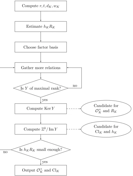
2.2 Definition of S-units performance, but at the risk of obtaining wrong results. On the other hand, one has to keep in mind that a too small factor basis makes the occurrence of elements which decompose over the factor basis more unlikely. We conclude that the right tuning of our factor basis size is crucial for the running time of the algorithm.

To sum up everything, our algorithm works essentially as follows (see also the flow chart shown in Figure 2.1). First we compute the constants r, t (see [Coh96, Algorithm 4.1.11]), the discriminant d

(see [Coh96, Algorithm 6.1.8]) as well as the number w

of roots of unity (see [Coh96, Algorithm 4.9.9]). Then we consult the analytic class number formula to get an estimation of the actual value of the product h

R

. We also choose an adequate factor basis p

, . . . , p

. Now we can start collecting relations until Y has a reasonable amount of columns. In particular, Y should have maximal rank, because we know that Cl

is finite. By computing Ker Y and Z

/ Im Y , we obtain candidates for O

and Cl

, respectively, and calculate the preliminary regulator and class number ˜ R

and ˜ h

. After that we need to check if ˜ h

R ˜

is already small enough. If not, we must go back and go on collecting more relations. In case ˜ h

R ˜

is close to our previously computed approximation, we succeeded and can transform the candidates for O

and Cl

in a canonical form to output them.

It is hard to predict the asymptotical running time of this algorithm, because the gen- eration of new relations is highly randomized. Although Buchmann’s algorithm for real quadratic fields is believed to be sub-exponential, Cohen does not claim this also holds for its generalization. In practice, however, this algorithm is very fast compared to other methods.

2.2 Definition of S-units

Before we introduce S-units, we first have to define S-integers.

Definition 2.1. Let S = {p

, . . . , p

} be a finite set of prime ideals in O

. The S- integers of K are defined as

O

:= {α ∈ K | v

(α) ≥ 0, p ∈ P

\ S} .

Clearly, O

= O

.

If we compare O

to O

, we simply discard the requirement that v

(α) ≥ 0 for all p ∈ S. Roughly spoken, O

arises from “inverting” the prime ideals p

, . . . , p

. Formally, O

is the localization of O

by an appropriate multiplicative set.

Proposition 2.2. Let (p

· · · p

)

= ωO

for some ω ∈ O

. Then O

is the

localization of O

by the multiplicative set {ω

| k ∈ N

}.

Proof. Since v

(ω) = 0 for all p ∈ P

\ S, it is clear that ω

O

⊂ O

for all k ∈ N

. On the other hand, for any α ∈ O

we can take k > max{−v

(α) | p ∈ S} to obtain v

(αω

) ≥ 0 for p ∈ S as well as for p ∈ P

\ S. Therefore, we conclude α ∈ ω

O

. Basic localization theory tells us that O

is a Dedekind domain again. Futhermore, there is a canonical bijection between prime ideals of O

which do not contain ω and the prime ideals of O

. The former ones are precisely P

\ S. Therefore, the group I

of O

-fractional ideals in K is basically the free abelian subgroup of I

generated by P

\ S.

Now we study the group of invertible elements in O

.

Definition 2.3. The units of the ring O

are called the S-units of K and are denoted by O

, i. e.

O

:= {α ∈ K | v

(α) = 0, p ∈ P

\ S} . As a consequence, every α ∈ O

admits a factorization

αO

= p

· · · p

.

Like before, O

differs from O

only by discarding the requirement v

(α) = 0 for all p ∈ S. If O

would be a principal ideal domain, say p

= p

O

for i ∈ {1, . . . , s}, we could simply write O

= p

× · · · × p

× O

. But in a general setting, the map O

→ Z

, α 7→ (v

(α))

is not surjective. Hence, the determination of O

is a little bit harder and depends on the class group, as we will see in the next section.

2.3 Computation of S-units

We can inductively obtain a set of generators for O

from a set of generators for O

s}

by adding a single generator, provided that we know the class group Cl

. The idea of studying the transition from S \ {p

} to S was taken from John Tate’s influential book [Tat84] about the Stark conjectures.

Proposition 2.4. There exists a γ ∈ K

with O

= γ

× O

s}

.

Proof. Denote by [p

] the class of p

in Cl

for all i ∈ {1, . . . , s}. Let m ∈ N be minimal with [p

]

∈ h[p

], . . . , [p

]i. Such an m exists because Cl

is finite. It follows that p

= γp

· · · p

for some γ ∈ K

and e

, . . . , e

∈ Z . Then

v

(γ) =











−e

if p ∈ {p

, . . . , p

} m if p = p

0 if p ∈ P

\ S .

2.4 The S-class group Therefore, we have γ ∈ O

and γ / ∈ O

s}

.

It remains to prove that every S-unit is a product of an (S \ {p

})-unit and a power of γ. Let α ∈ O

. Since v

(α) = 0 for all p ∈ / S, αO

= p

· · · p

with e

= v

(α) ∈ Z for i ∈ {1, . . . , s}. It follows that [p

]

· · · [p

]

is trivial in Cl

and thus [p

]

∈ h[p

], . . . , [p

]i. Because m was chosen minimal, we have e

= k · m for some k ∈ Z . We obtain α = γ

· αγ

with αγ

∈ O

s}

, since v

(αγ

) = e

− k · m = 0.

The proposition shows that a system of fundamental units for O

can be chosen to consist of a system of fundamental units for O

together with |S| additional free generators. In particular, Rank(O

) = |S| + Rank(O

) < ∞.

The proof of Proposition 2.4 already discloses a constructive method to compute these additional generators step by step. In practice, however, more efficient algorithms are used, which are able to compute a system of fundamental units for O

all at once.

One of them is described in [Coh00, Section 7.4.2]. Its further advantage is that the new generators are still in O

and have comparatively small coefficients.

Example 2.5. Let K = Q ( √

42) and S = {p} with p = (11, 3 + √

42). Obviously,

−1 is the only non-trivial root of unity contained in O

due to K ⊂ R . Thus, by the Dirichlet unit theorem O

= ε

× ε

with ε

= −1 and some fundamental unit ε

. It can be easily seen that ε

= 13 + 2 √

42 is a possible choice. Following the proof of Proposition 2.4, we need to find the order of p in Cl

. It turns out that p

is already principal, namely generated by ε

= 17 + 2 √

42, and we conclude O

= ε

× ε

×ε

.

2.4 The S -class group

The S-class group defined in this section is related to S-units and will be useful when we introduce and compute the (S, T )-class group.

Definition 2.6. The S-class group Cl

of K is defined as the class group of the Dedekind domain O

, i. e.

Cl

:= I

H

where I

is the group of fractional ideals in O

and H

is the subgroup of principal fractional ideals in O

.

The following proposition summarizes the roles of O

and Cl

in a compact way.

Proposition 2.7. The sequence

1

O

O

v

Z

λ

Cl

κ

Cl

1

is exact, where v(α) := (v

(α))

, λ(e

, . . . , e

) := [p

· · · p

] and κ is the homomor-

phism arising from a 7→ aO

by passage to the quotient.

Proof. By definition of O

and O

, it is obvious that O

= Ker v, so we have proven exactness at O

and O

.

Let (e

, . . . , e

) ∈ Im v, so there is an α ∈ O

with v

(α) = e

for i ∈ {1, . . . , s}.

Because v

(α) = 0 for p ∈ / S, we have αO

= p

· · · p

. Therefore, [p

· · · p

] is trivial in Cl

, which means (e

, . . . , e

) ∈ Ker λ. On the other hand, if (e

, . . . , e

) ∈ Ker λ, then [p

· · · p

] is trivial in Cl

. Hence, there exists an α ∈ K

such that αO

= p

· · · p

. But this implies α ∈ O

and v

(α) = e

for i ∈ {1, . . . , s}. It follows that (e

, . . . , e

) ∈ Im v.

Let [a] ∈ Im λ, so there exists (e

, . . . , e

) ∈ Z

such that [a] = [p

· · · p

]. Because pO

= O

for all p ∈ S, κ(a) = [p

]

· · · [p

]

is trivial in Cl

. Conversely, assume that [a] ∈ Ker κ. Then aO

= αO

for an α ∈ K

. Hence the prime decomposition of α

a contains only prime ideals from S. Therefore, [a] = [α

a] ∈ Im λ.

Finally, we prove the surjectivity of κ. Note that I

is generated by the prime ideals in O

. In Section 2.2, we mentioned the natural correspondence between P

\ S and the prime ideals in O

, which means that every prime ideal in O

is of the form pO

for some p ∈ P

\ S. It follows that the ideal classes κ([p]) where p ∈ P

\ S generate the whole class group Cl

.

As an immediate consequence of Proposition 2.7 we get Cl

∼ = Cl

/ h[p

], . . . , [p

]i .

In particular, Cl

is again finite and can be constructed easily from Cl

. Its cardinality

h

:= |Cl

| is called the S-class number.

3 From S -units to (S, T )-units

In this chapter, we will introduce (S, T )-units. We will present an algorithm for comput- ing them, which is the main goal of this thesis. After that we will enlarge on the related (S, T )-class group. By computing the (S, T )-class group we are able to verify the index of the (S, T )-unit group.

3.1 Idea and Definition

In 1996, Karl Rubin [Rub96] published an extension of the Stark conjectures where he studies Artin L-functions with higher order zeros at s = 0, arising from an additional set of prime ideals T. This set T results in a broad range of generalizations: From the S-unit group O

towards the (S, T )-unit group O

, from the S-class group Cl

towards the (S, T )-class group Cl

, from the S-zeta function ζ

towards the (S, T )- zeta function ζ

, from the S-class number formula towards the (S, T )-class number formula, and so on. In the following sections, we focus solely on O

and Cl

and discuss them independently of their relation to the Rubin Stark conjecture.

While the adoption of S-units “removes” certain prime ideals, thus enlarging O

to O

, the idea behind the additional set T is to “add” certain prime ideals (although they are already there), thus making O

smaller again into O

. In Section 3.4, we will see that an analogous picture happens to occur on the class groups Cl

, Cl

and Cl

.

Contrary to S-units, the (S, T )-units are not a unit group of a particular Dedekind domain. Instead they are defined directly as a subgroup of the S-units.

Definition 3.1. Let S and T be finite sets of prime ideals in O

with S ∩ T = ∅. The (S, T )-units of K are defined as

O

:= {α ∈ O

| α ≡ 1 (mod q), q ∈ T } . Clearly, O

= O

.

Let T be the product of the prime ideals in T. Using the Chinese remainder theorem, the above definition can be equivalently rewritten into a single condition:

O

= {α ∈ O

| α ≡ 1 (mod T)} .

However, the actual definition turns out to be quite as useful.

3.2 Computation of (S, T )-units

Let T = {q

, . . . , q

}. By definition, O

is the kernel of the map π : O

→

m

Y

i=1

(O

/q

)

where each α ∈ O

is sent to its projections in (O

/q)

for all q ∈ T . This is well-defined, because S ∩ T = ∅ implies that v

(α) = 0 for all q ∈ T .

In Section 2.3, we have seen that

O

= ε

× ε

× · · · × ε

for certain ε

, . . . , ε

∈ O

, where n = r + t + s. In other words, φ : Z /w

Z ⊕ Z

→ O

(x

, . . . , x

) 7→ ε

· · · ε

is an isomorphism between the additive group Z /w

Z ⊕ Z

and the multiplicative group O

.

Because O

/q

is always a finite field, (O

/q

)

is a cyclic group of order c

:= N (q

) −1 generated by some g

∈ (O

/q

)

. This implies that

ψ :

m

M

i=1

Z/c

Z →

m

Y

i=1

(O

/q

)

(a

, . . . , a

) 7→ (g

, . . . , g

)

is an isomorphism between the additive group

Z/c

Z and the multiplicative group

i=1

(O

/q

)

.

Therefore, the problem of computing O

reduces to computing the kernel of the homomorphism

A : Z /w

Z ⊕ Z

→

m

M

i=1

Z /c

Z

defined as A := ψ

◦ π ◦ φ, as shown in the following commutative diagram with exact rows:

1

O

O

π

i=1

(O

/q

)

0

Ker A

φ|

∼ =

OO

Z /w

Z ⊕ Z

A

φ ∼ =

OO

m

M

i=1

Z /c

Z ψ ∼ =

OO

3.2 Computation of (S, T )-units In particular, we get (O

: O

) = | Im A| ≤

c

< ∞ and thus Rank O

= Rank O

.

More explicitly, one has to solve the system of linear congruences a

x

+ · · · + a

x

≡ 0 (mod c

) , i = 1, . . . , m

in integers x

, . . . , x

(to be more precisely, we have x

∈ Z/w

Z ), where the coefficient a

is given by the i-th component of ψ

(π(ε

)), which is the discrete logarithm of ε

in (O

/q

)

. This system of linear congruences is equivalent to the system of linear equations

a

x

+ · · · + a

x

+ c

y

= 0 , i = 1, . . . , m

over Z in n + m variables x

, . . . , x

, y

, . . . , y

. Hence, it remains to find a Z -basis for the kernel space of the matrix

M :=













a

a

· · · a

c

0 · · · 0 a

a

· · · a

0 c

· · · 0 .. . .. . . .. .. . .. . .. . . .. .. . a

a

· · · a

0 0 · · · c













∈ Z

,

for which efficient algorithms are known.

Therefore, we have developed the following algorithm for the (S, T )-unit group.

Algorithm 3.2 (Computation of (S, T )-units). Let T = {q

, . . . , q

}.

1. [Compute S-units.] Use the algorithm from Section 2.3 to compute fundamental units ε

, . . . , ε

of O

.

2. [Take discrete logarithms.] For i = 1, . . . , m and j = 1, . . . , n set a

to be the discrete logarithm of ε

in the residue class field O

/q

.

3. [Solve linear equations.] Construct a Z -basis of the kernel space of the matrix M defined as above where c

:= N (q

) − 1.

4. [Terminate.] For every kernel vector (x

, . . . , x

, y

, . . . , y

) from step 3, output the fundamental unit φ(x

, . . . , x

) = ε

· · · ε

of O

.

The running time of this algorithm is dominated by the first step where the S-units are computed. Therefore, the computational complexity of finding fundamental (S, T )-units is not bigger than the one of finding fundamental S-units, which in turn is substantially ruled by the unit group computation.

We demonstrate the operation of Algorithm 3.2 on a small example.

Example 3.3. Let K = Q ( √

42), S = {p}, T = {q

, q

} with p = (11, 3 + √

42) (one of the two prime ideals lying above 11 in O

), q

= (5) (the unique principal prime ideal lying above 5 in O

) and q

= (7, √

42) (the unique prime ideal lying above 7 in O

).

1. [Compute S-units.] Example 2.5 resulted in O

= ε

× ε

× ε

with ε

= −1, ε

= 13 + 2 √

42 and ε

= 17 + 2 √ 42.

2. [Take discrete logarithms.] The residue class fields are O

/q

∼ = F

∼ = F

( √ 2) and O

/q

∼ = F

. We choose the generators g

= 3 + √

2 of F

( √

2) and g

= 3 of F

and calculate

O

→

F

( √

2) × F

→ Z /24 Z ⊕ Z /6 Z ε

7→ (4, 6) 7→ (12, 3)

ε

7→ (3 + 2 √

2, 6) 7→ (4, 3) ε

7→ (2 + 2 √

2, 3) 7→ (8, 1) .

3. [Solve linear equations.] To solve the system of linear congruences 12x

+ 4x

+ 8x

≡ 0 (mod 24)

3x

+ 3x

+ x

≡ 0 (mod 6) , we determine the kernel of the matrix

M = 12 4 8 24 0

3 3 1 0 6

!

∈ Z

to be

*















2 0 0

−1

−1















,















−1 3 0 0

−1















,















0 0 6

−2

−1













 +

.

4. [Terminate.] Applying φ yields ε

= 1, ε

ε

= −8749 − 1350 √

42 and ε

= 361703161 + 55811340 √

42. We can see that the Z /2 Z -torsion was eliminated and O

contains no non-trivial roots of unity. This yields the two fundamental units −ε

and ε

.

Many additional examples can be found in Chapter 4.

3.3 Implementation within Magma

The computational algebra system Magma was chosen to implement Algorithm 3.2. It

already provides the routine SUnitGroup to compute the group of S-units. Because

abelian groups are represented in Magma as quotients of Z

, SUnitGroup additionally

returns the isomorphism φ defined in the previous section viewed as an injection into K,

3.3 Implementation within Magma i. e. the system of fundamental units for O

is given by the images under φ of the n canonical generators of Z /w

Z ⊕ Z

.

For convenience, the newly implemented routine STUnitGroup returns apart from the (S, T )-unit group also the S-unit group together with its map into the field. Because the computed (S, T )-unit group is represented in Magma as a subgroup of the S-unit group, this map into K can be applied to elements of the (S, T )-unit group as well.

1

intrinsic STUnitGroup(S :: [ RngOrdIdl ], T :: [ RngOrdIdl ]) −> GrpAb, GrpAb, Map

2

{Compute (S,T)−units.}

3

require not (IsEmpty(S) and IsEmpty(T)):

4

"At least S or T must be non-empty.";

5

require IsDisjoint (SequenceToSet(S), SequenceToSet(T)):

6

"S and T must be disjoint.";

7

if IsEmpty(S) then

8

O := Order(T[1]);

9

U, mU := UnitGroup(O);

10

else

11

U, mU := SUnitGroup(S);

12

end if ;

13

m := #T;

14

n := NumberOfGenerators(U);

15

M := ZeroMatrix(IntegerRing(), m, n + m);

16

for i := 1 to m do

17

F, mF := ResidueClassField(T[i ]);

18

for j := 1 to n do

19

x := mU(U.j);

20

r := mF(x);

21

M[i, j ] := Log(r);

22

end for;

23

M[i, n + i] := #F − 1;

24

end for;

25

K := KernelMatrix(Transpose(M));

26

L := RowSequence(ColumnSubmatrix(K, n));

27

V := sub<U | L>;

28

return V, U, mU;

29

end intrinsic ;

Example 3.4. We demonstrate how to do Example 3.3 in Magma. First we need to attach the file where STUnitGroup is implemented.

> Attach("STUnitGroup.m");

Then we create K = Q ( √

42) and O

, as well as the three prime ideals p, q

and q

.

> K := QuadraticField(42);

> O := MaximalOrder(K);

> p := Decomposition(O, 11)[1][1];

> q1 := Decomposition(O, 5)[1][1];

> q2 := Decomposition(O, 7)[1][1];

> p;

Prime Ideal of O

Two element generators:

11

$.2 + 3

Now we are ready to call STUnitGroup and view the results.

> V, U, mU := STUnitGroup([p], [q1, q2]);

> U;

Abelian Group isomorphic to Z/2 + Z + Z Defined on 3 generators

Relations:

2*U.1 = 0

> V;

Abelian Group isomorphic to Z + Z

Defined on 2 generators in supergroup U:

V.1 = 3*U.2

V.2 = 6*U.3 (free)

We can use the returned map to explicitly obtain the fundamental (S, T )-units.

> mU(V.1), mU(V.2);

-8749/1*O.1 - 1350/1*O.2

361703161/1*O.1 + 55811340/1*O.2

Finally, we are interested in the index (O

: O

).

> Index(U, V);

36

3.4 The (S, T )-class group

The (S, T )-class group can be understood as kind of a ray class, as the following definition

suggests.