Elastic Wave Propagation in Granular Packings
Inaugural-Dissertation
zur
Erlangung des Doktorgrades
der Mathematisch-Naturwissenschaftlichen Fakultät der Universität zu Köln
vorgelegt von Karsten Tell aus Lauf a. d. Pegnitz
Köln, 2020
(Gutachter)
Tag der mündlichen Prüfung:
Prof. Dr. Stefan Luding Prof. Dr. Xiaoping Jia
14. August 2020
Ich widme diese Arbeit meinen Eltern Alfred und Olympia Tell.
Abstract
Jammed packings of granular materials such as sand, powders or glass beads show an effective elastic behavior. For a given confinement pressurep0, volume fractionφ and coordination numberZan effective bulk- and shear-modulus arises which can be probed by measurements of the speed of sound for longitudinal and transverse elastic waves. For sufficiently high confinement pressure, low dynamic pressure and long wavelengths, wave propagation is well approximated by effective medium theory.
At increasing amplitude or decreasing static pressure the effect of nonlinearities becomes increasingly noticeable. This results from nonlinear, dissipative and hysteretic contact forces on the microscopic scale and rearrangements in the force-chain network on the mesoscopic scale.
At low amplitudes, weakly-nonlinear behavior is found as a small correction to the linear elastic- ity. This leads to demodulation of incident waves, frequency-mixing and mode conversion between longitudinal and transversal waves. Upon vibrations of higher amplitudes, the static friction and static precompression are overcome, leading to irreversible changes in the force-chain network and elastic weakening. The wavefront speed drops in this intermediate amplitude regime. In the high-amplitude regime, when the dynamic pressure exceeds the static pressure, shock-like behavior with a characteris- tic increase in wavefront speed arises.
In this thesis, a fully automated experimental apparatus for elastic wave measurements at low con- finement pressure was developed and used on a DLR sounding rocket campaign. During the micro- gravity phase of the MAPHEUS8 mission, packings in the pressure range of 20 to 400 Pa were prepared and sound transmission at amplitudes varying by two orders of magnitude was measured. At the lowest amplitudes a linear regime with sound speed from 60 to 160ms is found. The pressure dependence of the sound speed is found to vary withpν0,νbeing close to 1/3, deviating from the 1/6 exponent valid for high pressure and from the 1/4 exponent, previously reported in the literature to describe the low pressure behavior. Comparison with literature data at higher pressures suggests a continous increase of the exponent with pressure, similar to findings for 2D systems reported in the literature. In the present analysis, the logarithmic derivative is found constant over at least five orders of magnitude of pressure.
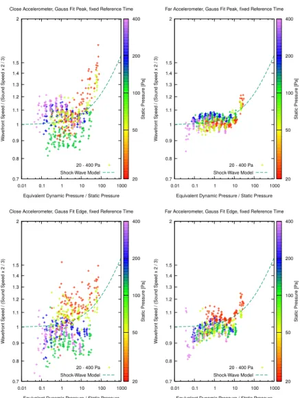
Furthermore, for the highest amplitudes a drop in the wavefront-speed with increasing amplitude is found forp0between 100 and 400 Pa, suggesting elastic weakening, while for 20 and 50 Pa a rising wavefront speed is observed, suggesting shock-like behavior. Wave-front attenuation is found to be increased at the highest amplitudes, in agreement with previous results for shock-waves in glass bead packings on ground.
To further investigate wave propagation beyond effective medium theory, and to probe possible long correlation lengths related to anisotropy and unjamming, measurements of multiply-scattered elastic waves were conducted on ground withp0∝1 kPa. In measurements of the configurationally averaged incoherent intensity in the diffusive regime, the transport mean-free path is found between 1.6 and 1.8 bead diameters for a sample of small height, moderately affected by a hydrostatic gradient and close to 5 bead diameters for a larger sample affected by a much larger gradient. Similar values are found for the scattering mean-free path extracted from the attenuation of the coherent signal with varying sample thickness. These results are larger than literature values obtained at much higher pressure, where the hydrostatic gradient becomes negligible.
Finally, inverse-filtering and time-reversal techniques in a two transducer setup were used to measure wave focussing, to test it as a method for measuring microscopic rearrangements in the granular packing due to external excitation.
Kurzzusammenfassung
Verhakte (engl. ’jammed’) Granulatpackungen aus Materialien wie Sand, Pulvern oder Glaskugeln zeigen ein effektives elastisches Verhalten. Bei gegebenem Einschlussdruckp0, Volumenanteilφund KoordinationszahlZzeigt sich ein effektiver Kompressions- und Schermodul, welcher durch Messung der Schallgeschwindigkeit longitudinaler und transversaler elastischer Wellen untersucht werden kann.
Bei hinreichend hohem Einschlussdruck, niedrigem dynamischem Druck und großer Wellenlänge ist die Wellenausbreitung in guter Näherung durch die Theorie des effektiven Mediums beschrieben.
Bei steigender Amplitude oder sinkendem statischem Druck wird der Effekt von Nichtlinearitäten zunehmend stärker bemerkbar. Auf der mikroskopischen Skala resultiert dies aus nichtlinearen, dis- sipativen und hysteretischen Kontaktkräften und auf der mesoskopischen Skala aus Umlagerungen im Netzwerk der Kraftketten.
Bei niedrigen Amplituden wird schwach-nichtlineares Verhalten im Sinne einer kleinen Korrek- tur zur linearen Elastizität beobachtet. Dies führt zu Demodulation einfallender Wellen, Frequenz- Mischung und Modenkonversion zwischen longitudinalen und transversalen Wellen. Vibrationen höher- er Amplitude überwinden statische Reibung wie auch Vorspannung der Kontakte, sodass irreversible Änderungen im Netzwerk der Kraftketten sowie elastischer Festigkeitsabfall auftreten. In diesem mit- tleren Amplitudenbereich fällt die Geschwindkeit der Wellenfront ab. Bei hohen Amplituden, wenn der dynamische Druck den Statischen übersteigt, zeigt sich Schockwellen-artiges Verhalten mit charakter- istischem Anstieg der Geschwindigkeit der Wellenfront.
In dieser Arbeit wurde ein vollautomatischer experimenteller Apparat für Messungen elastisch- er Wellen bei niedrigem Einschlussdruck entwickelt und im Rahmen einer Messkampagne auf ein- er Höhenforschungs-rakete des DLR eingesetzt. Im Laufe der Mikrogravitationsphase während der MAPHEUS 8 Mission wurden Packungen mit Drücken zwischen 20 und 400 Pa präpariert und die Schalltransmission in einem Amplitudenbereich über zwei Größenordnungen gemessen. Bei den niedrig- sten Amplituden zeigte sich ein linearer Bereich mit Schallgeschwingkeiten zwischen 60 und 160 m/s.
Die Druckabhängigkeit schwankte wiepν0 mitνnahe an 1/3, im Kontrast zum Exponenten 1/6, der bei hohen Drücken gilt, und zu 1/4, dem bisherigen Literaturwert zur Beschreibung des Niedrigdruck- verhaltens. Der Vergleich mit Messwerten aus der Literatur bei höheren Drücken suggeriert einen kon- tinuierlichen Anstieg des Exponenten mit dem Druck, vergleichbar mit dem Befund zum Verhalten zweidimensionaler Systeme in der Literatur. In der vorliegenden Auswertung zeigt sich, dass die loga- rithmische Ableitung des Exponenten über mindestens 5 Größenordnungen des Drucks konstant ist.
Bei den höchsten Amplituden zeigt sich ein Abfall der Geschwindigkeit der Wellenfront mit steigen- der Amplitude fürp0zwischen 100 und 400 Pa, ein Anzeichen für elastichen Festigkeitsabfall, während zwischen 20 und 50 Pa eine steigende Geschwindigkeit der Wellenfront sichtbar wird, ein Anzeichen für Schockwellen-artiges Verhalten. Die Dämpfung der Wellenfront ist bei den höchsten Amplituden erhöht - in Übereinstimmung mit bekannten Resultaten für Schockwellen in Glaskugelpackungen am Boden.
Zur weiteren Untersuchung der Wellenausbreitung jenseits der Theorie des effektiven Mediums und zur Untersuchung möglicher großer Korrelationslängen die in Zusammenhang mit Anisotropie und Verlust der mechanischen Rigidität (engl. ’unjamming’) stehen, wurden Versuche zur Mehrfach- streuung elastischer Wellen bei Bodenmessungen mit p0∝1 kPa durchgeführt. In Messungen der Konfigurations-gemittelten inkohärenten Intensität im diffusen Bereich zeigte sich eine mittlere freie Weglänge des Transports zwischen 1,6 und 1,8 Kugeldurchmessern im Falle kleiner Probenhöhe mit einem moderaten hydrostatischen Gradienten sowie ungefähr 5 Kugeldurchmessern im Falle einer größeren Probe mit deutlich größerem Gradienten. Vergleichbare Werte nimmt die mittlere freie Weglänge
der Streuung an, die aus der Dämpfung des koheränten Signals bei verschiedener Probendicke bes- timmt wurde. Diese Resultate sind größer als Literaturwerte, gemessen bei wesentlich höherem Druck, bei welchem der hydrostatische Gradient vernachlässigbar ist.
Schließlich wurden Dekonvolutions- und Zeitumkehr-Techniken in einem Aufbau aus zwei Wan- dlern verwendet um Wellenfokussierung zu messen, um diese als Methode zur Messung mikroskopis- cher Umordnungen in der Granulatpackung unter externer Anregung zu testen.
Acknowledgements / Danksagung
Here I would like to thank the various people who helped making my PhD thesis possible:
I thank my supervisor Prof. Matthias Sperl and leader of the granular group at DLR for giving me the opportunity to pursue this work and conduct related experiments in the various microgravity envi- ronments.
Thanks to Christoph Dreißigacker, the engineer at DLR who not only made GRASCHAflight-worthy but managed the difficult but highly successful sounding rocket campaign in Kiruna with many exper- iments from our institute.
Special thanks to the engineering students who contributed to the development of granular sound in- struments at our institute, especially Alberto Chiengue Tchapnda without whom no GRASCHArocket module would exist, also Alex Kamphuis and Antoine Micallef, who worked on previous campaigns involving parabolic flight experiments.
A big thank you to Dr. Peidong Yu for proof-reading as well as many in-depth discussions about my work and the experience and knowledge he shared with me based on his previous work on granular sound, a field of research which he introduced at DLR many years ago.
Thanks to the team at the DLR workshop who flawlessly manufactures the required parts for exper- iments.
Thanks to Dr. Till Kranz for proof-reading and many scientific discussions.
Thanks to Dr. Juan Petit, Dr. Olivier Coquand, Dr. Koray Önder, Dr. Philip Born, Dr. Jan Haeberle, Dr. Nishant Kumar and Dr. Sebastian Pitikaris for interesting scientific discussions. Further thanks to the other current and former members of the granular group, such as Dr. Masato Adachi, Dr. Ali Kaouk, Dr. Miranda Fateri, Dr. Alexandre Meurisse, Olfa Lopez, Merve Seckin-Krüger and many others for further interesting discussions. You made the time at DLR worthwhile and never boring.
This also involved many unbelievable kicker games which shall be remembered.
Ich möchte meinen Eltern Alfred und Olympia dafür danken, dass sie mir die Voraussetzungen für ein gutes Leben geschaffen haben und mir von klein auf eine Begeisterung für Wissenschaft und Bildung vermittelt haben. Ihnen, speziell meinem Vater, der das Ergebnis dieser Arbeit leider nicht mehr zu sehen bekommen kann, sei diese Arbeit gewidmet.
Contents
Abstract ii
Kurzzusammenfassung iii
Acknowledgements . . . v
1. List of Figures . . . ix
List of Abbreviations x List of Symbols xii Introduction 1 1. Theory of Elastic Waves in Granular Matter 4 1.1. Introduction . . . 4
1.2. The Linear Chain . . . 4
1.2.1. Homogeneous, Free Chain in the Continuum Limit . . . 4
1.2.2. Homogeneous, Driven Chain in the Continuum Limit . . . 7
1.2.3. High-Frequency Behavior in the Monodisperse Chain . . . 9
1.2.4. Bidisperse Chain: Bandgaps and Optical Modes . . . 11
1.2.5. The Hertzian Chain: Linear Waves . . . 13
1.2.6. Solitons in the Hertzian Chain . . . 15
1.2.7. Weak Disorder and Linear Waves . . . 17
1.3. The Dense Packing . . . 22
1.3.1. Linear Elasticity in 3D . . . 22
1.3.2. Effective Medium Theory . . . 28
1.3.3. Jiang-Liu Elasticity . . . 29
1.3.4. Disorder and Multiple Scattering . . . 30
2. Acoustic Wave Measurements at Low Connement Pressure 35 2.1. Introduction . . . 35
2.2. Preliminary Developments . . . 36
2.3. The Grascha 2 Apparatus . . . 37
2.3.1. Requirements . . . 37
2.3.2. Setup Overview . . . 39
2.3.3. Packing Preparation . . . 44
2.3.4. Acoustic Excitation . . . 48
2.3.5. Inverse Filtering . . . 48
2.3.6. Measurement Sequence in Microgravity . . . 52
2.4. Results . . . 53
2.4.1. Force Distribution on Ground . . . 53
2.4.2. Wavefront Speed on Ground . . . 53
2.4.3. Force Distribution in Microgravity . . . 56
2.4.4. Wavefront Speed in Microgravity . . . 56
2.4.5. Attenuation of Wavefront . . . 59
2.5. Discussion . . . 66
2.5.1. Linear Regime . . . 66
2.5.2. Nonlinear Regime . . . 68
2.5.3. Attenuation . . . 69
2.6. Conclusion and Outlook . . . 70
3. Measurement of Multiple Scattering 73 3.1. Introduction . . . 73
3.2. Setup Overview . . . 75
3.2.1. GRASCHASetup . . . 75
3.2.2. 3D-printed Sample Cell . . . 75
3.3. Incoherent Intensity Profile . . . 77
3.3.1. Measurement Procedure with GRASCHA . . . 79
3.3.2. Measurement Procedure with 3D-printed Cell . . . 80
3.3.3. Results from GRASCHA . . . 81
3.3.4. Results from 3D-printed Cell . . . 82
3.3.5. Discussion . . . 83
3.4. Coherent Attenuation . . . 83
3.4.1. Procedure . . . 84
3.4.2. Result from 3D-printed Cell . . . 84
3.4.3. Discussion . . . 85
3.5. Wave Focussing and Time Reversal . . . 85
3.5.1. Introduction . . . 85
3.5.2. Setup Overview . . . 86
3.5.3. Focussing in Air and in Granular Matter . . . 86
3.5.4. Evolution under Tapping . . . 88
3.5.5. Time Reversal . . . 89
3.5.6. Discussion . . . 90
3.6. Conclusion and Outlook . . . 91
4. Conclusion and Outlook 96 Appendices A. Additional Grascha 2 Data 99 A.1. Results from Sound Measurements . . . 100
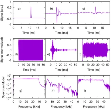
A.2. Raw Signals . . . 105
B. Overview of Grascha 2 Experiment Software 111 B.1. Overview . . . 112
B.2. Low-Level Programs . . . 113
B.2.1. Picoscope and Picolog programs . . . 113
B.2.2. Arduino Code . . . 114
B.2.3. Arduino Serial Communication Program . . . 114
B.3. High-Level Programs . . . 115
B.3.1. Sound-Control . . . 115
B.3.2. Measurement-Monkey . . . 116
B.4. User Interface . . . 117
B.4.1. Hypersound HTTP-Server and Web-interface . . . 117
B.4.2. Command Line Interfaces . . . 118
C. Overview of quick (Grascha 2 Analysis Tool) 120
D. Analysis Methods 124
D.1. FFT . . . 125
D.2. Time-Frequency-Analysis . . . 126
D.3. Causal Time-Frequency-Analysis . . . 129
D.4. Sensor Response . . . 130
E. Further Calculations 133 E.1. Displacement Field Theory . . . 134
E.2. Calculation of Scattering Mean Free Path . . . 134
E.2.1. Operator Potential and Correlation Functions . . . 134
E.2.2. Calculation based on Helmholtz Equation . . . 135
E.2.3. Calculation based on Schrödinger Equation . . . 138
1. List of Figures
1.1. Contours for Complex Integral . . . 8
1.2. Dispersion Relation in Monodisperse Chain . . . 10
1.3. Dispersion Relation in Bidisperse Chain . . . 12
1.4. Nonlinear Frequency-Mixing . . . 16
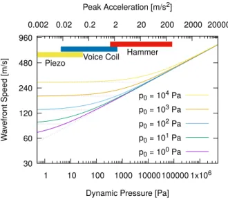
2.1. Acoustic Excitation Parameter Range . . . 39
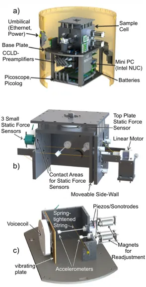
2.2. Grascha 2Experimental Setup Overview . . . 41
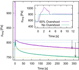
2.3. Drop Tower Test of Pressure Control Loop . . . 45
2.4. Packing Preparation Protocol for Grascha 2 . . . 46
2.5. Inverse Filtering of Excitation Signal . . . 51
2.6. Wavefront Speed on Ground . . . 54
2.7. Test Measurement of Wavefront Speed in Vacuum-Chamber . . . 55
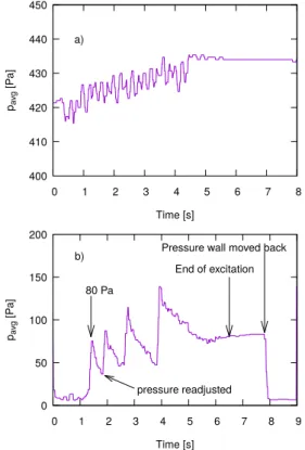
2.8. Static Pressure in Microgravity . . . 57
2.9. Force Anisotropy in Microgravity . . . 57
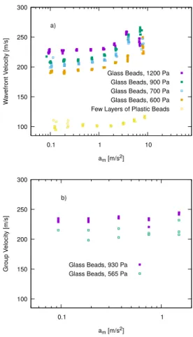
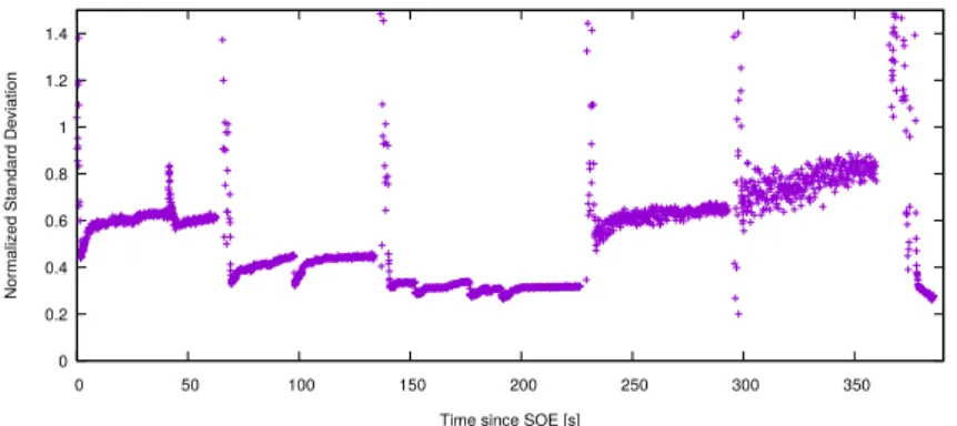
2.10. Standard Deviation of Static Force at different Positions at Side-Wall in Microgravity . 60 2.11. Wavefront Speed from 2 Accelerometer Signals . . . 61
2.12. Wavefront Speed from Single Sensor Signal Peak . . . 62
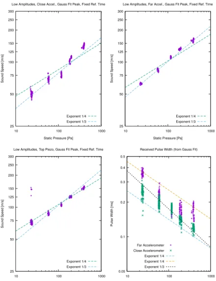
2.13. Pressure Dependence of Sound Speed and Pulse Width . . . 63
2.14. Master Plots of Wavefront Speed . . . 64
2.15. Wavefront Attenuation in Microgravity . . . 65
2.16. Sound Speed Power-Law Exponent vs. Logarithm of Pressure . . . 67
2.17. Sound Speed Fit Model . . . 68
3.1. 3D-printed Sound Cell Overview . . . 76
3.2. Bender Element for Measurement/Excitation of Transversal Waves . . . 76
3.3. Devices of the Measurement Chain for Multiple Scattering Measurements . . . 77
3.4. Tone-burst Transmission in GRASCHA . . . 82
3.5. Incoherent Intensity in GRASCHA . . . 82
3.7. Intensity Profile and Diffusion Fit for Varying Sample Thickness . . . 83
3.8. Coherent Attenuation in 3D-printed Cell . . . 85
3.9. Accelerometers for Focussing Measurements . . . 86
3.10. Probe Signal for Focussing . . . 87
3.11. Focussing in Air and Granular Matter . . . 88
3.12. Evolution of Focussed Signal during Tapping . . . 89
3.13. Time Reversal Measurement . . . 90
3.6. Incoherent Intensity in 3D-printed Cell . . . 92
A.1. Resemblance, Wavefront Speed and Pressure vs Time . . . 100
A.2. Coherence of 2 - 11 kHz Tone-bursts in Microgravity . . . 102
A.3. Peak Velocity vs. Peak Acceleration at Wavefront . . . 103
A.4. Wavefront Speed from Single Sensor Signal Threshold . . . 104
A.5. Acceleration Signals at Largest Amplitude . . . 105
A.6. Acceleration Signals at Small Amplitude . . . 106
A.7. Velocity Signals at Largest Amplitude . . . 107
A.8. Velocity Signals at Small Amplitude . . . 108
A.9. Displacement Signals at Largest Amplitude . . . 109
A.10.Displacement Signals at Small Amplitude . . . 110
B.1. Overview ofGrascha 2Software . . . 112
B.2. Grascha 2 Web-interface . . . 119
D.1. Group Delay from measured Signal Envelope . . . 128
D.2. Smoothed Pseudo-Wigner-Ville Distribution of measured Response . . . 129
List of Abbreviations
DLR Deutsches Zentrum für Luft- und Raumfahrt (German Aerospace Center) EMT Effective Medium Theory
GRASCHA Granular Sound Characterization experiment / Granulat Schall Experiment MAPHEUS Materialphysikalische Experimente unter Schwerelosigkeit
(material physics experiments at zero gravity)
ZARM Zentrum für angewandte Raumfahrttechnologie und Mikrogravitation Center of Applied Space Technology and Microgravity
AWG Arbitraty Waveform Generator FFT Fast Fourier Transform
NUC Next Unit of Computing (mini-pc by Intel, used inGrascha)
SOE Start of Experiment (signal that indicates the start of the microgravity period) SODS (signal that enables the on-board power-supply)
SCP Secure Copy Protocol
SSH Secure Shell
List of Symbols
i √
−1, unless used as an index, which will be obvious
cpandcs longitudinal / P-wave sound speed and transverse / S-wave sound speed p0andpi static / confinement pressure and dynamic pressure
am geometric mean of peak acceleration of two sensors
Z mean contact/coordination number
φ volume ratio
λandµ (effective) Lamé moduli, unlessλis used for the wavelength
ρ (bulk material) density
u(x,t) displacement
εij(x,t) infinitesimal strain tensor σij(x,t) Cauchy stress tensor
ijk Levi-Civita symbol
Ψ(x,t) (vector-valued) wave function derived fromu(x,t)andεi j(x,t)
H(x)andδH(x) time-evolution operator and random inhomogeneity / perturbation operator
`c correlation length
`s scattering mean free path
`T transport mean free path τa inelastic absorption time
Q quality factor
ω angular frequency, or center frequency
Ω modulation angular frequency
k0 =ω/c, wave-number in long-wavelength limit of homogeneous wave-equation
Σ(ω) self-energy at angular frequencyω
(if no dependence on ork : then it is used to indicate a sum)
Introduction
Systems of discrete particles of sufficient mass and size, such that no Brownian motion is observed, which are interacting with dissipative forces, such that they come to rest unless externally driven, are referred to as ’granular’[1, 2].
Granular matter is known for having unusual properties that are a currently active field of research.
For example, granular gasses show unconventional damping behavior[3] and negative heat capacity[4].
But even when granular material is brought to rest and confined to a volume under pressure, nontriv- ial behavior can still be found: elastic waves, which propagate through an effective medium[5, 6, 7]
provided by the elastic response of the packing in the long wavelength limit, propagate linearly until they are scattered and attenuated by disorder[8], affected slowed down or broadened by dispersion[9]
or distorted by demodulation and frequency-mixing at nonlinear contacts[10]. At vanishing confine- ment pressure, solitons[11, 12] and shock-waves [13, 14] are found. For high frequencies, where the wavelength is comparable to the particle diameter, multiple scattering and diffusive transport is found[15, 16]. At lower frequencies, when the density of state is examined, a cross-over from Debye- like increase to a plateau is found at a characteristic frequency that increases with pressure[17, 18] and implies a diverging length scale at the jamming point.
In this thesis, elastic wave propagation in granular matter beyond effective medium theory is exam- ined by experiments in glass bead packings at low confinement pressure.
In chapter 1 an overview of wave phenomena in granular matter is given, introducing linear waves, dispersion, parametric mixing and demodulation, solitons and scattering, first in the granular chain, later addressing the three-dimensional packing.
In chapter 2 the GRAnular Sound CHAracterization or GRASCHAexperiment is presented, as re- cently published[19]. Measurement results from a sounding rocket campaign in 2019 are shown, which probe linear and nonlinear elastic waves in glass bead packings at low confinement pressure. A univer- sal pressure dependence of the sound speed is suggested.
In chapter 3 measurements of multiply scattered elastic waves are shown. First, the incoherent intensity in ensembles of macroscopically equivalently prepared packings is investigated. Then, the coherent attenuation is measured. Finally, wave focussing techniques are tested.
In chapter 4 an overall conclusion is given.
Bibliography
[1] Heinrich M Jaeger and Sidney R Nagel. Physics of the granular state.Science, 255(5051):1523–
1531, 1992.
[2] Heinrich M Jaeger, Sidney R Nagel, and Robert P Behringer. Granular solids, liquids, and gases.
Reviews of modern physics, 68(4):1259, 1996.
[3] Marcus N Bannerman, Jonathan E Kollmer, Achim Sack, Michael Heckel, Patric Mueller, and Thorsten Pöschel. Movers and shakers: Granular damping in microgravity. Physical Review E, 84(1):011301, 2011.
[4] Nikolai V Brilliantov, Arno Formella, and Thorsten Pöschel. Increasing temperature of cooling granular gases.Nature communications, 9(1):1–9, 2018.
[5] Jacques Duffy and R.D. Mindlin. Stress-strain relation and vibrations of a granular medium. J.
Appl. Mech., ASME, 24:585–593, 1957.
[6] P. J. Digby. The effective elastic moduli of porous granular rocks. J. Appl. Mech., 48(4):803, 1981.
[7] K. Walton. The effective elastic moduli of a random packing of spheres. J. Mech. Phys. Solids, 35(2):213 – 226, 1987.
[8] O Mouraille and Stefan Luding. Sound wave propagation in weakly polydisperse granular mate- rials.Ultrasonics, 48(6-7):498–505, 2008.
[9] Christophe Coste and Bruno Gilles. Sound propagation in a constrained lattice of beads: High- frequency behavior and dispersion relation.Phys. Rev. E, 77:021302, Feb 2008.
[10] V Tournat, VE Gusev, and B Castagnede. Self-demodulation of elastic waves in a one- dimensional granular chain.Physical Review E, 70(5):056603, 2004.
[11] VF Nesterenko. Propagation of nonlinear compression pulses in granular media.J. Appl. Mech.
Tech. Phys. (Engl. Transl.), 24(5):733–743, 1983. Translated from Zhurnal Prikladnoi Mekhaniki i Tekhnicheskoi Fiziki, No. 5, pp. 136-148, September-October, 1983.
[12] C. Daraio, V. F. Nesterenko, E. B. Herbold, and S. Jin. Strongly nonlinear waves in a chain of teflon beads.Phys. Rev. E, 72:016603, Jul 2005.
[13] Leopoldo R. Gómez, Ari M. Turner, Martin van Hecke, and Vincenzo Vitelli. Shocks near jam- ming.Phys. Rev. Lett., 108:058001, Jan 2012.
[14] Siet van den Wildenberg, Rogier van Loo, and Martin van Hecke. Shock waves in weakly com- pressed granular media.Phys. Rev. Lett., 111:218003, Nov 2013.
[15] X. Jia. Codalike multiple scattering of elastic waves in dense granular media. Phys. Rev. Lett., 93:154303, Oct 2004.
[16] XiaoPing Jia, J Laurent, Yacine Khidas, and Vincent Langlois. Sound scattering in dense granular media.Chinese Science Bulletin, 54(23):4327–4336, 2009.
[17] Leonardo E Silbert, Andrea J Liu, and Sidney R Nagel. Vibrations and diverging length scales near the unjamming transition.Physical review letters, 95(9):098301, 2005.
[18] Eli T Owens and Karen E Daniels. Acoustic measurement of a granular density of modes.Soft Matter, 9(4):1214–1219, 2013.
[19] Karsten Tell, Christoph Dreißigacker, Alberto Chiengue Tchapnda, Peidong Yu, and Matthias Sperl. Acoustic waves in granular packings at low confinement pressure. Review of Scientific Instruments, 91(3):033906, 2020.
1. Theory of Elastic Waves in Granular Matter
1.1. Introduction
As a stating point for this thesis, a brief theoretical introduction is given to show the various elastic wave phenomena encounterd in granular media. Some instructive calculations and references to the relevant literature are provided. In section 1.2 linear wave propagation, dispersion, weakly-nonlinear effects and solitons are introduced as well as multiple scattering. This is done in a one-dimensional system, the granular chain, which is convenient for calculations and already shows many aspects of the behaviour of granular packings qualitatively. In section 1.3 the three-dimensional case is intruduced, which is more relevant for the experiments in this thesis.
1.2. The Linear Chain
1.2.1. Homogeneous, Free Chain in the Continuum Limit
To demonstrate how wave-like behavior can arise in a granular medium, let us first consider a linear chain of N particles within total length L. Each particle of index i at positionxi has a massmiand is interacting with its neighbor at i+1 through a linear spring of stiffnesski and similarly with its neighbor at i-1 through a spring of stiffnesski−1. The behavior at i=0 and i=N depends on the boundary conditions, which can represent open chains with fixed positions (Dirichlet) or velocities (Neumann) of the particles at the ends or closed chains (periodic boundary conditions). To simplify the calculations in this introductory example we choose the latter and will address the other cases in later chapters when appropriate. Hence, here we letki−N=kias well asmi−N=miandxi−N=xi. In the simplest caseki=const.=kandmi=const.=m. Then in the ground state all particles are evenly spaced at xi=i·L/Nand Newton’s equations of motion[1] are given by:
mid2
dt2xi=k·((xi+1−xi−L/N)−(xi−xi−1−L/N)) (1.1) We can express (1.1) in terms of the particle displacementui=xi−i·L/N:
mid2
dt2ui=k·(ui+1+ui−1−2·ui) (1.2) Even though the system is discrete, we can always describe the displacement by a continuous func- tionu(x,t)that fulfillsu(xi,t) =ui(t). Let us assumeuvaries on a characteristic length scaleλ. Then it is convenient to writeu(x,t) =u(xi+λ·ξ,t) =u(ξ,te )with the normalized distanceξ=∆x/λrelative to any pointxi. Letu(ξ,e t)be an analytic function ofξwitheu(0,t) =u(xi,t). Then, for any arbitrary fixedxi
u(x,t) =eu(ξ,t) =u(xi,t) + ∂ue
∂ ξ ξ=0
·ξ+1 2
∂2eu
∂ ξ2 ξ=0
·ξ2+O
|ξ|3
(1.3)
If we chooseλ·ξ=L/Nthen (1.2) can be written in terms ofeu(ξ,t)at anyxi:
mi
∂2
∂t2u(xi,t) =k·(eu(ξ,t)−u(xi,t) +u(−ξe ,t)−u(xi,t)) (1.4) After inserting (1.3) in (1.4) we arrive at:
mi
∂2
∂t2u(xi,t) =k·[ u(xi,t) +∂ue
∂ ξ
·ξ+1 2
∂2eu
∂ ξ2
·ξ2−u(xi,t)
+u(xi,t) +∂ue
∂ ξ ·(−ξ) +1 2
∂2eu
∂ ξ2·ξ2−u(xi,t) +O
|ξ|3
] =k· ∂2ue
∂ ξ2·ξ2+O
|ξ|3 (1.5)
Ifλis large compared to the inter-particle distance we can neglect terms of higher orders inξ. Then we use∂ξue=λ·∂xuand divide (1.5) by the inter-particle distanceL/N. After introducing the 1-dimensional mass-densityρ=m·N/Land elastic modulusµ=k·L/Nwe get:
ρ∂2u
∂t2 =µ∂2u
∂x2 (1.6)
Or, after introducingc=q
µ ρ:
∂2u
∂t2 =c2∂2u
∂x2 (1.7)
This is a wave equation for the displacementu(x,t). It describes a longitudinal wave travelling at phase speedc. It is valid in the long wavelength limit.
Equation (1.7) is a second-order partial differential equation in time and space for a scalar function.
It is equivalent to a first-order equation for a two-component vector-valued function. Thus, similarly to a more general treatment of three-dimensional elastic waves known in the literature[2, 3] that will be used in later sections, we define
Ψ(x,t) =
qρ
2 ∂
∂tu qµ
2 ∂
∂xu
(1.8)
and the prefactors are chosen such that we can interpret the squared magnitude as the elastic energy density:
ZL 0
|Ψ(x,t)|2dx= ZL
0
Ψ∗(x,t)·Ψ(x,t)dx= ZL
0
ρ 2
∂u
∂t 2
+µ 2
∂u
∂x 2
dx=Etotal (1.9)
ThenΨsatisfies the classical Schrödinger equation
i∂
∂tΨ(x,t) =HΨ(x,t) (1.10) with H=ic∂
∂x 0 1
1 0
(1.11) wherei=√
−1. First of all, we notice that insertingΨ, as defined in (1.8), in (1.10) immediately leads to (1.6). Then we use that (1.6) has plane wave solutions of the form
uk(x,t) =ak·cos(kx−ωkt) +bk·sin(kx−ωkt) (1.12)
=ak·Re
eikx−iωkt
+bk·Im
eikx−iωkt
(1.13) with the dispersion relation
ωk2=c2k2or ωk=c|k| (1.14)
Accordingly, (1.10) has a solution
Ψk(x,t) = rρ
2eikx−iωkt −iωk
ick
(1.15) which also solves the eigenvalue equation
HΨk=ωkΨk (1.16)
with degenerate eigenvaluesωk=ω−k. Anyu(x,t)that solves (1.6) can be written as linear com- bination ofuk(x,t)and anyΨthat solves (1.10) can similarly be written as linear combinationΨ=
∑Nj=0ajΨkjwith complex coefficientsaj. Therefore we can apply the operatorHon anyΨby writing it in terms of the eigenfunctionsΨkofH:
HΨ=
N j=0
∑
ajHΨkj=c
N
∑
j=0ajωkjΨkj (1.17)
Finally, we consider a monochromatic wave with the displacementu(x,t) =v(x)e−iωktand the cor- responding wave function:
Ψk(x,t) = rρ
2e−iωkt −iωk
c∂x∂
v(x) (1.18)
By inserting (1.18) in (1.10) and usingωk2/c2=k2we arrive at:
∂2
∂x2+k2
v(x) =0 (1.19)
This equation for the space-dependent partv(x)is called the Helmholtz equation.
1.2.2. Homogeneous, Driven Chain in the Continuum Limit
So far no external forces were taken into account. To consider them, we have to include a driving force Ψf(x,t)in the wave equation:
i∂
∂t−H
Ψ(x,t) =Ψf(x,t) (1.20)
with Ψf(x,t) = 1
ρf(x,t) 0
(1.21) This inhomogeneous equation can be solved by convolution ofΨfwith a Green’s functionG(x,x0;t,t0):
Ψ(x,t) = ZL
0
G(x,x0;t,t0)Ψf(x0,t0)dx0 (1.22) The Green’s function shall be invariant upon translations in time and spaceG(x,x0;t,t0) =G(x− x0,t−t0). The latter will be valid only in the long-wavelength limit i.e. when the finite particle spacing can be neglected. Furthermore,G(t−t0)=! 0 fort<t0to ensure causality i.e. effects cannot precede their causes.
To obtainGwe start by demanding it solves the inhomogeneous equation for a point-like driving:
i∂
∂t−H
G(x,t) =δ(x)δ(t) (1.23)
Equations of this type (1.23) are conveniently solved after applying a suitable integral transforma- tion, such as a Laplace- or Fourier-transform, which provides us an algebraic equation equivalent to the partial differential equation in the time- and direct space domain. For this purpose we define the Fourier-transform as
F:f(t)7→F(ω) = Z∞
−∞
f(t)e−iωtdt (1.24a)
F:f(x)7→F(k) = Z∞
−∞
f(x)eikxdx (1.24b)
F−1:F(ω)7→f(t) = 1 2π
Z∞
−∞
F(ω)eiωtdω (1.24c)
F−1:F(k)7→f(x) = 1 2π
Z∞
−∞F(k)e−ikxdk (1.24d)
Then, the Fourier-transform of (1.23) in terms of time and space is:
−ω+ck 0 1
1 0
G(k,ω) =1 (1.25)
After inversion of the matrix representing the sum on the left side we get:
G(k,ω) =
− ω ck
ck ω
(ω−ck)(ω+ck) (1.26)
To get the time-domain representation of (1.26) we wish to apply the inverse Fourier-transform.
However, this would involve integration over two poles of first order atω=±ck. To get any meaningful result, we have to regularize this integral. The choice of the regularization method will determine the causal properties of the Green’s function.
First of all, we define the analytic continuation ofG(ω)asG(z) =G(ω+iν). Then we add a small imaginary partiεto the position of each pole, which we will later remove by taking the limitε→0:
G(z) =
− z ck
ck z
(z−ck−iε)(z+ck−iε) (1.27)
Then we consider the complex path integralHΓG(z)dzalong two possible contoursΓ+andΓ−as indicated in figure (1.1). Both contours include the interval[−r;r]on the real axis.Γ+is closed by the half-circleφ7→reiφin the upper complex half-plane whileΓ−is closed by the half-circleφ7→re−iφ in the lower half-plane.
Figure 1.1.:Two possible integration contoursΓ+andΓ−incorporating the real axis, either closed in the upper half-plane including both poles or closed in the lower half-plane without any poles.
Now we can write the regularized Fourier integral as:
G(k,t) =lim
ε→0lim
r→∞
−1 2π
I
Γ
z ck ck z
eizt
(z−ck−iε)(z+ck−iε)dz with Γ= (
Γ+fort>0
Γ−otherwise (1.28) Withν=Im(z) =r·sin(φ)we can write the complex exponential factor
eizt=eiωte−rtsin(±φ)−−−→r→∞ (
0 for t>0 using Γ+
0 otherwise, using Γ−
(1.29)
With this choice of integration contours we can therefore ensure that, in the limit of infinitely large half-circles, only the real-axis interval contributes to the integral. On the other hand, the integral along each of the closed pathsΓ+andΓ−can be calculated using Cauchy’s residue theorem. First, we notice thatΓ−does not include any poles thus the corresponding integral vanishes. Then, forΓ+we have contributions due to both poles in the upper half-plane:
I
Γ+
z ck ck z
eizt
(z−ck−iε)(z+ck−iε)dz=2πi
z=ck+iεRes (. . .) + Res
z=−ck+iε(. . .)
=2πi
ck+iε ck ck ck+iε
eickt−εt
2ck +
−ck+iε ck ck −ck+iε
e−ickt−εt
−2ck
ε→0
−−→πi
eickt−e−ickt eickt+e−ickt eickt+e−ickt eickt−e−ickt
=−2π
sin(ckt) −icos(ckt)
−icos(ckt) sin(ckt)
(1.30) Finally, by inserting (1.30) in (1.28) and applying the inverse Fourier transform we get:
G+(x,t) =
∞ Z
−∞
sin(ckt) −icos(ckt)
−icos(ckt) sin(ckt)
e−ikxdk·Θ(t) (1.31)
By using (1.31 and (1.15) one can easily verify that
L Z
0
G+(x−x0,t−t0)Ψk(x0,t0)dx0=Ψk(x,t) for t>t0 (1.32)
G+(x,t−t0)is called the retarded or causal Green’s function. Due to (1.32) it is also a propagator. If we use it to solve the inhomogeneous equation (1.22) then its solution at timetdescribes the emission of a wave originating from an excitation that occurred at a previous timet0. Analogously we could derive the advanced or anti-causal Green’s functionG−(x,t−t0)by shifting the poles from±ck+iεto
±ck−iεand switching the roles ofΓ+andΓ−. Then, usingG−(x,t−t0)we would arrive at a solution of (1.22) describing a wave at timetthat is absorbed by a sink or receiver at a later timet0.
1.2.3. High-Frequency Behavior in the Monodisperse Chain
The results from the previous section describe wave propagation in the long wavelength limitλd. If we take into account the finite inter-particle distance given by the particle diameterd, we will encounter dispersion atλ∝d. The solutions for a linear wave equation of the displacement fieldu(x,t)with a periodic potentialV(x) =V(x+d)are Bloch waves[4]:
u(x,t) =eikx−iωtv(x) (1.33)
wherev(x+d) =v(x)has the periodicity of the chain. Under discrete translations ofd, the displace- ment is invariant up to a phase-shift:
u(x+d,t) =eikdu(x,t) (1.34) As the wave equation (1.7) is not valid for short wavelengths, we have to use the equations of motion (1.2) that take into account the particle spacingdand the restoring force at each particle sitexi. After inserting (1.33) in (1.2) we arrive at:
−mω2eikx−iωtv(x) =K
eikd+e−ikd−2
eikx−iωtv(x) (1.35)
We note that by using periodic boundary conditionsu(xi+N) =u(xi)for the displacement at all particle sites andu(x+N·d) =u(x)for the continuous displacement field everywhere we can avoid special treatment of the ends of the chain. The equation is simplified to:
ω2=2K
m (cos(kd)−1)
=4K msin2
kd 2
(1.36) As a result, the frequencyωis given by the positive square root:
ω= r4K
msin kd
2
=2 d
rµ ρsin
kd 2
(1.37)
−−−→kd1 k rK
m=kc (1.38)
0 0.1 0.2 0.3 0.4 0.5 0.6 0.7 0.8 0.9 1
0 0.2 0.4 0.6 0.8 1
ω [2 c / d]
k [π / d]
Figure 1.2.:Dispersion in a linear chain according to Eq. (1.36)
The dispersion relation is plotted in Fig. 1.2. As we can see, the linear dispersion (1.14) is recovered in the long wavelength limit whereas we get different behavior at short wavelengths that leads us to the definition of two distinct wave speeds: the phase velocityvφ=ω/kthat relates the phase difference to the propagated distance∆xduring time∆tby
δ φ=ω∆t=ω∆x/vφ (1.39) and the group velocity
vG=dω dk =∆xdω
dφ (1.40)
which is the speed at which the envelope of a modulated wave propagates. Atk=π/dorλ=2dwe reach the cut-off angular frequencyωc=2p
K/m=2c/dor cut-off frequencyfc=c/(πd). Atfcthe group velocity is zero and the phase velocity is at its minimum. No propagating (energy-transporting) wave exists forf>fc.
1.2.4. Bidisperse Chain: Bandgaps and Optical Modes
Now, two different species of beads of radiiR1,R2and massesm1,m2are arranged in alternating order into a linear chain and connected with springs of stiffnessK. Then Newton’s equations of motion for the i-th particle are:
m1d2x(1)i
dt2 =K(x(2)i−1−x(1)i +x(2)i −x(1)i ) m2d2x(2)i
dt2 =K(x(1)i −x(2)i +x(1)i+1−x(2)i ) (1.41) where the uppercase index denotes the particle species and the lowercase denotes the unit cell such that in the ground statex(2)i −x(1)i =aandx(i+1j) =x(j)i +awith lattice constanta=2·(R1+R2).
Analogous to section 1.2.1 we define the displacement of each particle asu(ij)=x(ij)−i·aand introduce the continuous displacement fieldsu(j)(x)which satisfyu(j)(x(ij)) =u(ij). Then Newton’s equations (1.41) are equivalent to:
1 K
∂2
∂t2u(1)(x,t) = 1 m1
u(2)(x,t) +u(2)(x−a,t)−2·u(1)(x,t) 1
K
∂2
∂t2u(2)(x,t) = 1 m2
u(1)(x,t) +u(1)(x+a,t)−2·u(2)(x,t)
(1.42) By assuming Bloch wave solutionsu(j)(x) =eikxv(x)analogous to section 1.2.3 and inserting them into (1.42) we get:
−ω2 K
u(1) u(2)
= −m2
1
1+e−ikd m1 1+eikd
m2 −m2
2
! u(1) u(2)
(1.43)
As we can see the mass matrix on the right hand of (1.43) is not diagonal inu(1)andu(2)which is not a surprise since it is particles of alternating species that are interacting. The eigenvalues of this matrix are:
λ1,2= 1
m1+ 1 m2
· −1±
s
1− 4m1m2 (m1+m2)2sin2
ka 2
!
(1.44) After insertingλ1,2in (1.43) we arrive at the dispersion relation:
ω= r
Km1+m2 m1m2
· v u u t1±
s
1− 4m1m2 (m1+m2)2sin2
ka 2
(1.45)
0 0.5 1 1.5 2 2.5 3
0 0.2 0.4 0.6 0.8 1
ω [a.u.]
k [π / (d1 + d2)]
Monodisperse δ=0.74 Acoustic δ=0.74 Optical δ=0.92 Acoustic δ=0.92 Optical
Figure 1.3.:Dispersion in a linear chain according to Eq. (1.45): bidispersityδ=R2/R1in size leads to emergence of a bandgap between the acoustic and the optical branch. For comparison, the monodisperse case according to Eq. (1.36) is shown (thick dashed line).
As we can see in (1.45) we get a dispersion relation with two branches. At low frequencies we get behavior as in Eq. (1.36) which is called the acoustic branch as its long wavelength limit describes sound waves in a homogeneous linear medium. The acoustic branch arises from neighboring beads that are oscillating approximately in phase. As the unit cell of our lattice contains two particles, its size is 2·(R1+R2)and the size of the Brillouin zone isπ/(R1+R2), smaller than the Brillouin zone of a monodisperse chain of either species. Ifm1>m2then from (1.45) it follows the acoustic cutoff frequency is:
ωcacoustic= r2K
m1 (1.46)
For higher frequencies, a second branch emerges due to neighboring beads oscillating highly out of phase. This is called the optical branch due to its relation to solid state physics, where it describes the normal modes of oppositely charged ions in a crystal lattice oscillating with opposite phase and thereby
interacting with an electromagnetic wave. In order to treat this as an effective one particle problem, one has to use an effective mass(1/m1+1/m2)−1to calculate the upper cutoff frequency and the smaller massm2for the lower cutoff frequency of the optical branch:
ωupperoptical= q
2K· m−11 +m−12 ωloweroptical=
r2K
m2 (1.47)
In Fig. 1.3, a comparison of dispersion relations for particles of sizeR1=R+δRandR2=R−δR for differentδRand the monodisperse case is shown. For frequencies between the acoustic cutoff frequency and the lower optical cutoff frequency there is a bandgap. Here, the group velocityvGis zero and the wavenumberkis purely imaginary. Such modes are called evanescent waves, as their amplitude decays exponentially with distance and they transport no energy. This is also referred to as tunneling, a term more commonly used in quantum mechanics, as it allows the wave to at least partially penetrate a forbidden zone such as a potential barrier of strength greater than the kinetic energy.
Finally we note that despite the qualitatively different dispersion relation, the total number of normal modes is the same as in a monodisperse chain of the same number of beads.
1.2.5. The Hertzian Chain: Linear Waves
Now we consider the contact force between neighboring spherical beads. In the simplest case a sphere is under purely normal load at diametrically opposed contact points and the indentationδis small enough that the bead retains its spherical shape in good approximation. Then the contact force is given by the Hertz law[5]:
F= r4
9 E 1−ν2
√
Rδ3/2Θ(δ) (1.48)
whereEis the Young’s modulus andνis the Poisson number of the bead material,Ris the sphere radius andΘ(δ) =1 if the contact is closed and zero otherwise. Thus, for a known contact force the indentation is:
δ= 9
4R 1/3
·
F·(1−ν2) E
2/3
(1.49) TheF∝δ3/2force law arises because the contact area increases as the bead is increasingly indented, so additional force is required to maintain the same pressure. A detailed derivation can be found in a textbook[6]. Many nonlinear effects result from this force law. However, approximate linear wave propagation is still possible for pre-compressed chains at static indentationδ0if the wave amplitude δ(t)−δ0is very small. Letδ(t) =δ0+δ1(t)with|δ1| δ0. Then the contact force can be expanded in powers ofξ=δ1/δ0:
F(δ) =F(δ0) +ξ·δ0
dF dδ δ=δ0
+1
2ξ2·δ02 d2F dδ2 δ=δ0
+1
6ξ3·δ03· d3F dδ3 δ=δ0
+O
|ξ|4
=F(δ0)·
1+3 2ξ+3
8ξ2− 1 16ξ3+O
|ξ|4
(1.50)
Linear Waves
We can identify the linear term in (1.50) with the stiffnessK:
KHertz= E 1−ν2
pR·δ0 (1.51)
For beads made of a material with densityρwe can now calculate the dispersion relation by inserting (1.51) and the bead massm= (4π/3)·R3·ρinto (1.36) and get
ω=cm R ·
s 3 π(1−ν2)·
δ0
R 1/4
·sin(k·R) (1.52)
−k·R1−−−→k·cm· s
3 π(1−ν2)·
δ0
R 1/4
(1.53) wherecm=p
E/ρis the speed of sound of the bulk material.
For experiments it is often more convenient to express such relations in terms of the contact force which can be measured and adjusted much more accurately than the indentation. Hence, after inserting (1.49) into (1.53) we arrive at the force dependent cutoff frequency:
ωc=cm R ·
s 3 π·(1−ν2)·
3 2
F0·(1−ν2) R2·E
1/6
(1.54) Accordingly, the phase and group velocity depend on(F0)1/6.
Weakly Nonlinear Frequency-Mixing and Demodulation
Now we turn our attention to the quadratic term in (1.50). For a real monochromatic wave we let ξ(t) =|ξ(0)| ·cos(ω·t). Then the quadratic contribution to the contact force is:
F(2)(t) =1
4KHertz· |ξ(0)|2·cos2(ωt) =1
8KHertz· |ξ(0)|2·(1+cos(2·ωt)) (1.55) As we can see in (1.55), there are two contributions: a constant force and an oscillating term with the doubled frequency. It should be noted that had we replaced the cosine by a sine, the constant term would still have retained the same sign, hence the constant force contribution is always positive.
Another interesting case is the modulated waveξ(t) =|ξ(0)| ·cos(ωt)·cos(Ωt). We can express it in terms of the sum- and difference frequencies as
ξ(t) =1
2|ξ(0)| ·(cos((ω+Ω)·t) +cos((ω−Ω)·t)) (1.56) Then the contact force contains the sums and differences of the original sum- and difference fre- quencies:
F(2)(t)
|ξ(0)|2= 1 16KHertz·
1+1
2cos(2·(ω+Ω)·t) +1
2cos(2·(ω−Ω)·t) +cos(2·ωt) +cos(2·Ωt)
(1.57)
Thus, the Hertzian nonlinearity provides a mechanism for mode-conversion and demodulation. An incident high frequency wave with a slowly varying envelopeΩωwill be converted to a low fre- quency wave at 2·Ω. According to (1.57) the amplitude for this process is 16/|ξ(0)|times smaller than the amplitude of the linear wave. However, this factor is an upper limit that is only reached if the emmited wave is in phase at all contacts. This is called the phase matching condition. For low enough frequencies there is approximately linear dispersion i.e. vφ(ω+Ω)≈vφ(ω−Ω)hence the phase matching condition is met in a long chain of beads. As the pump frequencyω±Ωis increased well into the dispersive regime, the number of contacts meeting the phase matching condition and the length fraction of the chain contributing to the coherent emission of the demodulated wave is decreased.
The remaining contacts contribute to emission at varying phases, so their contribution is averaged to zero for a long enough chain.
A special case arises for evanescent pump waves: if the pump frequency lies in a bandgap, or simply ω±Ω>ωcin the monodisperse chain, then the wavenumber is imaginary and the amplitude of the incident wave decays exponentially. Thus only one or few beads in the chain contribute to the demod- ulated wave. Interestingly, while the total demodulation amplitude is small, the demodulation process still gives the leading order contribution for energy transfer into the chain because all higher frequency components are totally reflected back to the source.
Detailed studies of frequency-mixing and demodulation in different frequency regimes can be found in the literature[7].
Strongly Nonlinear Frequency-Mixing and Demodulation
For|ξ|>1 the effect of the Heaviside function in (1.48) has to be considered. In Fig. 1.4 the re- sulting power density spectra for differentξ are shown. The amplitude of the demodulated or the frequency-doubled contact force experiences a transition from a|ξ|2dependence at smallξto a|ξ|3/2 dependence at largeξ. One could think of a similar transition in realistic granular material. Existing experimental studies remain inconclusive regarding the high amplitude behavior[8, 9], suggesting that a more detailed treatment of the contact forces be required.
1.2.6. Solitons in the Hertzian Chain
Now we consider nonlinear waves beyond the small amplitude approximation of the previous section.
The equation of motion for the i-th sphere in a chain of Hertzian spheres is:
d2ui dt2 = E√
2R 3m(1−ν2)
(δ0−ui+ui−1)3/2−(δ0−ui+1+ui)3/2
(1.58) Hereδ0is the static precompression unduiis the displacement of the sphere at positionxi. As in the previous sections we can introduce the functionu(x)in order to discuss the continuum limit of (1.58) for wavelengthsλathat are large compared to the bead diametera=2R. For vanishing precompressionδ0→0 the right-hand side of (1.58) can no longer be written as power-series in the displacement as in the previous section because it would diverge asO
1 δ0
. In this limit, called the sonic vacuum, no linear waves exist. Thus, the full nonlinear equation of motion has to be considered.
It was shown by Nesterenko[10] that, in the long-wavelength limit the equation atδ0=0 is given by
∂2u
∂t2 =c2
3 2
r
−∂u
∂x
∂2u
∂x2+a2 8
r
−∂u
∂x
∂4u
∂x4−a2 8
∂2u
∂x2
∂3u
∂x3
q
−∂∂xu
−a2 64
∂2u
∂x2
q
−∂∂xu
3
+O
a λ
3
(1.59)
10-10 10-8 10-6 10-4 10-2 100
0 2 4 6 8 10 12 14 16
Power Density [a.u.]
Frequency / Modulation Frequency Ω ξ=0.1
10-10 10-8 10-6 10-4 10-2 100
0 2 4 6 8 10 12 14 16
Power Density [a.u.]
Frequency / Modulation Frequency Ω ξ=0.8
10-10 10-8 10-6 10-4 10-2 100
0 2 4 6 8 10 12 14 16
Power Density [a.u.]
Frequency / Modulation Frequency Ω ξ=5.0
Figure 1.4.:Numerical calculation of the power density spectrum of the Hertzian contact force for an oscillating indentation at frequencyω±Ω, normalized by the power density at the two incident frequencies. At low amplitude (upper plot) the difference frequency2·Ωemerges due to the quadratic term in Eq. (1.50). Increasing the amplitude (center plot) leads to further even multiples ofΩ. For very high amplitudes (bottom plot) the contact is opening and closing, which generates also odd multiples ofΩ. The vertical dashed line indicates ω.
,
where we neglect the higher order terms, and it has solitary solutions of the form
ξ= 5
4 V2
c2 2
cos4√ 10x
5a
(1.60) forξ=−∂u∂x in the reference frame moving parallel to the soliton at velocityV. This velocity depends on the soliton amplitude such that, at the soliton maximum,
ξmax= 5
4 V2
c2 2
(1.61) is satisfied, in contrast to the constant speed of sound found for linear and weakly-nonlinear waves.
Remarkably, the spatial width of the solitonλ=π·5a/√
10≈5adepends only on the bead diameter.
Simulations [10] show that, as soon as six particles participate in the wave motion, the soliton reaches a stationary state where a balance of kinetic and potential energy is established, in accordance with the virial theorem of Hertzian particles:
hEkini=−1 2h
∑
i
xiFii (1.62)
−
→ hEkini hEpoti=5
4 (1.63)
1.2.7. Weak Disorder and Linear Waves
In this section we consider the effect of disorder on linear waves in the long wavelength limit. The treatment of multiple scattering in random media as presented here is established in the literature for acoustic, elastic and electromagnetic waves and, more generally, hyperbolic linear stochastic differen- tial equations[11, 12, 13, 2]. For simplicity, we first consider scattering in the linear chain to give an introduction to the methods which will be later generalized to three-dimensional granular packings in section 1.3.4.
Similar to a method that was previously applied to elastic waves in an inhomogeneous plate[3] and later to granular packings[14], our starting point shall be the classical Schrödinger equation (1.10) from section 1.2.1. The time evolution operatorHin (1.10) depends on "c" which is more explicitly written asp
µ/ρwhich we have simply treated as a constant up to this point. Now, we allow bothµandρ to vary with position. To this end we introduceδ µ(x)andδ ρ(x)as zero centered random processes.
Instead of addressing any specific realization of such a process we simply assume it is described by a probability density distribution and its moments, or, equivalently, by its correlation functions. We note that in the special cases|δ µ(x)| |δ ρ(x)|or|δ µ(x)| |δ ρ(x)|orδ µ(x)/δ ρ(x) =const.it is sufficient to consider the resultingδc(x)only. ThusδH=δc/c0·H0which is known as the scalar approximation. More generally,δ µ(x)andδ ρ(x)may vary independently and on the same order of magnitude, in which case both contributions toδHmust be explicitly taken into account, as I will do in this section. Alternatively, a treatment based on the Helmholtz equation is possible, in which case a perturbation containing both a scalar and an operator-valued potential must be used[15, 16]. The latter approach is briefly covered in appendix E.2.1.
In any case, we assume|δH|
H0
with regards to some appropriate norm|...|. Then, after averaging over all realizationshHi=hH0+δHi=hH0i+0=H0we get the ensemble averaged time evolution operatorH0which in turn can be written in terms of the average densityhρi=hρ0+δ ρi=ρ0
and stiffnesshµi=hµ0+δ µi=µ0. These average quantities define an effective medium in which the wave propagates in a leading order approximation while the effect of density and stiffness fluctuations shall be addressed by treatingδHas a small perturbation.
Coherent Wave
The first goal is to calculate the average Green’s functionhG(x,t)ithat determines propagation of the coherent or average wave. As in section 1.2.2 we start with the defining equation for the Green’s function. By insertingH=H0+δHinto (1.23) we get:
i∂
∂t−H0
G(x,t) =δ(x)δ(t) +δHG(x,t) (1.64) As in section 1.2.2 it is convenient to switch to the Fourier domain:
−ω+c0k 0 1
1 0
G(ω,k) =12x2+δHG(ω,k) (1.65)