Time-Variable Electromagnetic Star-Planet Interaction in the TRAPPIST-1 System Inaugural-Dissertation

Time-Variable

Electromagnetic Star-Planet Interaction in the TRAPPIST-1 System

Inaugural-Dissertation

zur

Erlangung des Doktorgrades

der Mathematisch-Naturwissenschaftlichen Fakult¨ at der Universit¨ at zu K¨ oln

vorgelegt von

Christian Fischer

aus Kempen

K¨ oln 2020

Tag der m¨ undlichen Pr¨ ufung: 11. September 2020

Abstract

Electromagnetic Star-Planet Interaction is the process, when planets in orbit around a star, couple to the star via the stellar magnetic field. The relative motion of the planet through the stellar wind plasma generates magnetohydro- dynamic waves. If the stellar wind velocity at the planet is smaller than the local Alfv´ en speed, the generated Alfv´ en waves can travel upstream, against the plasma flow, towards the star. These waves establish a coupling between planet and star and transfer energy towards the star.

In our solar system, we have no star-planet interaction, because all planets are too far away from the sun to generate such a coupling. Instead, all planets generate bow shocks. However, the large moons of the giant planets in our solar system generate the similar effect of moon-magnetosphere interaction.

A problem of star-planet interaction is that it is hard to observe. The bright background of the stellar emissions further complicates a definite identification.

Several observational studies found enhanced emissions in certain spectral lines of stars. However, it is unknown, what type of emissions star-planet interaction generates in stellar atmospheres. Therefore, one needs a further indicator that a planet generates the observed emissions. Temporal variability of the star-planet interaction can provide this missing information. Previous studies have looked for signals that appear with the planetary orbital period.

We show that temporal variability has a much larger variety than just the or- bital period, which we assume as the simplest mechanism for variability. Three additional mechanisms can account for periodic variabilities with their distinct period. Tilted stellar dipole fields generate signals with half the synodic rotation period of the star as seen from the planet. Magnetic anomalies on the star may be triggered by star-planet interaction to erupt flares periodically with the synodic rotation period. The fourth proposed mechanism assumes an interaction between the star-planet interaction of two planets that would appear with the synodic rota- tion period between both planets. We call this process wing-wing interaction. For our studies, we choose the TRAPPIST-1 system, because its seven close-in planets make the system a perfect candidate for the search of star-planet interaction.

In the following, we conduct a semi-analytic parameter study to determine which planets could generate star-planet interaction. According to this study, the two innermost planets are the best candidates for the search of star-planet interaction.

To understand the interaction better, we conduct time-dependent magnetohydro- dynamic simulations of star-planet interaction. Our results show that the wave structure going towards the star is indeed purely Alfv´ enic and the power resembles the analytically predicted value very well. The waves that go away, however, com- prise Alfv´ en waves, Slow Mode waves, Entropy waves and a Slow Shock. Those waves may affect the interaction of outer planets.

We investigate the scenario of wing-wing interaction with both inner planets of

the TRAPPIST-1 system. The waves of the inner planet dissipate the coupling

proposed model for wing-wing interaction.

Our model setup also allows inhomogeneous stellar winds with coronal mass ejec- tions. The mutual interaction between star-planet interaction and coronal mass ejection has not been investigated before. Our simulations show that the coronal mass ejection dislocates the coupling Alfv´ en wave structure.

In the final step of this thesis, we analyse the flares of TRAPPIST-1 that we have

read out from a published light curve observed by the K2 mission. We assign

each flare a duration and calculate Fourier transform and autocorrelation of the

time series. Additionally, we test the significance of the results with statistical

tests. These tests show that the obtained result indeed points at flare triggering

by interaction with TRAPPIST-1 c.

Zusammenfassung

Im Rahmen dieser Arbeit befassen wir uns mit zeitlich variabler elektromagnetis- cher Stern-Planeten Kopplung. Das Objekt unseres Interesses ist das TRAPPIST- 1 System. In diesem System wurden von Gillon et al. (2016, 2017) sieben erd¨ ahn- liche Planeten gefunden, die aufgrund ihrer N¨ ahe zum Zentralgestirn hervorra- gend f¨ ur die Suche nach Stern-Planeten Kopplung geeignet sind. Wir verwenden verschiedene Methoden, um m¨ ogliche Stern-Planeten Kopplung im TRAPPIST-1 System zu beschreiben und zu verstehen.

Stern-Planeten Kopplung beschreibt allgemein die Wechselwirkung zwischen einem Stern und einem, den Stern umkreisenden Planeten. Es gibt ganz generell gravita- tive and elektromagnetische Wechselwirkungen zwischen Sternen und Planeten.

Unter gravitative Wechselwirkung fallen beispielsweise Orbitalbewegungen und Gezeiten. Diese Art der Wechselwirkung ist wohlbekannt und verstanden. Die elektromagnetische Kopplung kann wiederum nur ¨ uber das stellare Magnetfeld stattfinden und auch nur, wenn der Planet nah genug am Stern liegt. Der Stern emittiert einen radialen Plasmaausfluss, den sogenannten Sternwind. Das Magnet- feld rotiert mit dem Stern und ist an den Sternwind gekoppelt. Dadurch kr¨ ummt sich das Feld. Auf seiner Bahn um den Stern bremst der Planet nun das Plasma ab und erzeugt St¨ orungen im Magnetfeld. Diese Interaktion passiert entweder ¨ uber St¨ oße zwischen Neutralteilchen der Planetenatmosph¨ are und den Ionen des Plas- mas oder ¨ uber ein intrinsisches planetares Magnetfeld, das mit dem Plasma wech- selwirkt. Dabei entstehen magnetohydrodynamische Plasmawellen. Die wichtigste dieser Wellen ist die Alfv´ enwelle, die nicht-dispersiv ist und sich rein entlang des Magnetfeldes fortbewegt. Dazu gibt es noch die magnetosonischen Wellen und die Entropie-Welle. Wenn die Bedingungen des Sternwindes nun sub-Alfv´ enisch sind, also die Plasmageschwindigkeit kleiner als die Gruppengeschwindigkeit der Alfv´ enwelle ist, dann k¨ onnen sich Alfv´ enwellen stromaufw¨ arts entlang des Mag- netfeldes zum Stern hin bewegen. Die fortlaufende Erzeugung von Alfv´ enwellen am Planeten f¨ uhrt zu einer durchgehenden Wellenstruktur, die im Bezugssystem des Planeten station¨ ar ist. Besagte Wellenstruktur wird Alfv´ enfl¨ ugel genannt und geht zur¨ uck auf die Erforschung der Interaktion zwischen Jupiter und seinem Mond Io (Neubauer, 1980). Der Alfv´ enfl¨ ugel transportiert Energie in Form des Poynt- ingflusses zum Stern (Saur et al., 2013). Dadurch besteht die M¨ oglichkeit, dass Stern-Planeten Kopplung Strahlungsemissionen auf dem Stern erzeugt.

Die Beobachtbarkeit von Stern-Planeten Kopplung wiederum ist ein Problem.

Im Sonnensystem kann man Jupiter r¨ aumlich aufl¨ osen und daher die Aurora- Fußabdr¨ ucke der Monde direkt beobachten und identifizieren (Clarke et al., 2002).

Bei Sternen, die viele Lichtjahre entfernt sind und dazu selbst hell leuchten, ist die

Identifizierung von Signalen der Stern-Planeten Kopplung schwierig und r¨ aumliche

Aufl¨ osung weitestgehend nicht m¨ oglich. Deswegen fokussieren sich Beobachtun-

gen auf gewisse spektrale Bereiche, wie chromosph¨ arische Emissionslinien (Shkol-

nik et al., 2003; Walker et al., 2008; Staab et al., 2017), ultraviolette Emissio-

einen planetaren Ursprung zur¨ uckf¨ uhren zu k¨ onnen, muss ein Bezug zum Plan- eten, zum Beispiel ¨ uber eine gewisse Periodizit¨ at hergestellt werden. Shkolnik et al.

(2003) haben in einigen der Beobachtungen einen Bezug zwischen erh¨ ohten Emis- sionen und der Orbitalperiode des Planeten festgestellt. Wir erweitern das Bild der zeitlichen Variabilit¨ at in der Stern-Planeten Kopplung. Dazu pr¨ asentieren wir vier verschiedene Mechanismen, die verantwortlich f¨ ur Variabilit¨ aten sein k¨ onnen und eindeutige Perioden aufweisen. Der Einfachste der beschriebenen Mechanismen befasst sich mit der reinen Sichtbarkeit von Emissionen. Der Planet bewegt sich um den Stern und der Alfv´ enfl¨ ugel erzeugt Emissionen auf dem Stern. Dabei gibt es eine der Erde zugewandte Hemisph¨ are, auf der die Emissionen sichtbar sind und eine abgewandte Seite. Dadurch entsteht eine Variabilit¨ at mit der Orbitalperiode des Planeten. Der zweite Mechanismus ist ¨ ahnlich, nimmt allerdings ein geneigtes Dipolfeld auf dem Stern an. Da der Poyntingfluss von der Magnetfeldst¨ arke um den Planeten herum abh¨ angt, variiert er in einem geneigten Dipolfeld. Da der Planet den Stern umkreist, der Stern samt Magnetfeld rotiert und das Feld geneigt ist, erh¨ alt man die halbe synodische Rotationsperiode als Interaktionsperiode. Der dritte Mechanismus nimmt eine nicht-lineare Interaktion zwischen dem planetaren Alfv´ enfl¨ ugel und einer lokal begrenzten magnetischen Anomalie auf dem Stern an.

Nach Lanza (2018) erzeugt diese Interaktion sogenannte Flares auf dem Stern, also immens helle Eruptionen. Da die angenommene Anomalie mit dem Stern rotiert, ist die Interaktionsperiode die synodische Rotationsperiode des Sterns aus Sicht des Planeten. Ein vierter Mechanismus ist die angenommene Interaktion zwischen den Alfv´ enfl¨ ugeln zweier Planeten, die sogenannte Fl¨ ugel-Fl¨ ugel Wechselwirkung.

Die erwartete Variation tritt mit der synodischen Periode zwischen beiden Plan- eten auf. Insgesamt l¨ asst sich sagen, dass zeitliche Variabilit¨ at in Stern-Planeten Kopplung deutlich umfangreicher ist als die reine Orbitalperiode des Planeten.

Als ersten Schritt in unseren Modellstudien f¨ uhren wir eine semi-analytische Pa- rameterstudie durch. Basierend auf dem Sternwindmodell von Parker (1958) und dem Poyntingfluss f¨ ur Stern-Planeten Kopplung nach Saur et al. (2013), versuchen wir zu bestimmen, welche Planeten Stern-Planeten Kopplung erzeu- gen. Dazu bestimmen wir die Alfv´ en Machzahl, welche das Verh¨ altnis aus Stern- windgeschwindigkeit zu Alfv´ engeschwindigkeit darstellt. Wenn diese Zahl kleiner als Eins ist, liegen sub-Alfv´ enische Bedingungen vor und Stern-Planeten Kopplung ist m¨ oglich. F¨ ur all jene F¨ alle, die die Kopplung erm¨ oglichen, berechnen wir die erwarteten Poyntingfl¨ usse. Die besten Kandidaten f¨ ur Stern-Planeten Kopplung sind demnach die beiden innersten Planeten von TRAPPIST-1. Allerdings stellt der unbekannte Massenausfluss des Sterns eine große Quelle der Unsicherheit dar.

Je nachdem wie stark dieser ist, k¨ onnen theoretisch alle oder gar keiner der Plan- eten koppeln.

Im n¨ achsten Schritt untersuchen wir die Details der Stern-Planeten Kopplung mit

einem magnetohydrodynamischen (MHD) Modell f¨ ur TRAPPIST-1 b. Dazu er-

weitern wir den MHD-Code PLUTO (Mignone et al., 2007) um Quellterme, die

St¨ oße zwischen atmosph¨ arischen Neutralteilchen und Ionen des Plasmas berech-

nen. Damit kann man ein Modellszenario erschaffen, in dem ein Planet als Neutral-

gaswolke parametrisiert wird und sich um den zentralen Stern bewegt. Die Rech-

nungen werden in Kugelkoordinaten durchgef¨ uhrt. Die wichtigste Wellenmode f¨ ur

die Stern-Planeten Kopplung ist die zum Stern laufende Alfv´ enwelle. Allerdings treten auch andere Wellen auf. In unserer MHD Simulation untersuchen wir die auftretenden Wellenstrukturen detailliert. Der einw¨ arts in Richtung Stern laufende Alfv´ enfl¨ ugel ist rein Alfv´ enisch und verl¨ auft entlang einer Charakeristik, die nur um 2

vom Magnetfeld abweicht. Der Poyntingfluss nah am Planeten best¨ atigt den analytisch berechneten Wert nach dem Modell von Saur et al. (2013). Der Poynt- ingfluss f¨ allt weitgehend linear zum Stern hin ab, was auf Dissipationsprozesse hindeutet. Es kann bisher nicht genau festgestellt werden, wie stark der Anteil physikalischer Effekte an der Dissipation ist. Allerdings ist die Aufl¨ osung des Sim- ulationsgitters zwischen Stern und Planet recht grob, bezogen auf den Planeten.

Daher werden numerische Dissipationseffekte eine große Rolle spielen. Da der Sternwind zwar sub-Alfv´ enisch, aber super-sonisch ist, bewegen sich die anderen Wellen vom Stern weg. Diese Wellen folgen ihrer jeweiligen Wellencharakteristik und sind anhand dessen sowie anhand ihrer Eigenschaften identifizierbar.

Auf Basis der bisherigen Erkenntnisse untersuchen wir im Folgenden Effekte, die eine zeitliche Variabilit¨ at der Stern-Planeten Kopplung hervorrufen. Wir f¨ uhren zuerst Simulationen zur Fl¨ ugel-Fl¨ ugel Wechselwirkung zwischen den beiden Plan- eten TRAPPIST-1 b und c durch. Durch das zeitabh¨ angige MHD Modell kann the- oretisch ein ganzes Planetensystem simuliert werden. Die Simulation hat gezeigt, dass die Variabilit¨ at darin besteht, dass die am Stern ankommende Leistung um den Anteil des ¨ außeren Planeten reduziert ist. Die Reduktion tritt ¨ uber die Zeit auf, in der der ¨ außere Planet den ¨ außeren Alfv´ enfl¨ ugel des inneren Planeten durch- quert plus die Laufzeit der Alfv´ enwelle zum Stern, da sich der innere Alfv´ enfl¨ ugel erst wieder neu aufbauen muss.

Eine weitere MHD Simulation untersucht den Effekt eines koronalen Massenauswur- fes auf die Stern-Planeten Kopplung. Der Auswurf lehnt sich an den ”schmalen Auswurf” nach Chen (2011) an. Demnach ist der simulierte Auswurf mit einem gestreckten Jet zu vergleichen, der entlang der offenen Feldlinien des Sternwindes verl¨ auft. Der Auswurf ist gegeben durch eine erh¨ ohte Dichte und Geschwindigkeit, wodurch in seinem Inneren super-Alfv´ enische Bedingungen herrschen. Erwartungs- gem¨ aß kann sich der Alfv´ enfl¨ ugel innerhalb des Auswurfes nicht zum Stern fortbe- wegen. Stattdessen bildet sich eine Shock-artige Struktur, bei der die Alfv´ enwellen ausw¨ arts verlaufen, am Rand des koronalen Massenauswurfes umdrehen und sich zum Stern bewegen. Der Alfv´ enfl¨ ugel wird daher nicht unterbrochen, sondern r¨ aumlich versetzt und bewegt sich vorerst nicht weiter. Erst wenn der Planet aus dem Massenauswurf austritt, kann der Alfv´ enfl¨ ugel wieder seinem ¨ ublichen Pfad folgen. In dieser Form entspricht diese Simulation nicht den Mechanismen, die periodische Variabilit¨ aten erzeugen, sondern ist als Vorstufe zu einer Simulation des Trigger-Mechanismus f¨ ur Flares zu sehen.

Im letzten Schritt untersuchen wir die Flares von TRAPPIST-1, die im Rahmen

der K2-Mission beobachtet wurden. Dazu lesen wir die Flares aus der Lichtkurve,

die von Luger et al. (2017) publiziert wurde, aus. Im Anschluss wenden wir ein

empirisches Modell von Davenport et al. (2014) an, um den Flares eine gewisse

Dauer zu geben. Basierend darauf k¨ onnen wir die Fouriertransformation und

die Autokorrelation der Flare Zeitreihe berechnen. Wir finden eine herausra-

gende Korrelation bei neun Tagen, was der synodischen Rotationsperiode von

TRAPPIST-1 c entspricht. Dies ist ein Indiz daf¨ ur, dass Flares durch Stern-

Planeten Kopplung dieses Planeten ausgel¨ ost werden k¨ onnten. Um die Signifikanz

auftreten. Dazu berechnen wir aus 1000 zuf¨ alligen Zeitreihen die Fouriertrans- formation und Autokorrelation. Demnach h¨ atte das erhaltene Signal eine Sig- nifikanz von ungef¨ ahr 2 σ. Weiterhin f¨ uhren wir Tests mit k¨ unstlichen periodisch auftretenden Flares durch. Demnach kann nur TRAPPIST-1 c die Beobachtun- gen erkl¨ aren, wenn man weiterhin annimmt, dass die Flares nicht strikt periodisch auftreten und es eine Form von Clustering gibt, also mehr Flares auftreten, als von einer einzigen Anomalie zu erwarten w¨ aren.

Alles in Allem bildet diese Dissertation einen ersten Schritt zu einem besseren

Verst¨ andnis der dynamischen und nicht-linearen Prozesse, die zu zeitlich variabler

Stern-Planeten Kopplung f¨ uhren. Dar¨ uber hinaus haben wir dadurch ein besseres

Verst¨ andnis von m¨ oglicher Stern-Planeten Kopplung im TRAPPIST-1 System und

weitere Hinweise f¨ ur die Existenz dieses Prozesses ¨ uber eine g¨ anzlich neue Methode

erlangt.

Contents

1 Introduction 1

2 Exoplanets, Stars and their Interaction - The State of Knowledge 3

2.1 What are Exoplanets? . . . . 3

2.1.1 Types of Exoplanets . . . . 3

2.1.2 Habitability . . . . 5

2.1.3 Detection Methods . . . . 6

2.2 A Short Note on Stars . . . . 8

2.2.1 Types of Stars and Spectral Classes . . . . 9

2.2.2 Stellar Structure: Interior and Atmosphere . . . . 10

2.2.3 Stellar Magnetic Fields and related Phenomena . . . . 11

2.3 TRAPPIST-1 . . . . 12

2.3.1 The Star . . . . 12

2.3.2 The Planetary System . . . . 13

2.4 State of Research about Electromagnetic Star-Planet Interaction . . 15

2.4.1 The Situation in our Solar System . . . . 15

2.4.2 Observations of Star-Planet Interaction . . . . 17

2.4.3 Theory and Modelling - an Overview . . . . 18

3 Star-Planet Interaction - Theory and Concepts 21 3.1 Magnetohydrodynamics and Wave Theory . . . . 21

3.1.1 MHD Equations . . . . 21

3.1.2 MHD Waves . . . . 23

3.2 Stellar Wind and Magnetic Field . . . . 25

3.3 Sub-Alfv´ enic Interaction . . . . 27

3.3.1 Alfv´ en Wing Model . . . . 27

3.3.2 Types of Interaction . . . . 28

3.3.3 Poynting Flux . . . . 30

3.4 Time-variability in Star-Planet Interaction . . . . 31

3.4.1 Conceptual Basics for Time-Variability . . . . 31

3.4.2 Visibility . . . . 33

3.4.3 Tilted Stellar Dipole Field . . . . 33

3.4.4 Flare Triggering . . . . 34

3.4.5 Wing-Wing Interaction . . . . 36

4 Is SPI possible at TRAPPIST-1? - A Parameter Study 39 4.1 Parameter Space . . . . 39

4.2 Where can we expect SPI? . . . . 40

4.2.1 Alfv´ en Mach Number . . . . 40

4.2.2 Sensitivity of the Alfv´ en Mach Number to Uncertainties of

the Parameters . . . . 42

4.3 Expected Strength of the SPI . . . . 43

4.3.1 Poynting Fluxes . . . . 44

4.3.2 Sensitivity of the Poynting flux to Uncertainties of the Pa- rameters . . . . 45

4.3.3 Changes in Case of Intrinsic Planetary Magnetic Fields . . . 46

5 SPI Wave Structures 49 5.1 MHD Simulation Setup . . . . 49

5.1.1 Model Equations and PLUTO Code . . . . 49

5.1.2 Stellar Wind Setup . . . . 51

5.1.3 SPI Setup . . . . 55

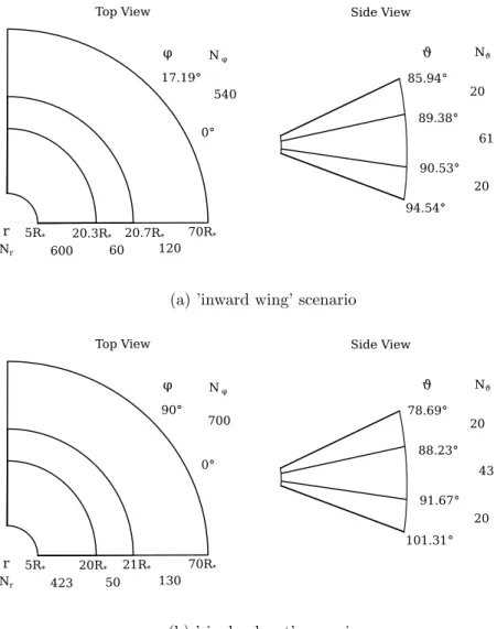
5.1.4 Grid Structures and Physical Parameters . . . . 58

5.2 Spatial Structure of the Steady-State Stellar Wind . . . . 61

5.3 Methods for the Wave Analysis . . . . 63

5.4 The Inward Going Alfv´ en Wing . . . . 64

5.4.1 Path in the Stellar Wind . . . . 64

5.4.2 Properties of the Wing . . . . 65

5.4.3 Energetics of the Alfv´ en Wing . . . . 67

5.5 The Outward Going Wave Structures . . . . 73

5.5.1 Wave pattern . . . . 73

5.5.2 Alfv´ en Wing . . . . 76

5.5.3 Slow Mode and Slow Shock . . . . 77

5.5.4 Wake . . . . 80

6 Wing-Wing Interaction 81 6.1 MHD Setup with Two Planets . . . . 81

6.2 SPI From Two Planets . . . . 82

6.3 Temporal Evolution of the Star-Planet Interaction . . . . 84

6.3.1 On Wave-Wave Interactions . . . . 84

6.3.2 Alfv´ en Wings Over Time . . . . 84

6.3.3 Compressional Waves Over Time . . . . 88

6.4 Implications for Time-Variability in SPI . . . . 89

7 The Effect of a Coronal Mass Ejection on SPI 91 7.1 Modelling CME and Planet . . . . 91

7.1.1 How to Align Planet and CME . . . . 92

7.2 The Stellar Wind with a CME . . . . 93

7.3 Time-Variable Wave Pattern . . . . 95

7.3.1 The Alfv´ en Wing at Ingress . . . . 96

7.3.2 The Alfv´ en Wing at Egress . . . . 98

8 Flare Triggering at TRAPPIST-1 101 8.1 Observability of SPI . . . 101

8.2 Flares at TRAPPIST-1 . . . 102

8.3 Analysis of the Flare Time-Series . . . 102

8.3.1 Giving Flares a Duration . . . 102

8.3.2 Fourier Analysis and Autocorrelation . . . 103

8.3.3 Significance Tests . . . 104

Contents

8.4 Triggered Flares at TRAPPIST-1? . . . 106

8.4.1 Fourier Spectra and Autocorrelation . . . 106

8.4.2 Null Hypothesis . . . 107

8.4.3 Artificial Triggering Signals . . . 108

8.5 Visibility of Triggered Flares at TRAPPIST-1 . . . 114

9 Conclusions 117

Bibliography 121

Research Data Management 141

Acknowledgements 143

Eidesstattliche Erkl¨ arung 145

1 Introduction

Electromagnetic Star-Planet Interaction (SPI) describes the coupling between plan- ets and their host stars via the stellar magnetic field. This type of coupling does not exist between the Sun and its planets. Therefore, research has to rely on other stellar systems, where the planets are much closer to their star. Accordingly, the field of star-planet interaction is relatively young, like all fields of exoplanet research. Cuntz et al. (2000) and Rubenstein and Schaefer (2000) were the first who proposed that electromagnetic coupling between planets and their stars may enhance the stellar activity. Shkolnik et al. (2003) claimed the first detection of SPI in a system called HD 179949. Soon afterwards, first MHD modelling studies simulated SPI (Ip et al., 2004; Preusse et al., 2005).

The coupling between planet and star establishes via Alfv´ en waves that move from the planet to the star and carry energy (Neubauer, 1980; Saur et al., 2013).

However, the stellar wind accelerates with distance from the star, and the Alfv´ en speed reduces with distance. Therefore, at some point, the wave speed is lower than the wind velocity and the waves cannot travel upstream towards the star anymore. All solar system planets lie outside this so-called Alfv´ en radius, which is the reason why there is no SPI in the Solar System.

In our solar system, we have the well studied analogous phenomenon of moon- magnetosphere coupling. The prime example of moon-magnetosphere coupling is the interaction between Jupiter and its moon Io. This interaction generates bright auroral spots in Jupiter’s ionosphere (Clarke et al., 1996; Clarke et al., 2002), also called auroral footprints. First hints for an interaction between Jupiter and Io came from radio observations (Bigg, 1964), followed by in-situ observations with Voyager (Acuna et al., 1981), observations in the infrared (Connerney et al., 1993) and the UV with the Hubble Space Telescope (Clarke et al., 1996).

All observations of the footprints have in common that one can spatially resolve the footprint. Something like that is not (yet) possible in the case of star-planet interaction, which makes it challenging to distinguish related emissions. Observa- tions become especially difficult because stars themselves are very luminous and variable. Therefore, current observational approaches often concentrate on cer- tain wavelength ranges to better resolve excess emissions. Typical examples are the chromospheric Ca II K and H lines (Shkolnik et al., 2003), enhanced coronal X-ray emissions (Saar et al., 2008) or the radio range (Zarka, 2007). However, in addition to difficulties with spatial resolution, we have no evidence about the wavelengths that SPI may excite. That makes spectral observations somewhat prone to misinterpretations. Observations, therefore, require additional indicators that point at a planetary origin of the observed emissions.

One possibility that can show a connection between stellar emissions and planets

are temporal variabilities in the strength of the SPI. Evidence of certain period-

icities that can only appear from an interaction between planet and star help to

identify SPI in stellar signals. Such an approach was applied by Shkolnik et al.

(2003). The authors identified a short sequence of signals in observations of HD 179949 that appears with the orbital period of the close-in planet. However, the possible range of periods is much larger than the pure orbital period of the planet.

In this work, we will, therefore, present and investigate different mechanisms that cause temporal variability in SPI.

To provide a comprehensive overview of the whole topic of star-planet interaction, we present the current state of research in chapter 2. The chapter comprises general introductions towards exoplanets and stars. On that basis, we will introduce the TRAPPIST-1 system. Due to its seven terrestrial planets in close orbit around the star (Gillon et al., 2016, 2017) it is an exciting target for the research of SPI.

At the end of the chapter, we will introduce the state of research about star-planet interaction and moon-magnetosphere interaction.

In chapter 3, we introduce the necessary theory for our studies. That involves MHD wave theory, the applied analytic stellar wind model based on Parker (1958) and theory towards sub-Alfv´ enic interaction based on Neubauer (1980) and Saur et al. (2013). In section 3.4, we present our contribution to the concepts of SPI, with the characterisation of four different mechanisms for time-variable SPI.

Chapter 4 presents the results of the semi-analytic parameter study. The chapter aims to find out if TRAPPIST-1 is a suitable candidate for the search for SPI.

Additionally, we determine the expected strengths of SPI.

In chapter 5, we present our MHD model setup to simulate time-variable SPI. We perform an extensive analysis of the wave structures that belong to star-planet interaction. Additionally, to the effects described in chapter 5, we analyse two additional scenarios that require full time-dependence of the model. The first one involves the planets TRAPPIST-1 b and c, which we simulate to investigate their mutual electromagnetic interaction. chapter 6 presents the respective time- dependent results. The final subject of MHD modelling investigates how a coronal mass ejection affects SPI (chapter 7).

The last part of our results in chapter 8 deals with the analysis of flares observed in the TRAPPIST-1 system. We present the results of the Fourier transform and the autocorrelation that are published in Fischer and Saur (2019). Additionally, we perform statistical tests to determine the significance of the obtained results.

Finally, in chapter 9, we wrap everything up and conclude our findings.

2 Exoplanets, Stars and their Interaction - The State of Knowledge

In this chapter, we will introduce the reader to the current state of knowledge about Star-Planet Interaction (SPI) and the main target of our studies, the TRAPPIST-1 system. However, first we will introduce exoplanets and stars with their respective properties.

2.1 What are Exoplanets?

Planets outside our solar system are called ’extrasolar planets’ or, more commonly,

’exoplanets’. Currently we know about 4141 confirmed exoplanets (NASA Exo- planet Archive, 26th March 2020). About 1254 planets have radii below two Earth radii and from these about 403 have radii smaller than 1.25 R

.

Our Solar System hosts eight planets, plus a large number of dwarf planets and moons. The Solar System planets have strongly influenced cultures and religions here on Earth and today they wear the names of ancient gods. About as much influence as our planets have on us, the stars we see in the night sky caught our interest and stimulated our imagination. The idea of unknown, inhabited worlds around other stars has even inspired modern popular culture. We still do not know whether we are alone in the universe or not, but for 25 years already, we know about the existence of planets outside our solar system (Mayor and Queloz , 1995).

In this section we will introduce exoplanets in general. We start with an overview of the different types of exoplanets. The question if we are alone or not is an important driver for the enormous interest in exoplanets. Therefore we will talk briefly about the topic of habitable zones and planets therein. Finally we address the most important detection methods for exoplanets.

2.1.1 Types of Exoplanets

A unified classification of exoplanets is yet to be established, as exoplanets show a

large variation in their properties. Possible characteristics for a classification are

for example size and mass, composition or orbital properties. However, the most

common classification is the one applied for the Solar System planets, which takes

size, mass and composition into account. This system typically divides planets

into the three classes of gas giants, ice giants and rocky terrestrial planets. In

the context of exoplanets, several subclasses appear due to the large variations of

their properties mentioned above. In this section we will introduce the three main

classes and their corresponding subclasses.

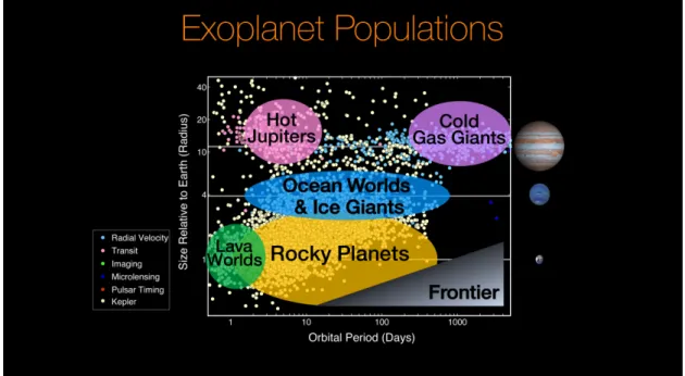
Figure 2.1: Exoplanet population as of August 2017 with sketched approxi- mate classification. (Credit: NASA/Ames Research Center/Natalie Batalha/Wendy Stenzel, https://www.nasa.gov/image-feature/

ames/kepler/exoplanet-populations).

Some of the typical classes and subclasses of exoplanets are sketched in Figure 2.1.

The figure shows a scatter plot of all detected exoplanets until August 2017 plotting the planet radius in units of Earth radii against the orbital period in days. For comparison Jupiter, Neptune and Earth are drawn at their respective position on the y-axis. Different classes of exoplanets are indicated by different shadings.

We will start with the gas giants. In Figure 2.1 those are the planets at the very top, shaded with red and purple. In the Solar System, Jupiter and Saturn belong to this class. Jupiter is often used as a default for gas giant exoplanets, much like Earth for the smaller, rocky planets. Gas giants represent the largest and heaviest planets that consist mostly of hydrogen and helium (Militzer et al., 2016).

Masses lie in the range between approximately 1 and 13 Jupiter masses. The lower mass boundary is not clearly defined, whereas the upper boundary represents the minimum mass where deuterium fusion sets in and the object is classified as a brown dwarf (Burgasser , 2008). From Jupiter and Saturn are expected to have a solid core (Militzer et al., 2016) and a thick layer of metallic hydrogen (Militzer et al., 2016). At Jupiter this layer is considered to extend from the core up to 0.85 R

(Connerney et al., 2018). This layer acts as Jupiter’s dynamo region and is responsible for the strong jovian magnetic field (Militzer et al., 2016). A subclass of gas giants are the so-called Hot Jupiters. Those planets are extremely close to their host stars, most of them with orbital periods of a few days (Figure 2.1), where strong stellar irradiation heats up the planets’ atmospheres. For comparison, Jupiter’s orbital period is 4330 days. The first detected and confirmed Hot Jupiter was the planet 51 Peg b (Mayor and Queloz , 1995).

The next smaller class of planets are the ice giants with an approximate radius of four Earth radii. In the Solar System Uranus and Neptune belong to this class.

Ice giants like Neptune consist largely of methane, ammonia and water (Hubbard

2.1 What are Exoplanets?

et al., 1991) and to lesser extent of hydrogen and helium, unlike the gas giants.

Therefore ice giants are expected to harbour thick layers of ice beneath a gaseous surface layer (Helled et al., 2020). To date most known planets of this kind are much closer to their host star than Uranus and Neptune are to the Sun. Among the ice giants, there two notable subclasses: Mini-Neptunes and Warm/Hot Neptunes.

The latter class, just like Hot Jupiters, are planets that are very close to their host star and receive high irradiation. The first class differs in size from the ice giants and poses a conflict with the terrestrial planets, which will be discussed later.

The smallest class are rocky planets, also called terrestrial planets. Rocky planets typically have small radii of R

< 2 R

. In our Solar System the inner planets Mercury, Venus, Earth and Mars belong to this class, as well as all dwarf planets, e.g. Pluto and Ceres. Planets in this class consist mostly of a solid planetary body and are silicate and metal rich. Their densities are therefore much larger than the densities of the bigger planet classes. Additionally, these planets can have gaseous envelopes in form of atmospheres or exospheres. The example of the Earth shows that planets can also have hydrospheres in form of oceans and a global water cycle. The icy moons of Jupiter and Saturn even have global oceans beneath their ice crust. Saturn’s moon Titan is an example of an alternative type of hydrosphere consisting of nitrogen and methane (Dermott and Sagan, 1995;

Tokano et al., 2006).

Terrestrial planets have radii up to two Earth radii, which is considered to be the boundary towards Mini-Neptunes (Fabrycky et al., 2014). A subclass of planets that may hypothetically exist at the boundary between Super-Earths and Mini- Neptunes are ocean planets (Kuchner , 2003; L´ eger et al., 2004). Those worlds would have a thick surface layer of water in contrast to Mini-Neptunes that would have an extended hydrogen rich atmosphere (de Mooij et al., 2012). Possible ocean planet candidates are GJ 1214 b (Charbonneau et al., 2009; Berta et al., 2012) and Kepler-62 e and f (Kaltenegger et al., 2013).

The hypothetical rocky-planet-analogue to Hot Jupiters are the so-called lava planets. While Hot Jupiters heat up due to intense irradiation from the star, lava planets are believed to be primarily heated by extreme tidal forces from the star (Henning et al., 2009). Recently Kislyakova et al. (2018) showed that magnetic induction in a planet embedded in a strong and variable magnetic field may cause internal heating that is comparable to Io’s tidal heating and may cause volcan- ism on a planet. A potential candidate for such a planet subclass is COROT-7b (Barnes et al., 2010).

2.1.2 Habitability

The search for extraterrestrial life is a major motivation for exoplanet research and strongly linked to the question of habitability. From the Solar System we know that by far not all planets support the evolution of life. In fact, life as we know it from Earth, requires very special conditions. Therefore this section is dedicated to the topic of planetary habitability.

The key concept behind the idea of planetary habitability is the habitable zone.

In astrophysics this zone is defined as the distance range around a star where

liquid water can exist on the surface of a terrestrial planet (Seager, 2013). Histor-

ically, the concept of a zone where the stellar irradiation affects the suitability of

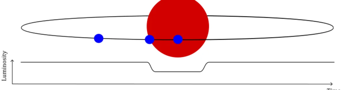
Luminosity

Time

Figure 2.2: Sketch of the principle concept behind the transit method.

a planet for life, has first been published by Huang (1959). Kasting et al. (1993) modelled the habitable zone for main sequence stars and planets with Earth-like atmospheres, consisting of CO

, H

O and N

. The planetary atmospheres ensure a stable temperature via a green house effect. The authors also describe a common extension of the habitable zone into a conservative and an optimistic habitable zone. In the conservative view, the inner edge of the habitable zone is deter- mined by the photolysis of water and the escape of hydrogen. The outer edge is determined by the formation of CO

clouds. Kasting et al. (1993) estimate the conservative habitable zone to be in the range between 0.95 AU and 1.15 AU.

The optimistic view extends the boundaries of the habitable zone. It is based on observations of Venus and Mars that indicate the presence of liquid water on both planets in the past. Kasting et al. (1993) estimate the solar radiation at the time of the presence of liquid water at both planets and conclude that early Mars re- ceived about 30% of today’s Earth’s radiation and recent Venus about 170%. The corresponding range extends from 0.75 AU to 1.77 AU. However, the estimation of the habitable zone varies due to several factors, especially the atmospheric com- position and the assumed effects of the greenhouse effect. Therefore other authors come up with different estimates.

The concept of the habitable zone is of major interest in astronomy, since the orbital distance of a planet can be observed. Actual habitability however is also affected by various other effects. Lammer et al. (2009) review those factors includ- ing geophysical processes, like plate tectonics, a dynamo process and accordingly the existence of a planetary magnetic field. A magnetic field shields the atmo- sphere of a planet from the stellar wind and more dangerous effects like flares and coronal mass ejections (Lammer et al., 2009). The authors also discuss the possibility of other types of habitats outside the habitable zone. The icy moons in our Solar System are known to harbour subsurface water oceans and therefore may be habitable. We know from Earth that early biotopes evolved around black smokers in the deep sea (Lammer et al., 2009).

2.1.3 Detection Methods

Here we will introduce common methods to detect exoplanets. The focus lies

on the two most important methods: the transit method and the radial velocity

method. The next best notable methods are gravitational microlensing and direct

imaging, but their contributions to the number of detections are small. There

2.1 What are Exoplanets?

are other methods as well, which are sometimes specialisations of the mentioned methods, but until today, their detection numbers are negligible.

2.1.3.1 Transit Method

The principle behind the transit method is fairly simple: A star emits light and if a planet is in front of the star it blocks some of the emitted light. Figure 2.2 shows a sketch of the situation. One sees a star and measure its luminosity as a function of time. This observation technique is called photometry and yields a so-called stellar light curve, which is sketched below the star. The sketch further depicts a planet at three different positions on its orbit around the star and the effect on the stellar light curve. At first the planet is not in front of the stellar disk and has no effect on the light curve. Later it passes the stellar limb and initiates its transit across the stellar disk, visible as a ramp of decreasing luminosity in the light curve. As soon as the planet is completely in front of the star the dip in the light curve reaches its maximum. This is called the transit depth. Later the planet moves out of the stellar path and one sees the full stellar luminosity again.

In general the transit method can provide information about the planet’s radius, the orbital period and, given the detector is sufficiently sensitive, also about the planetary atmosphere from absorption features. The Hot Jupiter HD 209458 b was the first planet, detected by the transit method (Charbonneau et al., 2000). The method also allowed to probe the planetary atmosphere. For example Charbonneau et al. (2002) reported the first ever exoplanet atmosphere and Barman (2007) found evidence for water vapour in the planet’s atmosphere.

The search for transits is more effective from space, because it avoids disturbing effects from Earth’s atmosphere. The first space telescope designed to search for exoplanets with the transit method was the french COROT-mission from 2006 to 2013. The most successful ’planet hunter’ to date is the Kepler space telescope.

It started in March 2009 to follow the Earth on a solar orbit. The mission was designed to observe a fixed field of view for several years and detect Earth-like planets at about 1 AU around sun-like stars. After the failure of two reaction wheels, the original mission could not be prolonged but instead, the field of view was shifted into the ecliptic and changed every 83 days. The new mission was named K2 and should find more short-period planets from 2014 to 2018. Borucki et al. (2010) reported the first results on short period transiting exoplanets ob- served by the Kepler-mission. Fressin et al. (2012) found the first Earth-sized exoplanet and Jenkins et al. (2015) found the first Earth-sized exoplanet in the habitable zone of a sun-like star. The first planet found by the K2-mission was HIP 116454 b (Vanderburg et al., 2015).

The NASA Exoplanet Archive lists 4141 exoplanets (23rd March 2020, as for the

following numbers of this paragraph) where 2348 have been discovered by Kepler

and 397 by K2. In addition both missions provided 3309 candidates that still have

to be confirmed. Therefore Kepler is also the main reason that the transit method

is the most successful method in detecting exoplanets so far. Kepler’s successor,

the TESS-telescope is currently in space (start 2018) and ends its primary mission

mid 2020.

2.1.3.2 Radial Velocity Method

Star

Planet

Figure 2.3: Physical principle behind the radial velocity method.

The radial velocity method bases on spectral variations of the stellar light. When a planet orbits a star, then both objects revolve around the mutual centre of mass. Figure 2.3 visualises the physics behind the idea. The black circles sketch the orbits of the stellar and the planetary orbits around centre of mass respectively, and the cross indicates the common centre of mass.

Due to the many times larger mass of the star, the stellar motion is weaker than the planetary motion. The stellar motion however causes a Doppler shift of the stellar radiation. If the star moves towards the observer there is a blue shift and when it moves away from the observer there is a red shift. Blue shift means that the light has a shorter wavelength and red shift implies a slightly longer wavelength.

The radial velocity method is the oldest method, dating back to the discovery of the Hot Jupiter 51 Peg b (Mayor and Queloz , 1995). Today giant planets further away from their star are detectable or close in rocky planets around small stars. An example for Jupiter-analogues is HD 154345 b (Wright et al., 2007; Boisse et al., 2012). An example for small planets around a Red dwarf is Proxima Centauri b (Anglada-Escud´ e et al., 2016)

2.1.3.3 Further Methods

There are a few more methods, which are not as successful as the methods de- scribed before. The most notable methods are gravitational microlensing and direct imaging.

Direct imaging is an approach to see an exoplanet directly. It typically requires a system close to our Solar System, where the planet is large and far away from its host star. In such a constellation one can distinguish the planet from the star.

Due to typical planetary temperatures the maximum of the emissions lies in the infrared wavelength range. An early finding is the planet 2M1207b (Chauvin et al., 2004), which orbits a faint brown dwarf at a distance of 55 AU. The planet is quite hot on its own due to gravitational contraction (Mohanty et al., 2007)

Gavitational microlensing bases on relativistic effects. It requires two stars to be aligned in the line of sight. The closer star acts as a lens for the star behind it. The stellar mass bends the light around it. If a planet orbits the star this generates an observable signal. The first planet to be detected by this method was OGLE-2003-BLG-235Lb by Bennett et al. (2006).

2.2 A Short Note on Stars

We saw before that there are a lot of planets in our universe. Also, a lot of stars

have at least one planet in an orbit around them. However, not all stars are like

our sun. Most of them have completely different properties. Common for all stars

2.2 A Short Note on Stars

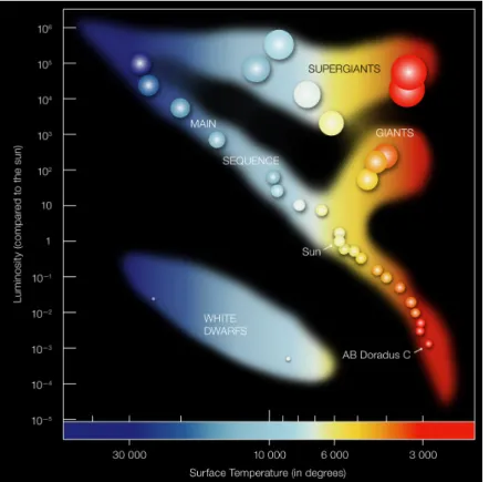
Figure 2.4: Hertzsprung-Russell diagram (Credit: ESO, https://www.eso.org/

public/images/eso0728c/).

is their main source of energy: hydrogen fusion, the so-called hydrogen burning.

This process fuses light hydrogen nuclei to the heavier helium nuclei and thereby releases energy (Hansen et al., 2004).

This section will have a closer look at stars and brown dwarfs. It introduces, which types of stars exist and how stars are commonly categorised. Afterwards, the stellar structure and stellar magnetic fields are presented. A special focus lies on M-dwarf stars.

2.2.1 Types of Stars and Spectral Classes

All known stars and brown dwarfs can be described by their position in the Hertzsprung-Russell diagram (HR diagram, Figure 2.4). The HR diagram draws the luminosity of a stellar object against the effective temperature, which typi- cally decreases in x-direction. The effective temperature is the temperature that a black body had to have to emit the same power as the star and is an indicator for the spectral class of a star. See Hansen et al. (2004) for further detail. Spectral classes represent a system to categorise stars according to their color and tradi- tionally include the classes O, B, A, F, G, K, M (from hot to cool stars). This system goes back to Morgan et al. (1943) and bases strongly on stellar absorption features (Hansen et al., 2004).

The HR diagram shows three big structures: The main sequence, the giant stars

and the White dwarfs. The most prominent of these structures is the main se-

quence (Figure 2.4) going from high effective temperatures and luminosities (ba-

sically upper left corner) to low temperatures and luminosities (lower right corner

of the diagram). The stars on the main sequence span the full range of spectral classes, which also represents the continuous decrease in stellar mass from O- to M-stars. Our sun is a star of spectral type G2. At the low-mass end of the stellar main sequence, there are the M-dwarfs. Those stars are also called Red dwarfs due to their reddish colour. Their mass lies below 0.3 M

(Hansen et al., 2004).

Not included in Figure 2.4 is the brown dwarf regime, which extends the main sequence on the low mass end. Brown dwarfs are commonly referred to as failed stars (Burgasser , 2008) because they never gained enough mass to ignite the fusion of hydrogen inside them. These objects are classified by the spectral classes M, L, T and Y, whereas the last three have been especially introduced for brown dwarfs (Mart´ın et al., 1999; McLean et al., 2001; Cushing et al., 2011).

Further notable populations according to the HR diagram are the White dwarfs and the giant stars. Giant stars are extremely luminous stars and lie above the main sequence. They evolve from sun-like main sequence stars that fused a certain amount of their hydrogen via the so-called proton-proton cycle (Hansen et al., 2004). At that phase the temperature inside the star became so high that the CNO hydrogen burning becomes increasingly important and causes the star to expand enormously (Hansen et al., 2004). The CNO cycle includes the heavy elements Carbon, Nitrogen, and Oxygen, to fuse hydrogen to helium. While giant stars represent a stage in the evolution of certain stars, white dwarfs are one of the three possible ways a star can end up after its ”death” (Hansen et al., 2004).

White dwarfs are the cores of giant stars that got rid of their outer shells after the end of nuclear fusion. For heavier cores, the star might end up as a neutron star or even a black hole. White dwarfs have a low luminosity compared to the main sequence, although they may have extremely high effective temperatures (Hansen et al., 2004).

2.2.2 Stellar Structure: Interior and Atmosphere

Just like planets, stars are stratified objects, with a certain internal structure that depends on the spectral class. The internal layers are mostly characterised by their role in energy production and transport. The Sun’s interior, for example, is structured into a convective core, a radiative zone and a convection zone. The core extends to about 0.3 R

and produces the majority of the stellar energy by fusion processes (Hanslmeier , 2007). In the radiation zone, heat transport happens by radiation. This zone extends up to about 0.6 R

(Hanslmeier, 2007). As the energy is transported outward, the temperature decreases with radial distance from the core. Hence, the base of the convective zone is the hottest part of the layer. The resulting temperature gradient drives convection processes. Over the main sequence, the internal stratification varies. In low mass stars for example, the convective zone increases its relative size with decreasing stellar mass M

. Low mass M-dwarfs with M

< 0.3 M

have fully convective interiors (Hansen et al., 2004).

Stars also have stratified atmospheres. The solar atmosphere is subdivided into photosphere, chromosphere, transition zone and corona (B¨ ohm-Vitense, 1989).

The photosphere is the lowest and densest part of the atmosphere (Eddy and Ise ,

1979). Its temperature lies, in case of the sun, at about 5000 K and is comparable

to the effective temperature. The chromosphere cools down on its basis to about

2.2 A Short Note on Stars 3800 K (Avrett , 2003) and rises up to the range of 10

K (Eddy and Ise , 1979;

Hanslmeier , 2007). The transition zone is characterised by an extreme increase in temperature towards the coronal temperature of 10

K (Eddy and Ise , 1979;

Hanslmeier , 2007).

The different atmospheric layers with their typical temperatures cause different types of emissions. Thermal emissions in form of visible light originate from the photosphere (B¨ ohm-Vitense , 1989). The chromosphere exhibits emissions from the Hydrogen Balmer lines, metallic emission lines and ultraviolet emissions (B¨ ohm- Vitense , 1989). Further upward, the extremely hot corona is the only source of stellar X-ray emissions (B¨ ohm-Vitense, 1989).

2.2.3 Stellar Magnetic Fields and related Phenomena

Stars are highly magnetised objects. Most features of our Sun, as the best analysed star we know, are of magnetic origin. The large-scale magnetic field undergoes a cycle of 22 years, where it changes its direction, together with the sunspots, as an indicator of magnetic activity, that vary with an 11 years cycle (Brun and Browning, 2017). Sunspots are formed by strong, small-scale magnetic fields that emerge to the solar surface. The magnetic field inhibits convection flows, which transport heat to the surface (Brun and Browning, 2017). Therefore, the corre- sponding region is cooler than the surrounding and appears as a dark spot. Due to the strong magnetic fields, groups of sunspots are sources of eruptive events like flares and coronal mass ejections (Brun and Browning, 2017; Toriumi and Wang, 2019). Magnetic effects are also believed to be the main drivers of atmospheric heating at stars (Brun and Browning , 2017).

Fully convective M-dwarf stars (M < 0.3M

) appear to have a different field geometry than more massive stars. Right at the boundary towards the fully con- vective regime, i.e. at spectral class M3.5 (Reiners and Basri , 2009), the field appears to change from toroidal to mostly axisymmetric poloidal field structures (Brun and Browning , 2017). Morin et al. (2010) report two categories of magnetic fields on M-dwarfs. One type of star with strong axisymmetric dipole fields and on the other hand stars with weak magnetic fields and a non-axisymmetric compo- nent. (Reiners and Basri , 2009) report, that the majority of magnetic flux is stored in small-scale magnetic structures. In general, field strengths and geometries of late M-dwarfs are difficult to detect, because of the stars’ faintness.

Flares are explosive phenomena, driven by small scale magnetic fields that can drastically enhance a star’s luminosity. The first such event was the so called Carrington event (Carrington, 1859), named by the scientist who described it first.

Until today, this flare is still among the most powerful flares that we know from our sun. The current standard model, the so called CSHKP-model, bases on the work of Kopp and Pneuman (1976) and has been extended since then. The name as well, since every important contributor’s initial letter has been added. The model assumes, that open magnetic field lines reconnect, to form closed magnetic loops on the star. The outflowing stellar wind produces a shock inside the looped field, which heats the plasma. The wind eventually extends the magnetic loops and creates a reconnection zone. Oppositely directed magnetic field lines reconnect and release magnetic energy. A plasmoid is released together with radiative energy.

For further details see the review from Shibata and Magara (2011). The details of

the reconnection process are not yet fully understood, so quite possibly, the name of the model has to be further extended in the future. A flare can cause emissions in all atmospheric layers, whereas they are most commonly observed in coronal X-ray ranges (Shibata and Magara , 2011). For a large event, even the photosphere might react and emit white light (Shibata and Magara , 2011). Flares typically have a duration on the order of 10

-10

s (Shibata and Magara, 2011) and erupt from active regions, like groups of starspots (Toriumi and Wang, 2019).

Coronal Mass Ejections (CME) are large scale phenomena that erupt large amounts of plasma from active regions on the sun. The mass, carried by CMEs, usually ranges between 10

and 10

kg and the material erupts with velocities of several hundred km s

(Chen , 2011). The review of Chen (2011) distinguishes between two types of CME, the so called narrow CME and the normal CME. The author describes narrow CMEs as elongated jet-like structures that move along open field lines. These CMEs are believed to be the result of reconnection between small-scale magnetic loops and open field lines. Thus, these CMEs are often accompanied by, what the author calls a compact flare. On the other hand, the so called normal CME, is the more common type of event. Normal CMEs have a leading struc- ture loop-like structure, followed by a dark cavity and a bright core (Chen , 2011).

As powerful eruptions of material into the interplanetary space, CMEs affect the Earth’s space weather and can cause damage on technical devices and power grids (Schwenn, 2006; Pulkkinen, 2007).

2.3 TRAPPIST-1

The studies of this thesis base on the example of the TRAPPIST-1 system, due to the large number of close-in planets with accordingly short orbital periods.

Therefore we will introduce the system in more detail and start with the stellar parameters and go on to the planets.

A short note on nomenclature: We usually apply the abbreviation T1x to indicate the planets. T1 stands for the star TRAPPIST-1 and the x is a placeholder for the letters b to h, depending on the planet.

2.3.1 The Star

TRAPPIST-1 is a star of spectral class M8. It is located at a distance of 39 light years in the constellation Aquarius. The star was first discovered during the 2MASS All Sky Survey, among other low mass stars (Gizis et al., 2000). By that time, the star was only known under its 2MASS-identifier 2MASS J23062928- 0502285. Burgasser and Mamajek (2017) determined the most probable age of TRAPPIST-1 to be 7.6 Gyr with an error range of 2 Gyr.

As an M8 low-mass star TRAPPIST-1 has a mass of 93 Jupiter masses M

and

a size of 84257 km or 1.18 Jupiter radii R

(Van Grootel et al., 2018). Earlier

observations by Gillon et al. (2016) indicated an even lower mass of 84 M

, which

made it an object quite close to the border of the Brown Dwarf regime. Gillon

et al. (2016) carried out optical spectroscopy and did not detect the 670.8 nm

lithium line. This finding implies that TRAPPIST-1 belongs to the very low mass

stars, instead of the Brown Dwarfs.

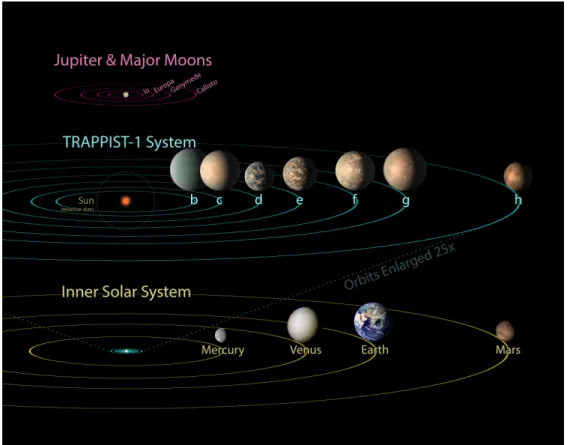
2.3 TRAPPIST-1

Figure 2.5: Comparison between Jupiter and its Galilean moons, the TRAPPIST- 1 system and the inner Solar System (Credit: NASA/JPL-Caltech).

The atmosphere of the star has an effective temperature of about 2500 K in the photosphere (Delrez et al., 2018). Observations in X-ray and UV ranges by Bourrier et al. (2017) and Wheatley et al. (2017) indicate the existence of a hot stellar corona and a moderately active Chromosphere.

The stellar rotation period T

has been somewhat controversial in the past. Early measurements by Reiners and Basri (2010) and Gillon et al. (2016) reported a rotation period of around 1 d. Luger et al. (2017) and Vida et al. (2017) then proposed T

to be 3.3 d based on photometric periodicities observed by K2. The latter is supported by Reiners et al. (2018) who conducted more precise radial velocity measurements and concluded a period of T

sin i > 2.7 d, whereas the inclination i is unknown. These new measurements are consistent with the rotation period obtained by Luger et al. (2017) and Vida et al. (2017). Recent observations by Hirano et al. (2020) showed that TRAPPIST-1’s spin axis is not tilted against the orbital planes of the co-planar planets.

2.3.2 The Planetary System

Gillon et al. (2016) announced the finding of three planets around the star, followed

one year later by Gillon et al. (2017) with the announcement of a total of seven

confirmed exoplanets around TRAPPIST-1. All planets are approximately Earth-

sized and in close orbits around their host star (Gillon et al., 2017). Up to four

of the planets may lie in the habitable zone of the star (O’Malley-James and

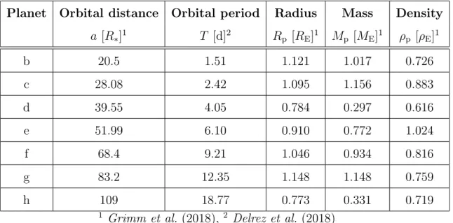
Table 2.1: Important parameters of the planets in the TRAPPIST-1 system, i.e.

orbital distance and period, radius, mass and the average planetary density.

Planet Orbital distance Orbital period Radius Mass Density a [R

]

T [d]

R

[R

]

M

[M

]

ρ

[ρ

]

b 20.5 1.51 1.121 1.017 0.726

c 28.08 2.42 1.095 1.156 0.883

d 39.55 4.05 0.784 0.297 0.616

e 51.99 6.10 0.910 0.772 1.024

f 68.4 9.21 1.046 0.934 0.816

g 83.2 12.35 1.148 1.148 0.759

h 109 18.77 0.773 0.331 0.719

1

Grimm et al. (2018),

Delrez et al. (2018)

Kaltenegger , 2017). These are the reasons that this system gained much fame over the past three years. Figure 2.5 shows an artists view of the TRAPPIST-1 system (middle) in comparison to Jupiter with its Galilean moons (top) and the inner Solar System with the terrestrial planets (bottom). The size of the Solar System is reduced by a factor of 25 to compare it to the TRAPPIST-1 system (centre, just around the Sun). In size, the TRAPPIST-1 system is comparable to the Jupiter system. However, the appearance of the planets is subject to the artist’s fantasy, as we do not know about it yet.

Table 2.1 lists the most important planetary parameters: semi-major axis a in stellar radii R

, the orbital period T in days, the planetary radius R

in Earth radii R

, the planetary mass M

in Earth masses M

and the according planetary density ρ

relative to Earth’s density ρ

. The planets orbit TRAPPIST-1 at distances between 20.5 and 109 stellar radii R

(Grimm et al., 2018) and have orbital periods between 1.5 days and 18.7 days (Delrez et al., 2018). According to Turbet et al. (2018), all planets could be tidally locked, i.e. their rotational period equals their orbital period. Luger et al. (2017) report that all seven planets are in orbital resonance. Orbital resonance is the phenomenon that orbital periods of celestial objects like moons and planets are integral multiples of each other.

All planets belong to the class of terrestrial planets with radii between 0.773 and 1.148 R

and masses between 0.297 and 1.156 M

. Planets d and h are quite similar in size and mass. The two planets are the smallest of the system. The planets b, c, and g are all slightly larger than Earth (up to 15%) and slightly more massive (up to 15% as well). However, the planetary density is quite low compared to Earth. Only planet e with 1.024 ρ

has a comparable density to Earth. All other planets range between 0.616 to 0.883 ρ

. All parameters have been estimated by Grimm et al. (2018).

The interior of exoplanets to date is unknown and our knowledge bases on model

2.4 State of Research about Electromagnetic Star-Planet Interaction estimates. A few studies have been conducted for TRAPPIST-1. Barr et al.

(2018) modelled possible interiors of all planets in the TRAPPIST-1 system and estimated the tidal heat flux present in all planets. The authors conclude that all planets may have significant amounts of water. Barr et al. (2018) note that T1b and c may experience sufficient tidal heating to sustain magma oceans in their mantles. Planets d, e, and f are expected to have tidal heat fluxes that are twenty times higher than Earth’s heat flux (Barr et al., 2018). Dorn et al. (2018) conduct a similar study based on statistical modelling. The authors estimated that the planets have water mass fractions between 0% and 25%. The water mass would contribute to the thickness of the gas envelope that the authors estimated to be up to 5% of the respective planetary radius. However, all authors agree that interior estimates vary heavily with the accuracy of the input data, especially when only mass and radius are available.

After the discovery of the planets, their atmospheres are now primary targets for further observations. Bourrier et al. (2017) observed TRAPPIST-1 in the Lyman- α. During the observations, the authors were able to observe the transits of T1b and c and found that the observed dimming was too large to be caused by the solid planet alone. According to Bourrier et al. (2017), the observations suggest the existence of hydrogen exospheres on both inner planets. These exospheres extend up to seven planetary radii and in the case of T1c into a comet-like tail.

De Wit et al. (2016) and de Wit et al. (2018) conclude from their observations that extended gas envelopes around all planets are unlikely. The authors do not expect that TRAPPIST-1’s planets have hydrogen-dominated atmospheres.

2.4 State of Research about Electromagnetic Star-Planet Interaction

Star-planet interaction (SPI) accounts for two major types of interaction: grav- itational and electromagnetic. Gravitational SPI typically involves gravitational effects that stars and planets exert on each other, e.g. tides and orbital motion.

The radial velocity method (section 2.1.3.2) is an example of how gravitational SPI is employed to detect planets. Electromagnetic star-planet interaction (in the following only SPI) is a quite young field compared to gravitational SPI. The main driver is the interaction between a planet and the surrounding stellar wind and magnetic field, which couples star and planet to each other.

In our Solar System, we have no such SPI because the planets are all too far away from the sun. However, in other stellar systems, this process can occur. Therefore, we will introduce the current state of knowledge towards electromagnetic SPI. In the following, we will further address the coupling between moons and planetary magnetospheres as the closest analogue to SPI. Afterwards, we will look at obser- vational evidence for SPI and will finally address theoretical models and numerical studies towards SPI.

2.4.1 The Situation in our Solar System

Moon-magnetosphere interaction (MMI) is the closest analogue to SPI that we

have in the Solar System. Historically, it is much older than SPI. In SPI-research,

the interaction between Io and Jupiter became a famous role model. However, many other large moons in the Solar System are known to generate MMI (Kivelson et al., 2007).

The earliest evidence for MMI date back to Bigg (1964), who observed Jupiter in the radio wavelength range and found that Io controls the jovian decametric radio emission. Goldreich and Lynden-Bell (1969) developed a model to explain the observations that assumed the absence of plasma, called the unipolar inductor model. The Pioneer 10 spacecraft, however, observed the presence of plasma in the Jupiter system, and especially a torus-shaped cloud of plasma in Io’s orbit (Frank et al., 1976). Volcanic activity on Io is the main source of torus plasma (Broadfoot et al., 1979). Goertz (1980) and Neubauer (1980) built upon these new findings and derived coupling models based on Alfv´ en waves. The model by Neubauer (1980) is the nowadays commonly applied Alfv´ en wing model. In-situ measurements during the flyby of the Voyager spacecraft (Acuna et al., 1981) and subsequently with the Galileo spacecraft (Kivelson et al., 1996a; Frank et al., 1996) verified the model.

Connerney et al. (1993) observed Jupiter in infrared wavelengths and detected auroral emissions that result from MMI between Jupiter and Io. Later on, the ul- traviolet wavelength range became the preferred wavelength range for observations of MMI, because the bulk of the emitted power lies in at UV wavelengths. Several authors performed observations of Io’s footprints with the Hubble Space Telescope (HST), e.g. Prang´ e et al. (1996); Clarke et al. (1996); Clarke et al. (2002); Bonfond et al. (2008) or Bonfond et al. (2012). Wannawichian et al. (2010, 2013) and Bon- fond et al. (2013) detected variations in the luminosity of the Io footprint. These variations come from the tilt in Jupiter’s magnetic field and result in a variable Poynting flux (Saur et al., 2013).

Io has also been subject in numerical modelling studies. Linker et al. (1988) analysed the occurring wave structures, i.e. Alfv´ en wings and Slow Mode waves.

Jacobsen et al. (2007) and Jacobsen et al. (2010) simulated the reflections of Io’s Alfv´ en wings at the boundary zones of the Io torus, which explain the occurrence of multiple auroral spots trailing behind the main footprint (Clarke et al., 2002).

Bl¨ ocker et al. (2018) studied the effect that a volcanic eruption on Io would have on the resulting MMI with an MHD model. The authors found that the volcanic plume locally enhances the strength of the interaction and result in a small Alfv´ en wing within the main wing, which they call Alfv´ en winglet.

The other three Galilean moons, Europa, Ganymede and Callisto, also host MMI (Kivelson et al., 2007). Callisto was, for a long time, only assumed to host MMI, because the respective auroral footprint lies within the main auroral oval and could not be detected (Clarke et al., 2002). Recently Bhattacharyya et al. (2018) published an analysis of HST data and claimed to have found Callisto’s footprint within Jupiter’s auroral oval.

The footprints of Europa (Clarke et al., 2002; Grodent et al., 2006) and Ganymede

(Clarke et al., 2002; Grodent et al., 2009) were detected and identified much earlier,

via HST observations. The identification of the spots was only possible because the

telescope could spatially resolve Jupiter. Ganymede is a unique example because it

is the only moon with an intrinsic magnetic field Kivelson et al. (1996b). Therefore,

Ganymede is the only magnetised planetary object that generates sub-Alfv´ enic

interaction. The interaction and the resulting Alfv´ en wings have been modelled

2.4 State of Research about Electromagnetic Star-Planet Interaction successfully with MHD models by, e.g. Jia et al. (2008, 2009) and Duling et al.

(2014).

Saturn’s moon Enceladus also forms a torus, just like Io (Dougherty et al., 2006).

The torus consists of material that originates from plumes of water and ice on Enceladus. Pryor et al. (2011) observed the footprints of Enceladus’ plasma in- teraction on Saturn. Prior to this finding Tokar et al. (2006) observed plasma interactions with Enceladus’ atmosphere and Saur et al. (2007) modelled the oc- curring sub-Alfv´ enic interaction.

2.4.2 Observations of Star-Planet Interaction

Observations of SPI are challenging, mostly because of the intense intrinsic lumi- nosity of the stellar hosts. Early suggestions for an observable relation between stars and planets date back to the year 2000. Cuntz et al. (2000) proposed a general increase in stellar activity, either by tidal interaction or by magnetic interaction.

Rubenstein and Schaefer (2000) made hot Jupiters responsible for the eruption of superflares on sun-like stars.

Claims of observational evidence for SPI exist for HD 179949 (Shkolnik et al., 2003; Shkolnik et al., 2005; Shkolnik et al., 2008) and υ And (Shkolnik et al., 2005;

Shkolnik et al., 2008). The authors observed enhanced Ca II H & K emission in synchronisation with the orbital period of the close-in planets. At HD 179949 the synchronisation has been observed in four of six observational epochs. Similar effects have been reported for υ And as well. Shkolnik et al. (2008) accounted for this on-off behaviour of the interaction by invoking a changing stellar magnetic field structure. However, Miller et al. (2012) showed that a chromospheric hot spot might mimic the existence of SPI at HD 179949 and υ And. Saar et al. (2008) observed a possible link between stellar X-ray emission and HD 179949 b. X-ray observations of υ And conducted by Poppenhaeger et al. (2011) provided evidence of activity linked to the stellar rotation but no connection to the planet.

Later observations followed the idea that SPI excites chromospheric Ca II H & K emissions. Walker et al. (2008) observed the star τ Boo A photometrically and in the Ca II K line. The star rotates tidally locked to its planet and features a variable region in advance of the planet that Walker et al. (2008) attributed to magnetic SPI. Staab et al. (2017) observed the system WASP-43 and likewise saw enhanced Ca II H & K emissions, which they attributed to the existence of SPI.

However, statistical analyses of several systems provide different results. Canto Martins et al. (2011) compares systems that have planets with semi-major axes a < 0.2 AU with stars that have no confirmed exoplanets. The authors saw no difference in the activity. Krejˇ cov´ a and Budaj (2012) see a difference between planet populations with semi-major axes a < 0.15 AU and a > 0.15 AU. The stars with close-in planets showed enhanced chromospheric activity and the others not.

Similarly to the chromospheric line emissions, analyses of X-ray emissions provide

different results as well. Miller et al. (2012) observed the system WASP-18 in

optical and X-ray wavelengths and saw no evidence for SPI. The authors claimed

WASP-18 b to potentially generate the strongest interaction among the known

planets at that time, based on planetary mass and semimajor axis. X-ray ob-

servations show that WASP-18 appears to be less active than expected from its

estimated age, which indicates a much weaker stellar magnetic field than in HD