Numerical simulations to assess the effect of urban heat island mitigation strategies on regional air quality.
Inaugural-Dissertation zur
Erlangung des Doktorgrades
der Mathematisch-Naturwissenschaftlichen Fakultät der Universität zu Köln
vorgelegt von
Joachim Fallmann
aus München
2014
Berichterstatter: Prof. Dr. Stefan Emeis
Prof. Dr. Michael Kerschgens
Datum der mündlichen Prüfung: 27.11.2014
“What place would you advise me to visit now?” he asked.
“The planet Earth,“ replied the geographer.
“It has a good reputation.”
And the little prince went away, thinking of his flower.
“The Little Prince”
Antoine de Saint-Exupéry
Zusammenfassung
II
Zusammenfassung
Die vorliegende Doktorarbeit präsentiert einen numerischen Modellierungsansatz um die Auswirkungen verschiedener Stadtplanungsmaßnahmen auf die Intensität der städtischen Wärmeinsel zu untersuchen und die Rückkopplung dieser Maßnahmen auf die chemische Zusammensetzung der städtischen Atmosphäre zu analysieren. Die Region Stuttgart dient dabei als Testgebiet.
Das mesoskalige Chemie-Transport-Modell WRF-Chem wird dazu verwendet, die Rückwirkung dieser Strategien zur Verringerung der städtischen Wärmeinsel auf die bodennahe Konzentration von primären (CO, NO, PM10) und sekundären Schadstoffen (Ozon) zu diskutieren.
Untersucht werden bekannte Vermeidungsmaßnahmen wie der Effekt heller Dach- und Fassadenflächen, städtische Begrünung oder die Veränderung der Bebauungsdichte. All diese Strategien bewirken eine Verringerung der städtischen Temperatur und tragen somit zur Reduzierung der Wärmeinsel bei.
Die Modellergebnisse zeigen, dass stark reflektierende Oberflächen die effizienteste Methode sind, die städtische Wärmeinsel zu reduzieren. Innerstädtische Begrünung und eine veränderte Bebauungsdichte zeigen geringere Effekte im Modell. Im Falle einer Erhöhung der Dachflächen-Albedo von 0.2 auf 0.7 wird eine Abnahme der städtischen Wärmeinsel um ca. 2 °C im Mittel erreicht.
Die Veränderung der Energie- und Strahlungseigenschaften der städtischen Oberflächen aufgrund der zuvor genannten Vermeidungsmaßnahmen wirkt sich unterschiedlich auf die chemische Zusammensetzung der Atmosphäre aus. Während die mittlere Ozon- Konzentration um ca. 5 - 8 % pro 1 °C Temperaturverringerung reduziert werden kann, wird ein Anstieg primärer Schadstoffe wie NO und CO um 5 - 25 % prognostiziert.
Primär wird durch die Abnahme der Temperatur die dynamische Struktur der Atmosphäre verändert. Die turbulente Durchmischung wird verringert, die Mischungsschichthöhe sinkt daher, wodurch die bodennahe Konzentration von direkt emittierten Schadstoffen wie CO und NO ansteigt. Für den Rückgang der Ozonkonzentration mit sinkender Temperatur ist in erster Linie die direkte Korrelation zwischen Temperatur und Reaktionsgeschwindigkeit verantwortlich.
Zusammenfassung
III Es muss jedoch beachtet werden, dass die Maßnahmen auch sekundäre Prozesse nach sich ziehen können. Eine Erhöhung der Oberflächenreflexion durch weiße Dächer zum Beispiel erhöht die Intensität der kurzwelligen Strahlung, was dazu führt, dass maximale Ozonkonzentrationen kurzzeitig sogar ansteigen können. Die Erhöhung biogener Emissionen aufgrund zusätzlicher Bepflanzung wird in dieser Arbeit nicht berücksichtigt.
Hauptresultat ist, dass der Einfluss von Maßnahmen zur Verringerung der städtischen Wärmeinsel auf die Dynamik größer ist als auf die Chemie. Während in bisherigen Studien vorwiegend die positive Auswirkung auf Ozonbelastung diskutiert wurde, untersucht diese Arbeit eine umfassende Luftchemie und arbeitet damit den negativen Effekt auf primäre Schadstoffe heraus.
Abstract
IV Abstract
Work in this thesis demonstrates a numerical modelling approach to analyse the effect of urban planning strategies on the urban heat island (UHI) intensity and further the feedback on the chemical composition of the urban atmosphere. The urban area of Stuttgart acts as test bed for the modelling.
The mesoscale chemical transport model WRF-Chem is used to investigate the effect of these urban heat island mitigation strategies on the surface concentration of primary (CO, NO, PM10) and secondary pollutants (O3).
Known mitigation strategies such as bright roofs and façades, urban greening and modification of the building density are in the focus. All these measures are able to reduce the urban temperature and thus mitigate urban heat island intensity.
Model results reveal that the most efficient way to cool down urban areas is the increase in the surface reflectivity. Changing the building albedo in the model from 0.2 to 0.7, lead to a reduction of the urban heat island by about 2 °C. The effect of urban greening and decreased building density is less.
The mitigation strategies which have been mentioned before promote changes in energetic and radiative properties of urban surfaces modifying the chemical nature of the urban atmosphere with regard to both primary and secondary compounds. A temperature reduction of 1 °C leads to an increase of NO and CO by 5-25 %, whereas the mean ozone concentration is projected to decrease by 5-8 %.
Reduced temperature on the surface and in the urban canopy layer influences the dynamical structure of the atmosphere, which leads to a reduction in turbulent mixing. The depth of the mixing layer is decreased accordingly. As a result, an increase of the near surface concentration of primary compounds is projected. Additionally, temperature directly controls the reactivity of chemical reactions, which explains the reduction of ozone concentration.
It has to be pointed out however, that different measures can generate secondary effects.
The increased portion of short wave radiation due to a reflexion from white roofs for instance can promote photochemical reactions, leading to an increase of peak ozone levels
Abstract
V although temperature has been reduced. The additional emission of biogenic compounds coming along with urban greening is not covered in this work.
The main result of this work indicates the dominating role of atmospheric dynamics when analysing the impacts of urban heat island mitigation strategies on urban air quality.
Whereas in earlier studies the main effort had been put on the positive effect of temperature dependent reduction of urban ozone concentration, this work analyses a complete air chemistry, being able to show negative effects on primary compounds like CO, NO and PM10 as well.
Acknowledgements
VI
Acknowledgements
First of all I have to thank my supervisor Prof. Dr. Stefan Emeis who supported me throughout the last 3 years. He introduced me to the field of meteorology and atmospheric modelling and gave me the opportunity to independently work on an interesting topic with public relevance.
Further I have to thank all members of the working group Regional Coupling of Ecosystem-Atmosphere Processes, in particular Renate Forkel, Richard Foreman and Peter Suppan who always had an open door for discussions and conversation of any kind.
Thanks also to Elija Bleher who supported me in my work as PHD-Representative of the IMK-IFU and to Michael Warscher who shared this position with me.
Thanks to Dr. Ulrich Reuter, Rainer Kapp and Dr. Rayk Rinke from the Department of Environmental Protection Stuttgart for the excellent teamwork and sharing of data and to Hugo Denier van der Gon (TNO) for chemical input data. This work was funded by EU- Project 3CE292P3 – ‘UHI - Development and application of mitigation and adaptation strategies and measures for counteracting the global UHI phenomenon’, implemented through the CENTRAL EUROPE Programme, co-financed by the ERDF. I like to thank all colleagues from NOAA in Boulder, CO, especially Dr. Georg Grell who let me join his working group for four months. Many thanks to the Mathematisch-Naturwissen- schaftlichen Fakultät der Universität zu Köln, in particular to Prof. Dr. Michael Kerschgens for giving me the opportunity to obtain my PHD from the faculty. The membership within the KIT Graduate School for Climate and Environment (GRACE) gave me extra financial support and advanced training opportunities.
Special thanks to Katja, Matthias, Janina, Carsten, Fabi, Andi, Benni, Tom, Ula, Petra etc.
for the informal everyday meetings and Marco, Ling and Mia for a great time in Boulder.
Thanks to the band members of DaGapo, the IFU-Football team and everybody in the institute who shared conversations with me.
Last but not least I thank my family and friends who supported me during the whole period of my PHD. Any time, they acknowledged my work and encouraged me to carry on. My parents, brother and sisters, who offered me all the support I needed and my friends Thomas and Philipp who have been around me since the early school years.
VII
Table of Contents
VIII
Table of Contents
Zusammenfassung II
Abstract IV
Acknowledgements VI
Table of Contents VIII
Acronyms XI
Notation XIII
List of Figures XV
List of Tables XX
1. Introduction 1
2. Global Background 6
2.1 Climate Change………... 6
2.2 Population growth and urbanization………... 8
2.3 Energy consumption and air quality………... 9
3. The Urban Climate 10 3.1 Introduction………... 10
3.2 Urban heat island characteristics………... 13
3.3 Energetic basis of the urban atmosphere………... 15
3.4 Strategies to mitigate UHI formation……… 20
3.4.1 Highly reflective roofs………. 20
3.4.2 Urban greening……… 21
3.4.3 Building geometry……… 22
3.4.4 Anthropogenic heating………. 25
Table of Contents
IX
4. Urban air quality 26
4.1 Photochemical formation of tropospheric ozone (O3) and the NOx-family……… 28
4.2 Carbon monoxide (CO)……… 33
4.3 Aerosols……… 34
4.4 Temperature dependence of chemical reactions……… 36
5. The model test bed 39 6. The WRF model 41 6.1 Urban mesoscale modelling………. 43
6.1.1 Basic Concept of SLUCM in WRF………. 46
6.1.2 Basic concept of BEP in WRF………. 48
6.2 Setting up WRF for real data application………. 51
6.2.1 Input data………. 51
6.2.2 Processing an urbanized WRF run………... 56
6.2.3 Sensitivity study……….. 59
6.2.4 Mitigation Scenarios……… 62
6.3 Basic configuration of WRF-Chem……….. 63
6.3.1 Initialization of the new land use data in WRF-Chem………. 64
6.3.2 Chemical initial conditions using the MACC emission inventory………... 67
6.3.3 Boundary conditions from MEGAN biogenic emissions………. 70
6.3.4 Global chemical boundary conditions using MOZART……….. 71
6.3.5 Evaluation……… 72
7. Results 75 7.1 Modelling of the Urban Heat Island (UHI) using WRF……… 75
7.2 Air Quality modelling with WRF-Chem……… 84
7.2.1 Chemical features of the urban atmosphere………. 84
7.2.2 Urban-rural circulation patterns……… 89
7.3 Effect of urban planning scenarios on UHI and chemical composition……… 92
7.3.1 WRF: Effect of urban design on UHI………... 92 7.3.2 WRF-Chem: Effect of urban planning strategies on chemical composition .99
Table of Contents
X
8. Discussion 104
8.1 Effects of reduced temperature on atmospheric dynamics……….. .104 8.2 Effects of temperature and radiation on chemical reactivity……… 107 8.3 Hourly budgets to quantify the impact on chemical composition………. .. 111
9. Conclusions 113
Appendix 116
Bibliography 128
Erklärung 137
Acronyms
XI Acronyms
AR Assessment Report
BEP Building Effect Parameterization
CBD Central Business District
CBL Convectively-driven Boundary Layer
CCN Cloud Condensation Nuclei
CFL Courant-Friedrichs-Levy
CFL Constant Flux Layer
CPU Central processing unit
DEM Digital Elevation Model
DESIREX Dual-use European Security IR Experiment 2008
DW Downwind
ECMWF European Centre for Medium Range Weather Forecast
EEA European Energy Agency
ERA European Reanalysis
ERDF European Regional Development Fund
GAINS Greenhouse Gas - Air Pollution Interactions and Synergies GMES Global Monitoring for Environment and Security
GDP Gross Domestic Product
HPC High performance cluster
IEA International Energy Agency
IPCC Intergovernmental Panel on Climate Change
LSM Land Surface Model
LAI Leaf Area Index
MACC Monitoring Atmospheric Chemical Composition MEGAN Model of Gases and Aerosols from Nature
MOST Monin-Obukhov Similarity Theory
MOZART Model of Ozone and Related Chemical Tracers
NOAA National Oceanographic and Atmospheric Administration
NWP Numerical Weather Prediction
OECD Organisation for Economic Co-operation and Development
Acronyms
XII
OPE Ozone Production Efficiency
PBL Planetary Boundary Layer
PDF Probability Density Function
PET Physiological Equivalent Temperature
PFT Plant Functional Type
RADM Regional Acid Emission Module
RANS Reynolds Averaged Navier Stokes Equations
RCP Representative Concentration Pathway
SIA Secondary Inorganic Aerosols
SLUCM Single Layer Urban Canopy Model
SNAP Standardized Nomenclature for Air Pollutants
SOA Secondary Organic Aerosols
SRES Special Report on Emissions Scenarios
SVF Sky View Factor
TKE Turbulent Kinetic Energy
TNO Netherlands Organisation for Applied Scientific Research
TOA Top of the atmosphere
TSP Total suspended particulate matter
UBL Urban Boundary Layer
UCL Urban Canopy Layer
UCM Urban Canopy Model
UHI Urban Heat Island
UHII Urban Heat Island Intensity
UN United Nations
URL Urban Roughness Layer
USGS US Geological Survey
UW Upwind
WHO World Health Organization
WRF Weather Research and Forecasting Model
WW2 World War 2
Notation
XIII Notation
A empirical pre-exponential parameter [cm3 molecule-1s-1]
α albedo [%]
c heat capacity[J kg−1 K−1]
ɛ emissivity [%]
E emission for one grid cell [mol km-2h-1]
GZ ground heat flux [Wm-2]
H building height [m]
H sensible heat flux [Wm-2]
HG sensible heat flux ground [Wm-2] HW sensible heat flux wall [Wm-2]
hν quantum energy [J]
ϴ solar incidence angle [°]
ϴ potential temperature [°C]
HWall heat flux wall [Wm-2]
HGround heat flux ground [Wm-2]
i general subscript
j general subscript
k general subscript
λ thermal conductivity [W m−1 K−1]
λ emission activity factor [-]
λCE canopy environment emission activity factor [-]
λage leaf age emission activity factor [-]
λSM soil moisture emission activity factor [-]
L* net long wave radiation at the surface [Wm-2] L↓ downward net long wave flux [Wm-2]
L turbulent length scale [m]
Q* total incoming solar radiation [Wm-2]
QF anthropogenic heat [Wm-2]
QE latent heat [Wm-2]
QH sensible heat [Wm-2]
ΔQS heat storage [Wm-2]
Notation
XIV
Qtotal total energy from canyon [Wm-2]
Qwall total energy from wall [Wm-2]
Qfloor total energy from floor [Wm-2]
ρ density [kg m−3]
ρiso canopy loss and production factor R ideal gas constant [J K-1mol-1] rs stomata resistance [sm-1]
rm mesophyll resistance representing [sm-1]
rlu resistance of the outer surfaces in the canopy [sm-1] rdc deep canopy resistance [sm-1]
rlc lower canopy resistance [sm-1] rac canopy height resistance [sm-1] rgs ground surface resistance [sm-1] σ Boltzmann constant [Wm-2K-4] SR incoming solar radiation [Wm-2] SD direct radiation [Wm-2]
SQ diffuse radiation [Wm-2]
SF scaling factor [-]
∆T(u-r(max)) maximum urban heat island [K]
Ts surface temperature [K]
Twall wall temperature [K]
Ttotal total temperature [K]
V volume of air in a grid cell [m³]
W building width [m]
Δx grid spacing [m]
Ψs sky view factor [-]
Ψw wall view factor [-]
ω area average factor [-]
z height [m]
ZR building height [m]
List of Figures
XV List of Figures
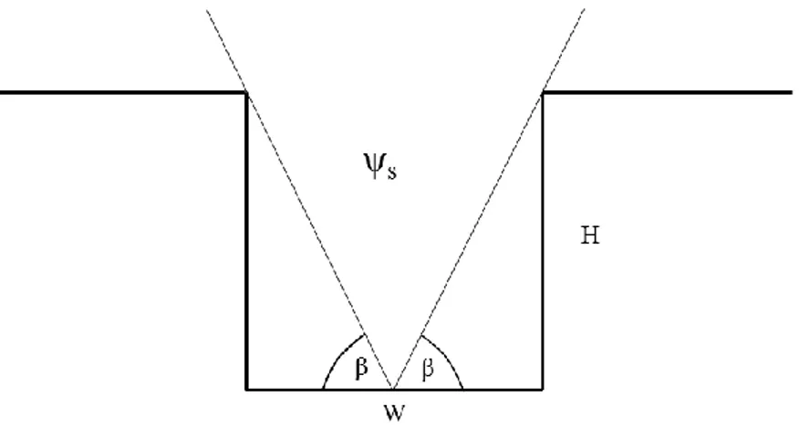
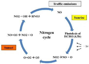
Fig. 1: Projected temperature (left) and CO2 (right) increase for each RCP Scenario (Stocker et al. 2013) ... 7 Fig. 2: Interactions across scales in atmospheric modelling (Britter & Hanna 2003) ... 11 Fig. 3: Urban environments in atmospheric processes across a range of scales (Oke 1987) ... 13 Fig. 4: Contour lines of equal UHI Intensity (EPA 2013) ... 14 Fig. 5: Schematic of the vertical layering of the urban boundary layer (UBL). H represents the average building height, p+ and p- indicate atmospheric pressure disturbances upstream and downstream of buildings (redrawn from Emeis 2010) ... 16 Fig. 6: Urban plume downwind of a large city (redrawn from Emeis 2010) ... 19 Fig. 7: Typical evolution of the atmospheric boundary layer as explained in Stull (1988) 19 Fig. 8: Sky view factor in a symmetrical street canyon described by its width (W) and its height (H), ψS = cos β (Oke 1982b) ... 23 Fig. 9: Diurnal nitrogen cycle producing and removing ozone in urban areas (Seinfeld &
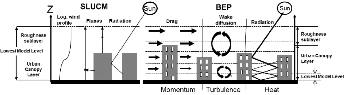
Pandis 2012) ... 32 Fig. 10: Reactions involving the HOx family in CO oxidation ... 34 Fig. 11: Mass and number distribution of urban particles with their typical source contribution (Seinfeld & Pandis 2012) ... 35 Fig. 12: Results from the box model according to the effect of increasing temperature on ozone (a) and HCHO (b) as well as the effect of rising isoprene levels (c) and relative humidity on ozone concentration (d). ... 38 Fig. 13: Land surface temperatures (LST) retrieved from LANDSAT7 radiative temperatures for September 19th 2005 10 am showing distinct temperature patterns throughout the urban area of Stuttgart. ... 40 Fig. 14: 2m air temperature for September 19th 2005 10 am for an urban (Stuttgart Schwabenzentrum) and a rural (Echterdingen) measurement station (left), and LST for the transect from Fig. 13 ... 40 Fig. 15: Schematic figure of the Single Layer Urban Canopy Model (Kusaka 2001) (left) and the multi-layer model: Building Effect Parameterization (Martilli 2002) right. These differ in representing the processes in the urban canopy layer (Chen 2011) ... 46 Fig. 16: Urban area of Stuttgart (200 km²) before (left) and after land use transformation.
The white circle indicates the central urban grid cell used for evaluation and sensitivity tests. ... 52 Fig. 17: Aerial photography showing as low density residential 31 (left), high density residential 32 (middle) and industrial/commercial 33 (right) (Source: Google Earth) ... 52 Fig. 18: Building heights extracted from high resolution DEM resolving every building height for one of the 3 defined urban classes according to the LUBW (2014) dataset: 31:
List of Figures
XVI
low density residential (a), 32: high density residential (b), 33: industrial/commercial (c) and all three land use classes combined. (Geobasisdaten © Landesamt für Geoinformation und Landentwicklung Baden-Württemberg, www.lgl-bw.de, Az.: 2851.9-1/19) ... 53 Fig. 19: Topographical input data used for WRF at the highest resolution of 1 km (30s).
The extent does not correspond to the actual domain size (left). The topography as displayed only for the urban area of Stuttgart (right) ... 56 Fig. 20: Model domains 1,2,3 for the WRF run projected to UTM WGS84 Europe Zone 32N ... 57 Fig. 21: Comparison between measured and observed 20 m potential temperature (upper three plots) and 20 m wind speed using BEP (left), SLUCM (middle) and the Bulk approach (right). Measurement station ‘Stuttgart Schwabenzentrum’ is located in the centre of the innermost domain and the centre of the urban area of Stuttgart. Model output is retrieved for the central urban grid cell as pointed out in Fig. 16. ... 59 Fig. 22: Comparison between radiosonde data and WRF output at ‘Stuttgart Schnarrenberg’ for August 13 2003 1200 h. Dry (a) and humid air temperature (c) are compared. Scatter plots show the correlations for TC (b) and TD (d) ... 60 Fig. 23: Observed (blue) and modelled (red) horizontal wind speed at ‘Stuttgart Schnarrenberg’ on August 13 2003 1200 h (a) and scatter plot comparing the two data sets (b) ... 61 Fig. 24: Simulated vertical profiles for actual temperature (a-b) and horizontal wind speed (c,d) at noon August 13 2003. The plots concentrate on the first 100 m including the urban canopy height indicated by maximum (dark dotted line) and mean building height (light dotted line). ... 61 Fig. 25: Resistance schematic for dry deposition model of Wesely (1989) ... 66 Fig. 26: MACC NO emissions for a weekday in August 2003 2000 h. Urban agglomerations can clearly be distinguished by road tracks (yellow, red) ... 69 Fig. 27: Urban area of Stuttgart (Source: Google Earth) with meteorological and air quality measurement stations (red dots). The square in the middle indicates the WRF-Chem grid cell of 9 km² used for evaluation of the chemical model runs. For comparison, a mean of 3 stations (blue dots) is calculated. ... 72 Fig. 28: Average daily trend of modelled concentration at an urban grid cell using the multi-layer approach (red) and the simple bulk approach (grey) in comparison to the mean of equivalent observations from 3 measurement stations located within that pixel (Fig. 27).
From left to right: Ozone (a), NO (b), NO2 (c), NOx (d), CO (e) and PM10 (f). ... 73 Fig. 29: Potential 2 m air temperature displayed for the innermost domain with Stuttgart in the centre (black outline). Four plots indicate the course of the day (August 13 2003), from left to right showing midnight, morning, solar noon and early evening hours. Light blue lines indicate the surface pressure. Dotted line in the rightmost figure indicates the cross section used for further analysis. White dots indicate the urban and rural grid cell used for the vertical profiles. ... 76 Fig. 30: Urban Heat Island intensity for the modelling period Aug 11-Aug 17 2003 calculated from the differences in 2 m potential temperature for an urban and a rural grid cell (a) and diurnal development of urban and rural temperature for Aug 13 2003 (b) ... 77
List of Figures
XVII Fig. 31: Surface plots showing skin temperature (left), potential 2 m temperature (middle) and 55 m potential temperature (right) for Aug 13 2003 2000 h ... 77 Fig. 32: West-East cross-section (Fig. 29) of temperature in 4 model levels 5m, 15m, 50m and 200m through the centre of the urban area of Stuttgart following the prevailing wind direction (west). Vertical profile of potential temperature over an urban and a rural grid cell (Fig. 29) is shown on the right (b) ... 78 Fig. 33: Vertical profiles of potential air temperature for an urban and a rural location (grid cell) on August 13 2003 at 0000 h, 1200 h and 2000 h – displayed are the first 2000 m (upper plots) and a closer look at the first 100 m (lower plots). The dotted lines in the lower plots indicate the maximum and mean building height of around 35 m and 8 m, respectively. The green line stands for the adiabatic temperature decrease. ... 79 Fig. 34: Vertical profile of horizontal wind speed for the first 2000 m (upper plots) and the first 100 m (lower plots) for the rural (dashed) and the urban (black) grid cell presented in Fig. 29. Maximum (black dashed line) and mean building height (grey dashed line) are added to the plot. Plots are generated for Aug 13 2003 0000 h, 1200 h and 2000 h ... 80 Fig. 35: Horizontal cross section of the wind component in vertical direction through the city centre of Stuttgart (black bar). Positive values (grey shading) indicate uplift. White shading indicates negative (downdraft) or zero values. Results are displayed for Aug 13 2003 2000 h As vertical wind speeds show considerably low values, they are presented in cm s-1 here. The red bars indicate the simulated height of the PBLH, the black shading represents the topography ... 81 Fig. 36: Mean wind directions at canopy height (33 m) in the city centre averaged over the modelling period presented for daytime (a) and night-time (b) situations. The topography is displayed on the right (c). ... 82 Fig. 37: Diurnal course of latent (LH) and sensible (SH) heat flux from an urban and a rural location (left) and Bowen ratio calculated from SH/LH presented for the model domain at 6 pm. Both plots present results for Aug 13 2003 ... 83 Fig. 38: Diurnal trend of near surface concentrations of NO, NO2 and Ozone for an urban grid cell for a selected day (August 13 0000 h – August 14 0600 h) ... 86 Fig. 39: Correlation between near surface concentrations of NO2 and ozone (a) and NO and ozone (b) for hourly model output of the modelling period (Aug 09 - Aug 17 2003). ... 87 Fig. 40: Vertical profile of ozone concentrations (a) for the same urban grid cell than analysed in Fig. 38 at four different times of the day (Aug 13 2003). Horizontal arrows indicate the direction of the shift in ozone concentration. O3 concentrations for 3 different times during the night for an urban and a rural location upwind of the city (b). ... 87 Fig. 41: Vertical profiles of urban CO NOx and O3 retrieved from WRF-Chem model output for August 13 2003 and three points in time (0800 h, 1500 h, and 2200 h). For each compound, an atmospheric column of 2000 m (a-c) and 100 m (d-f) is displayed for a central urban grid cell ... 88 Fig. 42: Distribution of all modelled wind directions in a height of 10 m of hourly WRF- Chem output with regard to the modelling period Aug 09 - Aug 17 2003 (a) and topographical map (WRF output) of the modelling area with location of the grid cells (white dots) used for the illustration of urban-rural circulation patterns (b) ... 89
List of Figures
XVIII
Fig. 43: Concentration of NOx, CO and O3 averaged over the time period Aug 09-Aug 17 2003. 3 vertical levels (10m, 33m and 55m) are displayed for an urban location (Urban) and two rural locations - one upwind (NW) and the other one downwind (SE), both with a distance of about 20 km to the urban centre. Values are retrieved from the WRF-Chem
‘Control Run’. Locations of grid cells are shown in Fig. 42b. ... 90 Fig. 44: Night and daytime concentrations of NOx, CO and ozone (O3) averaged over the time period Aug 09 - Aug 17 2003 for an urban location and two rural locations - one northwest (NW) and the other one southeast (SE), both with a distance of about 20 km to the urban grid cell (Fig. 42). Values are retrieved from the WRF-Chem ‘Control Run’ with daily mean calculated based on the time frame 0700 h – 2200 h. Night-time values represent the time frame 2300 h – 0600 h local time. ... 90 Fig. 45: 2 m potential air temperature for the urban area of Stuttgart extracted from model output for Aug 13 2003 2000 h with regard to the 4 scenarios explained in Chapter 6.2.
Nearest neighbour interpolated temperature fields are presented for the control run (a), changed albedo (b), inclusion of a central park (c) and many smaller parks (d) and changed building density (e) ... 93 Fig. 46: Probability density curves (left) showing hourly modelled 2 m potential temperature for the whole modelling period and three scenarios. Vertical lines indicate locations of the 95th percentile. ... 94 Fig. 47: Difference in potential 2m air temperature for the four scenarios: a) changed albedo for roofs and walls, b) modified proportion street width/building height and the two urban greening scenarios with one big park (c) and a number of smaller parks (d);
projected time is August 13 2003 2000h ... 95 Fig. 48: West-east cross section as indicated in Fig. 29 following the main wind direction and crossing the urban are of Stuttgart. The potential temperature for three different layers (5 m, 15 m, 55 m and 200 m) is illustrated for August 13 2003 2000 h with respect to the
‘Albedo’ scenario (left), the urban greening scenario ‘Central Park’ (middle) and changed building densities (‘Density’) (right). The red line marks the value of 33 °C to merely facilitate the comparison between the scenarios. Control Run is shown in Fig. 32. ... 96 Fig. 49: Same cross section as indicated in Fig. 29 and Fig. 48 showing the vertical wind speed as modelled for the 3 scenarios and the Control Run. The red bar represents the urban area, grey shading indicates positive and white shading negative values or zero. The black pattern represents the topography. ... 97 Fig. 50: Daily trend for concentrations of CO (a), NOx (b) and ozone (c) for August 13 0000 h to August 14 0600 h presenting the three scenarios and the control run. ... 101 Fig. 51: Concentration of NOx, CO and O3 averaged over the time period Aug 09-Aug 18 2003 presented for two scenarios (Albedo and Park) and the control run (Control). 2 vertical levels – 5 m (a-d) and 33 m (e-h) are displayed for an urban location (Urban) and two rural locations - one upwind (NW) and the other one downwind (SE), both at a distance of about 20 km to the urban centre. ... 102 Fig. 52: Dependence of near surface concentration of primary pollutants on atmospheric dynamics explained by the correlation between turbulent kinetic energy (TKE) and surface concentrations of CO (a) and NOx (b) for hourly model output of the modelling period (Aug 09 - Aug 17 2003). ... 106
List of Figures
XIX Fig. 53: Dependence of surface ozone concentrations on temperature reduction by correlating potential 2 m temperature and surface concentrations of O3 (a) and NOx and O3
(b) for hourly model output of the modelling period (Aug 09 - Aug 18 2003). ... 108 Fig. 54: Reflected short-wave radiation (SW_UP) for the scenarios ‘Park’ and ‘Albedo’
(a). Correlation between SW_UP and surface concentrations of O3 (b) and SW_UP and O3 photolysis rate (c) for daily averaged model output. ... 108 Fig. 55: Explanations of the effect of increasing CO with decreasing temperature based on the correlation between potential 2m temperature and OH (a), OH and CO (b) as well as CO and surface concentrations of NOx (c) for hourly model output of the modelling period (Aug 09 - Aug 18 2003). ... 109 Fig. 56: Typical peak ozone isopleths generated from initial mixtures of VOCs and NOx in air based modelling experiments explained in Finlayson-Pitts and Pitts (1999). Two dimensional plot relating the VOC/NOx ratio to ozone concentrations generated by a model (a) and three-dimensional depiction for the same case (b). Figure c shows the relation between VOC to NOx based on the actual WRF-Chem modelling results, indicating the regime being highly NOx limited. ... 110
List of Tables
XX
List of Tables
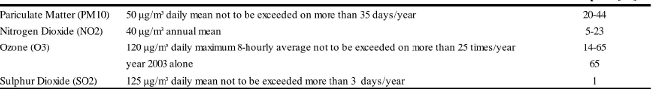
Tab. 1: Percentage of urban population exposed to air pollutants from 2001-2011 (Guerreiro, de Leeuw, & Foltescu 2013) ... 26 Tab. 2: Initial concentrations as used within the box model ... 38 Tab. 3: Urban parameter table for input to the urban parameterization scheme. Parameters are derived for the three CORINE based urban classes: commercial (33), high density (32) and low density residential (31). The lower part of the table is only valid for the BEP by representing the distribution of the buildings in height and street characteristics for each class (changed from Chen 2011) ... 54 Tab. 4: Sky View Factors calculated from building height H and road width W according to the formula of Oke (1982) ... 55 Tab. 5: Modelling setup used for meteorological part according to Skamarock et al. (2005) ... 58 Tab. 6: Most important parameters and schemes added to the modelling setup for WRF- Chem ... 63 Tab. 7: SNAP level 1 source categories 1 to 10 classified by the emission source ... 68 Tab. 8: Measurement stations used for evaluation of the urbanized WRF-Chem run ... 72 Tab. 9 Important meteorological features of urban and rural environments, presented as an average for the modelling period Aug 11 to Aug 17 2003 ... 84 Tab. 10 Atmospheric composition of urban and rural air, explained on the basis of selected primary and secondary compounds. Values represent mean urban and mean rural concentrations for the modelling period August 9 to August 17 2003 on a single urban and rural grid cell. The day (0700 h – 2200) is distinguished from the night (2300 h to 0600 h).
... 85 Tab. 11: Impact of urban planning strategies on mean and maximum urban temperature and UHI intensity calculated from model output for August 13 2003 8 pm. The control run indicates ‘real’ conditions. ... 95 Tab. 12: Effects of different urban planning scenarios on atmospheric characteristics within the urban canopy. Results are presented for the modelled mean at the urban grid cell as defined in Chapter 6.2. The same is displayed for a rural grid cell isolated from the area influenced by the city. The urban heat island is calculated from the difference between urban and rural mean temperature for both the surface (surface_UHI) and canopy UHI (2m_UHI). ... 98 Tab. 13: Effect of UHI mitigation scenarios on modelled runtime mean concentrations of O3, NO, NO2 and CO as well as formaldehyde (HCHO) and isoprene (C5H8) in the urban centre showing absolute values. In addition, the effect on mean potential 2m temperature is shown in the grey shaded area below. A decrease is presented in italics and the maximum effect is presented in bold. Normal formatting reveals an increase. ... 99 Tab. 14: Modelled relative effect on mean daytime and night-time concentration of NO, NO2, CO and ozone during Aug 09 - Aug 18 2003 ... 101
List of Tables
XXI Tab. 15: Difference in mean surface concentration between the north-west (NW) and south-east (SE) rural locations with regard to each scenario and control run ... 103 Tab. 16: Effects of the specific scenario on mean of turbulent kinetic energy (TKE) and planetary boundary layer height (PBLH) ... 105 Tab. 17: Components of the hourly budget as provided by WRF-Chem output for NO, NO2 and CO between 0800 and 0900 h (Unit ppbv h-1) with regard to the Control Run (Control) and the Albedo scenario. ... 112 Tab. 18: Components of hourly budget computed for O3 between 1600 and 1700 h (Unit ppbv n-1) ... 112
1. Introduction
1 1. Introduction
“As soon as I had escaped the heavy air of Rome and the stench of its smoky chimneys, which when stirred poured forth whatever pestilent vapours and soot they held enclosed, I felt a change in my disposition.” (Seneca, AD 61)
‘[…] in the denser parts of the metropolis, the heat is raised, by the effect of the population and fires […] and it must be proportionally affected in the suburban parts […]’ (Howard L. 1833: The Climate of London)
The roman philosopher Seneca (4 B.C. - 61 A.D.) stated the negative effect of urban air pollution for the inhabitants of the city of Rome during the age of the Roman Empire.
Luke Howard was the first to provide evidence that urban temperatures are elevated compared to the rural surroundings. Based on continuous measurements within the city of London and suburbs, he was the first to describe a phenomenon which was scientifically characterized as the Urban Heat Island (UHI) (Oke 1973) . With his concise statement of the temporal variation of urban-rural temperature differences and the analysis of spatial patterns, he laid the foundation for scientific research in the field of Urban Climate (Mills 2008). Since these times, a vast amount of studies have been performed, covering different fields (Solomon 2007), aspects and geographic regions. Urban climate has been explicitly treated in the recent IPCC Reports (AR4 and AR5) (Stocker et al. 2013).
We are living in a world of growing population and urbanization has become the key indicator of human development around the globe. Until 2050, the fraction of global urban population will increase to over 69% (Europe 82%), which means that about 6.3 billion people are expected to live in urban areas (United Nations 2012). Being the centres of human activity, urban areas are especially vulnerable to climate change and air pollution.
To maintain sustainable development and to cope with the growing population pressure, urban systems are reliant on a constant energy supply, which still is achieved mainly by burning of fossil fuels. Although covering less than 3 % of the land surface, cities are the main contributor to global greenhouse gas emissions. With 78 % of total global carbon emissions, they are heavily implicated in global climate change (Grimm et al. 2008). Urban agglomerations, which have grown rapidly over the last decades, now have to cope with a self-induced effect. If there is an impact of climate change on human beings, this impact will essentially affect urban environments (Stone Jr 2012).
1. Introduction
2
According to city size, building structures and population density, a city creates its own microclimate which can differ from the rural surrounding. The conventional structure of a city is characterized by its road networks, public transportation system and architectural properties. This requires natural open areas to be replaced by impervious sealed surfaces like concrete and asphalt. Surface sealing changes the hydrological properties of an area.
Runoff rates are increased and evaporation is reduced significantly. Next to this, urban materials tend to absorb the bulk of the incoming thermal radiation leading to the extensive accumulation of heat. The buildings act as obstacles for air circulation and heat can be trapped within street canyons where it can even remain hours after sunset. Additionally, anthropogenic heat amplifies the excessive warming of urban areas, which can in turn promote the formation of secondary circulation patterns between city and surroundings (Arnfield 2003). The annual mean temperature of central areas of a large city is about 1° to 3 °C higher than in the surrounding areas. In individual calm clear nights, it even can be up to 12 °C higher (Oke 1982a).
The UHI raises the demands of energy supply for air conditioning in summer periods. Air pollution correspondingly increases as connected with power plants and transportation relying on fossil fuels. According to the city structure and meteorological conditions, air pollutants can either remain within the city for long periods or be transported into the rural surrounding either by wind or via induced secondary circulation due to the urban-rural temperature gradient. Further, chemical reactions can be accelerated by the additional heat.
With increased urban growth and traffic volume, heat stress and worsened air quality have also developed into major problems in urban areas located in Europe. Older people and infants tend to suffer most from excessive heating. The European Heat Wave in the summer of 2003 developed into the single most catastrophic weather event to have haunted Europe since the beginning of weather observations. The EU estimated that more than 70,000 people within 12 countries died from heat related illnesses, more than ever recorded in a single event since WW2. Remarkably, Italy and France - two of the most developed and medically advanced societies in the world - alone witnessed over 40,000 deaths.
Because of France being one of the countries having suffered the most from the heat wave, this phenomenon often is referred to ‘La Canicule’ (Stone Jr 2012) .
In order to improve living conditions in future urban environments, adaptation and mitigation strategies discussed in scientific, and social, political and economic
1. Introduction
3 communities. Adaptation demands the adjustment of our habits and way of living to the changed climatic conditions. Mitigation implies the direct intervention into the system, to identify problems and to reduce negative aspects.
Several mitigation strategies have been discussed in the scientific community to reduce urban temperature and urban heat islands. White roofs and highly reflective façades tend to reflect incoming solar radiation, which in turn leads to a reduction of surface warming (Taha 1997b). The cooling of the building also reduces the amount of energy needed for air conditioning (Akbari et al. 1997). Planted roofs or generally vegetated surfaces transform sensible into latent heat via evaporation, leading to a net cooling. Another way to reduce urban temperatures is the modification of the building structure itself, which includes the orientation and specific characteristics of the building and road orientations to create fresh air corridors and facilitate air circulation.
Several numerical and experimental studies have been carried out in the past to confirm the positive effect of these strategies. Taha (1997b) discussed the impacts of surface albedo, evapotranspiration and anthropogenic heating. By analysing numerical simulations and measurements, he indicated that increasing vegetation cover can effectively reduce the surface and near surface temperature. By combining low altitude flight measurements and a mesoscale model, he demonstrated that increasing the albedo by 0.15 can reduce peak summertime temperatures for the urban area of Los Angeles by up to 1.5 °C. During the DESIREX Campaign 2008, Salamanca et al. (2012) simulated, that a higher albedo leads to a 5% reduction in energy consumption through air conditioning during summertime periods for the area of Madrid. Solecki et al. (2005) studied extensively the effect of urban vegetation in New Jersey by a GIS-based model application, while Zhou et al. (2010) numerically simulated the UHI of Atlanta under extreme heat conditions and stated that increasing the vegetation fraction and evapotranspiration are the most effective mitigation strategies for that area. The energy saving aspect of highly reflective surfaces is simulated on a more global perspective in Akbari et al. (2009) and Oleson et al. (2010), who treated white roofs in a global climate model as subgrid phenomena also accounting for air conditioning and heating demand. Jacobson et al. (2011) used a global model to analyse the effect of urban surfaces and white roofs on global and regional climate.
On the side of experimental studies, Onishi et al. (2010) evaluated the potential for UHI mitigation by greening parking lots in the city of Nagoya, Japan by analysing land surface
1. Introduction
4
temperature retrieved from a broad range of remote sensing datasets. The regional energy saving effect of high-albedo roofs can also be found in Akbari et al. (1997) who was running experimental measurements of microclimate and energy use at selected buildings.
It is well established that urban heat island mitigation strategies have an effect on dynamical processes in the urban canopy layer, whereas the effect on chemical reactions is not yet fully understood. The relation between the urban heat island and air quality is investigated in Lai and Cheng (2009) who showed that the concentration of pollutants increases with the UHI under certain prevailing weather conditions. Taha (1997a) pointed out that peak ozone concentrations at 3 p.m. can decrease by up to 7% with a massive increase of surface albedo, whereas Akbari et al. (2001) stated that urban trees and high- reflective roofs can significantly reduce energy consumption, thus improving air quality.
Analysing the effect of urban heat island mitigation strategies on urban air quality is the main focus of this dissertation. For this reason, the mesoscale numerical model WRF (Weather Research and Forecasting Model (Skamarock et al. 2005)) and the chemical model WRF-Chem (Grell et al. 2005) are used to analyse the urban climate and air quality on a regional scale. Different parameterization schemes are available in WRF to represent urban surfaces and dynamical processes in the urban atmosphere. (Chen et al. 2011a). A way of incorporating high resolution land use data is presented and the modification of an urban canopy model according to local urban properties is discussed. The first part deals with the effect of UHI mitigation strategies on local meteorology and dynamical processes by simulating different urban planning scenarios with regard to a medium sized European city (Stuttgart) during an extreme heat event. The basic results are presented in Fallmann et al. (2014). The second part discusses the effect of these strategies on the chemical composition of the urban air. Local observations from the city of Stuttgart are used to calibrate the model and evaluate the simulations.
The new contribution to the scientific field however will be the incorporation of high resolution land use data and the coupling of an urban canopy model to the chemical model WRF-Chem (Grell et al. 2005) for assessing the effect of certain urban planning scenarios on urban air quality on a regional scale. It is the first study of this kind to be performed for the urban area of Stuttgart and thus acts as test case for future simulations. Different studies have been carried out in the past, dealing with the effect of UHI mitigation strategies mainly on ozone concentrations (e.g. Akbari 2001). This study however extends
1. Introduction
5 the analysis towards secondary effects on primary pollutants such as carbon monoxide, nitrogen oxides and particulate matter coming along with a reduction of the urban temperature.
The study is funded by the EU-Project 3CE292P3 – ‘UHI - Development and application
of mitigation and adaptation strategies and measures for counteracting the global UHI phenomenon’. This project is implemented through the CENTRAL EUROPE Programme
co-financed by the ERDF. Within eight pilot areas, the project aims to develop strategies and policies for adaption and mitigation of the risks arising from urban heat island formation while being in close transnational discussion with policy makers, local stakeholders and professionals. The urban area of Stuttgart is one of the participating pilot regions and serves as test bed for executing model simulations.
Local processes and interactions like heat islands and urban air quality are driven by boundary conditions from larger scales. Hence, the understanding of small scale phenomena requires an explanation of the broader context in advance.
2. Global Background
6
2. Global Background 2.1 Climate Change
According to the IPCC Fifth Assessment Report AR5 ‘[…] each of the last three decades has been successively warmer than the preceding one. […] and human influence has been detected in warming of the atmosphere and the ocean […], and in changes in some climate extremes.[…] It is very likely, that the increased CO2 concentrations have led to a global warming trend in the last century[…]’ (Stocker et al. 2013).
The burning of oil, gas, coal and forests has been the driving force of industrial development since the middle of the 19th century. This created an imbalance in the carbon cycle so that the input into the system happens more rapidly than CO2 is being removed by assimilation processes in the ocean or terrestrial system. An additional anthropogenic greenhouse effect is generated which causes global temperatures to rise. The steady increase of atmospheric CO2 concentrations has been monitored at the Mauna Loa Observatory in Hawaii since the 1950s when 315 parts per million (ppm) was measured compared with 392 ppm in 2012 (Stone Jr 2012).
In order to project future climate conditions, scenarios of human activities and future socio-economic behaviour of the world population and economy have to be defined. In comparison with AR4 (Solomon 2007) in the Fifth Assessment Report (AR5), the scientific community has developed new ways to characterize future developments by defining four new scenarios following the theory of Representative Concentration Pathways (RCP) (Moss et al. 2010). Each pathway is identified by its approximate radiative forcing in the year 2100 relative to 1750 and represents a range of 21st century climate policies resulting in different intensities of greenhouse gas emissions. Radiative forcing describes the net irradiance at the top of the atmosphere (TOA) calculated from downward minus upward fractions and is modified by the change in concentrations of chemical constituents like carbon dioxide (Stocker et al. 2013)
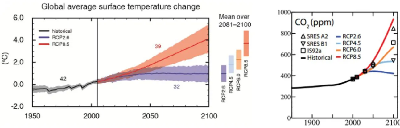
Following the outcome of IPCC AR5, global surface temperature change for the end of the 21st century is likely to rise by 1.5 - 4 °C relative to the period 1850-1900 for all scenarios.
With regard to global mean sea level rise, the range of values reaches from 0.24 to 0.3 cm and from 0.4 to 0.63 cm, respectively. The global CO2 level is supposed to rise from about 300 ppm historically to over 900 ppm at most in 2100 (Fig. 1) (Stocker et al. 2013).
2. Global Background
7
Fig. 1: Projected temperature (left) and CO2 (right) increase for each RCP Scenario (Stocker et al. 2013)
Due to elevated temperatures, secondary effects will be generated and amplified which will in turn also affect urban environments. The number of summer precipitation events is supposed to decrease, whereas winter months will register an increase. Heavy thunderstorms and very heavy precipitation events will occur more often in the future. An increased frequency of thermal extremes as well as an increase in duration, frequency and intensity of heat waves is very likely. Next to the rising temperature itself, elevated concentrations of air pollutants can become harmful to human health (Kuttler 2012;
Solomon 2007). How extreme events affect societies was dramatically proven by the European Heat Wave 2003. Around 2002 heat-related deaths were recorded on a single day in August alone in France, 600 in Spain and another 250 in four Italian cities. Nearly 650,000 ha of land had been destroyed by fires by the end of summer 2003 and the impact on harvest and livestock was dramatic. Massive drought has led to water scarcity where falling river levels affected important European trade routes. The financial loss resulting from the heat wave is estimated to be about $13 billion, which is maybe still underestimating the true costs. Not only the human body, but also urban infrastructure can suffer from long periods with elevated heat stress which can result in distortions of construction materials of buildings or public transportation and derogate electrical power supply (Stone Jr 2012). Urban environments will suffer from climate change and moreover, the risks are amplified by human activities.
2. Global Background
8
2.2 Population growth and urbanization
Next to rising temperatures, the planet has to face a constantly increasing pressure of the global population on land and resources. Since the beginning of the 19th century, the number of people living on Earth has grown from one to over seven billion today and is expected to increase by another 2.3 billion till 2050. Additionally, urbanization demands the transformation of natural landscape to sealed areas leading to a loss of huge amounts of biosphere.
From 1950 till 2010, the percentage of people residing in cities has increased from 30 % to 52 % and is projected to exceed 67 % by 2050. Less developed countries will have to face especially dramatic problems when the standard of development cannot keep pace with the demands of the fast growing population. The number of megacities with at least 10 million inhabitants will increase. With Tokyo (23.3 million) and New York (16.2 million) in the year 1970, only two megacities existed. This number increased to 10 in 1990, up to 23 in 2011 and is expected to rise to 37 in 2025. At present with 37.2 million people, Tokyo is ranked first globally. The three countries with the largest increase in urban population between 2000 and 2050 will be India, followed by China and Nigeria (United Nations 2012).
Between 1970 and 2011, the number of people living in megacities has grown from 39.5 to 359.4 million and is expected to almost double to 630 million by 2025, meaning one in 13 people will be living in a megacity. These huge urban agglomerations are dynamical systems which react to the projected climate change in all its facets (United Nations 2012) Although urban areas only cover a small fraction of the land surface, it is assumed that they contribute to climate change. According to Kalnay et al. (2003), the impact of urbanization on temperature trends in the continental United States accounts for 0.06 and 0.15 °C per century, depending on the method; one is based on population data, the other on satellite measurements of night light.
Based on the United Nations World Urbanization Prospects 2011 Revision Report (United Nations 2012), in 2011 60 % or about 890 million people were living in areas with a high risk of being affected by natural hazards. Flooding is seen as the most frequent and intense hazard when climate change amplifies the frequency of extreme weather events and the sea
2. Global Background
9 level rises due to global warming. Droughts, which can evoke heat waves, are ranked in second place.
The vulnerability of urban population to climate change is not only related to the growing number itself, but also to an over-aging of the population which happens particularly in OECD countries. By 2050, about 25 % of the people are projected to be older than 65 compared to 15 % today. This massive aging of the population will bring a range of new problems to urban areas regarding the health sector, especially in periods of extreme weather events or heavy air pollution (United Nations 2012).
2.3 Energy consumption and air quality
Cities are dynamic systems which have to constantly satisfy the needs of their inhabitants concerning residential, transportation and economic sectors. Each sector claims a huge demand of energy. With an annual average growth rate of the Gross Domestic Productivity (GDP) of 3.6 %, the global need for energy consumption is expected to increase dramatically within the next 50 years (OECD 2012).
In 2010, the building sector (excluding industrial facilities) consumed more than 20 % of the global delivered energy. Due to the rapid growth of urban systems along with changes in living standards and economic conditions, the energy growth in the building sector is the fastest throughout all projections of the International Energy Agency (IEA). The total global energy demand for buildings shows an annual growth rate of 1.6 percent per year.
Although in OECD countries this increase is less intense, in fast growing non-OECD countries this number can rise up to 2.7 %, accounting for nearly 80 percent of the growth in the world’s total building sector energy consumption (Birol 2013).
About 85 % of the world’s energy is still supplied by fossil fuels like oil, gas and coal.
Resources are exploited and renewable energy still does not have the efficiency to fill the gap when the economically viable energy from oil and gas reserves are depleted (Visser et al. 2009).
According to projections of the OECD – Transport Outlook 2011, an increasing level of globalization will lead passenger mobility to triple by 2050. Expecting the global number of cars to rise from 700 million (2011) to nearly 2 billion in 2050, CO2 emissions from
3. The Urban Climate
10
vehicle use are also assumed to triple despite new technologies for fuel and emission reduction can be effectively used (OECD 2011). In the European Union, CO2 emissions from road transport are responsible for approximately one fifth of the EU's total emissions.
Between 1990 and 2010, they have increased by 23 % (Guerreiro et al. 2013).
Nitrogen oxides, volatile organic compounds (VOC) which result from incomplete combustion of fuel and photochemical oxidants like ozone are mainly connected to increased traffic in the urbanized world (Fenger 1999). For cities acting as sources of emissions, ambient concentrations can have widespread effects on human health, urban and regional visibility, ecosystem degradation and on a broader scale, regional climate change and global pollutant transport. (Molina and Molina 2004)
When mobility and social standards are increasing, urban dwellers expand their activities well beyond the city borders, leading to an increase in the ecological footprint and resulting in a constantly increasing pressure on the surrounding ecosystem (Grimm et al.
2008).
3. The Urban Climate 3.1 Introduction
Urban climates significantly differ from those of rural areas, depending on prevailing weather conditions, building geometry and material, anthropogenic heat sources and thermo-physical characteristics (Taha 1997b). Urban climatology as defined in Oke (1987) addresses the mass, momentum and energy transfer through an urban area and entails modified physical variables like temperature, humidity or wind speed which alter circulation patterns, chemical reactions and transport of pollutants.
The analysis of a vast amount of observational data reveals that urban areas in the northern hemisphere annually have an average of 12 % less solar radiation, 8 % more clouds, 14 % more rainfall, 10 % more snowfall and 15 % more thunderstorms compared with the rural surrounding. Urban temperatures can be on average 2 °C higher and the concentration of air pollutants can exceed those of an ‘undisturbed’ atmosphere by 10 times.
Evapotranspiration rates from sealed surfaces can be decreased by up to 60% and summertime humidity by 20%. Obviously, fluxes of heat, moisture and momentum are
3. The Urban Climate
11 modified by the urban canopy and are even further enhanced by human activities (Taha 1997b).
The feedback of global processes to the regional and urban scale is closely coupled to the city’s orientation, shape and complex morphology. Due to a high degree of heterogeneity, urban areas offer a great diversity of surfaces and a broad range of spatial scales, which leads to diverse effects in the energy balance. The physical mechanisms responsible for the modification of the regional and local climate occur and interact on different scales both in time and spatial dimensions (Britter and Hanna 2003).
Fig. 2: Interactions across scales in atmospheric modelling (Britter & Hanna 2003)
The time scales range from one second and below for turbulent motions, over hours for the formation of convective cells which produce cumulus clouds, to seasonal or yearly time scales.
Urban-rural interactions and circulation patterns influenced by the urban heat island occur from meso to sub-meso or regional scales and directly affect the regional climate by modifying weather patterns. Urban air pollution and the effect of increased heat on human health reach from the neighbourhood down to the street scale with processes differing between street canyons. A heat island itself can occur on different scales; around a single building, city quarter or the whole urban canopy.
3. The Urban Climate
12
The elevated urban temperatures for urban dwellers may be beneficial in winter periods due to a decreased heating load as well as a reduced snow or ice loading on urban roads.
However, the negative aspects concerning heat stress such as an increased energy consumption for cooling and a diminished air quality are dominating factors (Taha 1997b).
Temperature as perceived by human beings depends on a number of factors. Next to the measured temperature itself, factors like moisture, exposure, physiological conditions, clothing and behaviour define the physiological equivalent temperature (PET) which serves as an indicator for the well-being of urban dwellers and characterizes a key parameter in the research field of biometeorology (Höppe and Hurk 1999).
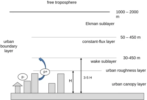
Atmospheric characteristics mirror distinct features of the urban canopy underneath, which leads to the formation of characteristic layers (Fig. 5). According to Oke (1987), the urban atmosphere can be divided into an urban canopy layer (UCL) and an urban boundary layer (UBL), although the transitions can be poorly defined. The UCL which also includes the skin of the urban surface extends from the ground up to the mean roof level and is dominated by absorption and reflection processes within the urban canopy. Per definition it is part of the planetary boundary layer (PBL). The PBL or mixing layer refers to the air volume near the ground that is directly affected by diurnal heat, moisture or momentum transfer to or from the surface. Within this compartment of air, turbulent motion is high and vertical mixing is strong. The top of the boundary layer is characterized by a temperature inversion, a change in air mass, a rapid change in moisture and wind speed and/or wind direction.
Heat propagating through the building material and the ground surface can be accumulated in deeper layers beneath the surface which can lead to warming there. Interactions and processes in the urban atmosphere induced by the presence of a city are expressed as mesoscale for urban-rural interaction, to a local scale for city quarter interaction, down to micro scale processes within urban canyons.
3. The Urban Climate
13
Fig. 3: Urban environments in atmospheric processes across a range of scales (Oke 1987)
In Section 3.2, the Urban Heat Island is defined based upon its physical nature, energetic basis, attached problems and risks related to heat and air quality. Moreover, mitigation strategies are defined and discussed in Section 3.3.
3.2 Urban heat island characteristics
The atmospheric state is a response to the exchange of sensible and latent heat and mass and momentum. In urban areas, the sources and sinks for these exchanges originate from interactions in a heterogeneous environment, involving natural as well as anthropogenic factors. The urban heat island is a regional climate phenomenon induced by the radiative properties of impervious surfaces, leading to aggravated heat accumulation and a positive temperature difference between the urban area and rural surroundings. The urban heat island can be clearly distinguished by analysing the surface temperatures of an urban surface in comparison with the rural surroundings. Isotherms for near surface air temperatures reveal a sharp border between the urban and rural environment which leads to the analogy of an ‘island’ (Fig. 4).
3. The Urban Climate
14
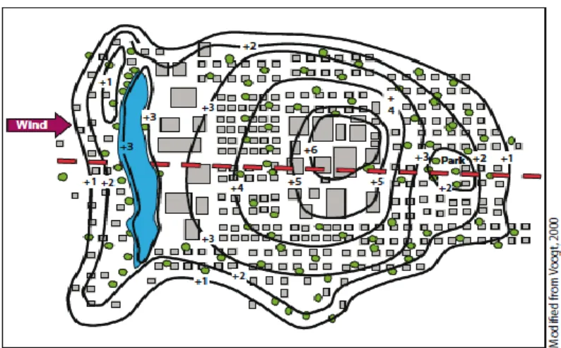
Fig. 4: Contour lines of equal UHI Intensity (EPA 2013)
The horizontal temperature gradient throughout the urban area reflects the city structure while revealing areas of higher building density, whereas single urban parks or lakes might lead to detached cool spots (Voogt and Oke 2003). However, the shape and the characteristics of the UHI are strongly connected to the diurnal cycle of incoming shortwave radiation. Due to rapid night-time cooling of the rural surrounding and the high heat storage capacity of impervious surfaces, the difference in near surface air temperature is highest during the evening and night. Hence, the UHI is mostly pronounced at night and in the periods around sunset and sunrise. In urban areas, warming and cooling rates are generally smaller which leads to a damping of the diurnal temperature curve. Urban areas are characterized by low wind speeds that are especially pronounced when fresh air corridors are blocked by buildings or naturally by morphological features that hinder air mixing and cooling while further promoting the heating of surfaces and temperatures.
Next to the geographical location of a city, topographic features, the nature of soils, vegetation and land use, there is an evident relation between the heat island intensity and the city size or population density.
With population density (P) being an indicator for the size of a city, Oke (1973) found a logarithmic relationship between city size and the UHI intensity. Analyzing the maximum heat island (given as ∆Tu-r(max)) for 11 European cities with more than 50,000 inhabitants, he identified a simple formula:
∆𝑇𝑢−𝑟(𝑚𝑎𝑥)= 2.01 𝑙𝑜𝑔10𝑃 − 4.06. (3.1)