Trimmed likelihood estimators for stochastic differential equations with an application to crack growth analysis from photos

SFB 823

for stochastic differential

equations with an application to crack growth analysis from photos

Discussion Paper Christine H. Müller, Stefan H. Meinke

Nr. 70/2016

differential equations with an application to crack growth analysis from photos

Christine H. Müller and Stefan H. Meinke

Abstract We introduce trimmed likelihood estimators for processes given by a stochastic differential equation for which a transition density is known or can be approximated and present an algorithm to calculate them. To measure the fit of the observations to a given stochastic process, two performance measures based on the trimmed likelihood estimator are proposed. The approach is ap- plied to crack growth data which are obtained from a series of photos by back- tracking large cracks which were detected in the last photo. Such crack growth data are contaminated by several outliers caused by errors in the automatic image analysis. We show that trimming 20% of the data of a growth curve leads to good results when 100 obtained crack growth curves are fitted with the Ornstein-Uhlenbeck process and the Cox-Ingersoll-Ross processes while the fit of the Geometric Brownian Motion is significantly worse. The method is sensitive in the sense that crack curves obtained under different stress con- ditions provide significantly different parameter estimates.

Christine H. Müller

Department of Statistics, TU Dortmund University, D-44227 Dortmund, Germany cmueller@statistik.tu-dortmund.de

Stefan H. Meinke

Department of Statistics, TU Dortmund University, D-44227 Dortmund, Germany stefan.meinke@uni-dortmund.de

1 Introduction

The motivation of this paper is the analysis of micro crack growth data obtained from photos of the surface of a steel specimen exposed to cyclic load. A simple model for crack growth is given by the Paris-Erdogan equation (see e.g. Pook, 2000)

d a

d N = C (∆ σ √

a)

, (1)

where a is the crack length, N the number of load cycles, C and m are usu- ally unknown constants and ∆ σ = σ

− σ

is the range of the cyclic stress amplitude. Since crack growth is not a deterministic process, several stochas- tic versions of the Paris-Erdogan equation were developed (see e.g. Ortiz and Kiremidjian, 1988; Ray and Tangirala, 1996; Nicholson et al, 2000; Wu and Ni, 2004; Chiquet et al, 2009; Hermann et al, 2016a,b). Often only models are developed but no statistical analysis is presented. For example, the books of Sobczyk and Spencer (1992), Castillo and Fernández-Canteli (2009), Sánchez- Silva and Klutke (2016) are full of models but besides some simple statistical methods not much is provided.

One approach is to extend equation (1) with an additive stochastic term lead- ing to a stochastic differential equation (SDE), see e.g. Lin and Yang (1983), Sobczyk and Spencer (1992), Wu and Ni (2004), Zárate et al (2012), Hermann et al (2016a,b). The advantage of a SDE is that several statistical methods were developed already, at least for some of them, see e.g. Sørensen (2004) or Iacus (2008). In particular likelihood methods were proposed as in Pedersen (1995), Beskos et al (2006), Pastorello and Rossi (2010), Sun et al (2015), Höök and Lindström (2016). However, the choice of the SDE is still a problem. More- over, usually the crack growth data are not so nice and numerous as those of Virkler et al (1979), who provided 68 series with 164 measurements in a labo- rious study. These measurements are nice since they do not include many big jumps and errors in contrast to other crack growth data as those considered in Kustosz and Müller (2014) and Hermann et al (2016a) where additionally less than ten series were observed.

With automatic detection of crack growth from photos it is possible to obtain

a much larger number of series of crack growth data and it is much less labo-

rious. The resulting large data sets allow a better analysis of the crack growth

and the corresponding fatigue behavior of the material. However, those data

contain several errors originated by the automatic detection. These errors are

for example caused by scratches and contaminations of the material, blurred photos, shadows on the photos and other image processing problems and pro- vide outliers in the crack growth curves. In particular they can cause that the growth curve is not strictly increasing.

To cope with such outliers, we propose to use trimmed likelihood estima- tors for SDEs. Trimmed likelihood estimators for independent observations were introduced by Hadi and Luceño (1997). They extend the least median of squares estimators and the least trimmed squares estimators of Rousseeuw (1984) and Rousseeuw and Leroy (1987) by replacing the likelihood functions of the normal distribution by likelihood functions of other distributions. Müller and Neykov (2003) applied them for generalized linear models and other ap- plications can be found for example in Neykov et al (2007), Cheng and Biswas (2008), Neykov et al (2014), Müller et al (2016). Because of the trimming of a proportion of the data, trimmed likelihood estimators can deal with a amount of outliers up to the trimming proportion. We use trimmed likelihood estimators here to define two measures for the performance of a fit of a SDE to the data.

One performance measure is based on the median of absolute deviations of predictions and the other is based on the coverage rate of prediction intervals.

The paper is organized as follows. In Section 2, the trimmed likelihood es- timator together with its computation is introduced and the two performance measures based on the trimmed likelihood estimator are proposed. Section 3 provides the application to crack growth data obtained from photos. Therefore, at first, it is described how crack growth curves can be obtained by backtrack- ing long cracks which were detected in the last photo in a series of photos.

Then the fits of three SDEs to these curves are obtained with trimmed like-

lihood estimators with different trimming rates and are compared via the two

performance measures. Moreover, the fits of curves from two experiments with

different stress conditions lead to significantly different parameter estimates

so that the approach can be used to distinguish between different stress condi-

tions. Finally, Section 4 discusses the results and some further extensions.

2 Trimmed likelihood estimators for SDEs

2.1 Trimmed likelihood estimators and their computation

A stochastic extension of the Paris-Erdogan equation (1) is given by the stochastic differential equation

dX

= b(X

,θ) + s(X

,θ )dB

where the time-continuous stochastic process (X

)

provides the crack size, b and s are known functions, (B

)

is the standard Brownian Motion, and θ is an unknown parameter vector. Special cases are given by

dX

= (θ

+ θ

X

)dt + θ

X

dB

,

with θ = (θ

, θ

,θ

,γ)

⊂ R

which include the Ornstein-Uhlenbeck process (γ = 0), the Cox-Ingersoll-Ross process (γ = 0.5), and the Geometric Brown- ian Motion (θ

= 0, γ = 1), see e.g. Iacus (2008). The process is observed at time points 0 ≤ t

< t

< . . . < t

providing observations x

, ..., x

.

The idea of trimming is to use only a subset I = {n(1), . . . , n(I)} of {0, 1, . . . , N} with 0 ≤ n(1) < n(2) < . . . < n(I) ≤ N. Since the conditional dis- tribution of X

given X

is often known or at least can be approximated, we set

p

(x

|x

n(i)

)

for the transition density of the conditional distribution or its approximation.

Then the likelihood function for the observation vector x

:= (x

, ..., x

) is given by

l

(x

) =

I−1

∏

i=1

p

(x

|x

).

If I = {0,1, . . . , N} then the classical maximum likelihood estimator is given by

θ b := arg max

θ

l

(x

).

We can also define the maximum likelihood for any subset I ⊂ {0,1, . . . , N}

as

θ b ( I ) := arg max

θ

l

(x

)

so that θ b ( I ) = θ b if I = {0,1, . . . , N}. A H-trimmed likelihood estimator is then defined as (see e.g. Hadi and Luceño, 1997; Müller and Neykov, 2003)

θ b

:= θ( b I

) with I

∈ arg max{l

θb(I)

(x

); I ∈ J

},

where J

:= { I ⊂ { 0,1, . . . , N} ; ] I = N − H +1 } and ]A denotes the num- ber of elements of a set A. In the H-trimmed likelihood estimator, the H most unlikely observations are trimmed, i.e. not used. If H = 0, i.e. no observation is trimmed, then we get again the maximum likelihood estimator so that θ b

= θ. b

●

●

●

●

●

●

●

1 2 3

●

●

●

●

●

●

●

● i−1 i i+1 i+2

●

●

●

●

●

●

●

I−2 I−1 I

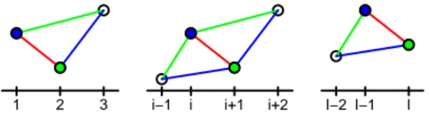
Fig. 1 Remaining transition densities if the observation att_n(i)(blue) or att_n(i+1)(green) is trimmed because the transition densityp_i+1|i(red) is small, for the casei=1 (on the left),i∈ {2, . . . ,I−2}

(in the middle),i=I−1 (on the right)

If N is small or H is very small then the H-trimmed likelihood estimator can be calculated by considering all subsets I ∈ J

. If this is too time consuming then approximate algorithms based on a genetic algorithm and a concentration step as proposed in Neykov and Müller (2003) or based on a special selective iteration as proposed in Rousseeuw and Driessen (2006) can be used. However the concentration step is here much more complicated as in the case of inde- pendent observations since a single transition density p

:= p

(x

|x

) is influenced by two observations, see Figure 1. Hence if p

(x

|x

) is small it is not clear whether x

or x

should be trimmed. Hence we pro- pose the following procedure as concentration step.

As in the independent case, the concentration step starts with an initial sub- set I

with N −H +1 elements and provides a new subset I

with N − H + 1 elements. Set for simplicity θ = θ( b I

) and define the transition densities

p

:= p

( I ) := p

(x

|x

) for j > i and p

:= p

for any set I = {n(1), . . . , n(I )} with 0 ≤ n(1) < n(2) < . . . < n(I) ≤ N. The

idea is now to start with the complete sample, i.e. I (0) = { 0,1, . . . , N} , where

no observation is trimmed. Then observations one after another are removed until a set I

with N −H + 1 elements is obtained. For that, only the transition densities p

depending on θ = θ( b I

) are used.

Algorithm for the concentration step

1) Initialize I (0) = { 0,1, . . . , N} and I(0) = N + 1.

2) For h = 0,1, . . . , H − 1 do:

3) Set I = I (h), I = I(h).

4) Determine the ordered transition densities inside I , i.e.

p

≥ p

≥ . . . ≥ p

with {π (1), π(2), . . . , π(I − 1)} = {1,2, . . . ,I − 1}.

5) If π(I − 1) = 1 then (see left figure in Figure 1):

if p

≤ p

then I (h + 1) = I \ {n(1)}

else I (h + 1) = I \ {n(2)}.

6) If π(I − 1) = I − 1 then (see right figure in Figure 1):

if p

≤ p

then I (h + 1) = I \ {n(I − 1)}

else I (h + 1) = I \ {n(I)}.

7) If i := π(I − 1) ∈ {2, . . . , I − 2} then (see middle figure in Figure 1):

if p

· p

≤ p

· p

then I (h + 1) = I \ {n(i)}

else I (h + 1) = I \ {n(i + 1)} . 8) h ← h + 1 and I(h) ← I −1.

9) If l

θ(bI(H))

(x

) > l

θ(bI0)

(x

) then I

= I (H) else I

= I

. Step 9) is necessary since l

θb(I(H))

(x

) < l

θb(I0)

(x

) could happen so that I (H) is worse than I

. This is in opposite to the concentration step for in- dependent observations where the resulting trimmed likelihood is never worse then the starting trimmed likelihood.

Then a genetic algorithm for the optimization is proposed as follows.

Genetic algorithm

1) Start with M sets I

, . . . , I

∈ J

.

2) Concentration: Calculate I

, . . . , I

with the concentration procedure and replace I

, . . . , I

by I

, . . . ,I

, i.e. I

← I

, m = 1, . . . , M.

3) Mutation: Exchange in each set I

, . . . , I

∈ J

randomly k elements to

get further sets I

, . . . , I

∈ J

.

4) Recombination: Choose randomly N − H + 1 elements of the unions I

∪ I

, m = 1, . . . , M, to get further sets I

, . . . , I

∈ J

.

5) Selection: Determine from I

, . . . , I

the M sets with largest l

θb(I)

(x

).

Rename them as I

, . . . , I

. 6) Repeat Steps 2) to 5) until l

θ(bI)

(x

) is not improved anymore or a given number of repetitions is reached.

2.2 Performance measures based on trimmed likelihood estimators To define performance measures for the goodness-of-fit of the models esti- mated with the H-trimmed likelihood estimator θ b

, let be I

= {n(1), . . . , n(N − H + 1)} ∈ arg max{l

θ(bI)

(x

); I ∈ J

}. If the transition density

p

(x

|x

) is known or is given as approximation then the conditional ex-

pectation E

(X

|X

= x

) and the conditional quantiles l

(θ ) := F

α 2

X

= x

, u

(θ) := F

1 − α 2

X

= x

with F

(x) := P

X

≤ x|X

= x

can be determined.

The first performance measure is the median absolute deviation (MedAD) defined as

MedAD := median

|x

− E

θbH

(X

|X

= x

)|

∆

, . . . ,

|x

− E

θbH

(X

|X

= x

)|

∆

! . The absolute deviations are divided by ∆

:= t

−t

to take into account the different time differences t

− t

between the used observations.

The second performance measure is given by the (1 − α )-prediction inter- vals for X

based on the former observations x

for i = 1, . . . , N − H. If θ is known then a (1 − α)-prediction interval for X

is [l

(θ ),u

(θ )], i.e.

P

(X

∈ [l

(θ ),u

(θ )]|X

= x

) ≥ 1 −α is satisfied. If θ is unknown

then an estimate for θ can be used. Here we use the H-trimmed likelihood es-

timator θ b

as plug-in estimate. As performance measure, the mean length or

the coverage rate of the prediction intervals could be used. But it is better to use a combination of both. Hence the second performance measure is defined by

IS

:= 1 N − H

N−H

∑

i=1

S

(l

( θ b

), u

( θ b

);x

)

∆

where S

(l,u; x) := (u − l) +

(l − x)1

+

(x − u)1

is the interval score of Gneiting and Raftery (2007) for prediction or confidence intervals.

Thereby 1

denotes the indicator function. For prediction, as used here, the interval score S

(l,u; x) combines the length u − l of the prediction interval [l,u] with a penalty depending on α for the case that the predicted value x is not lying in [l,u]. Since larger time differences t

− t

lead to larger prediction intervals and smaller coverage rates and thus larger interval scores, we again divide the interval scores by ∆

.

Remark 1. For example, the conditional distribution of X

given X

is a normal distribution with mean

x

+

2

e

−

2

and variance

θ₃²(e^2θ2tn(i+1)−1)

2θ2

for the Ornstein-Uhlenbeck process, a log-normal distribution with mean x

e

and variance x

n(i)

e

(e

− 1) for the Geomet- ric Brownian Motion, and non-central χ

distribution with mean

x

+

2

e

−

θ2

and variance x

θ2

+

θ2tn(i+1))² 2θ₂²

for the Cox-Ingersoll-Ross process (see e.g. Iacus, 2008).

Remark 2. If the conditional distributions of X

given X

are not known, then approximations of the SDE can be used. The Euler-Maruyama approxi- mation provides for example (see e.g. Iacus, 2008)

X

− X

≈ b(X

,θ ) ∆

+ s(X

, θ) p

∆

E

where E

has a standard normal distribution so that p

(x

|x

) ≈ p

i,σ_i²)

, where µ

:= x

+ b(x

, θ) ∆

, σ

:= s(x

,θ ) √

∆

, and p

is the den-

sity of the normal distribution with expectation µ and variance σ

. In par-

ticular, we have E

(X

|X

= x

) ≈ x

+ b(x

, θ) ∆

. Hence the H-

trimmed likelihood estimator can be calculated via the densities of the approx-

imated normal distributions and the performance measures can be based on the

expectations and quantiles of the approximated normal distributions.

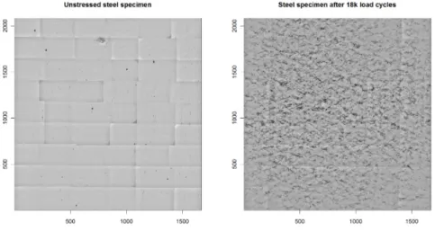
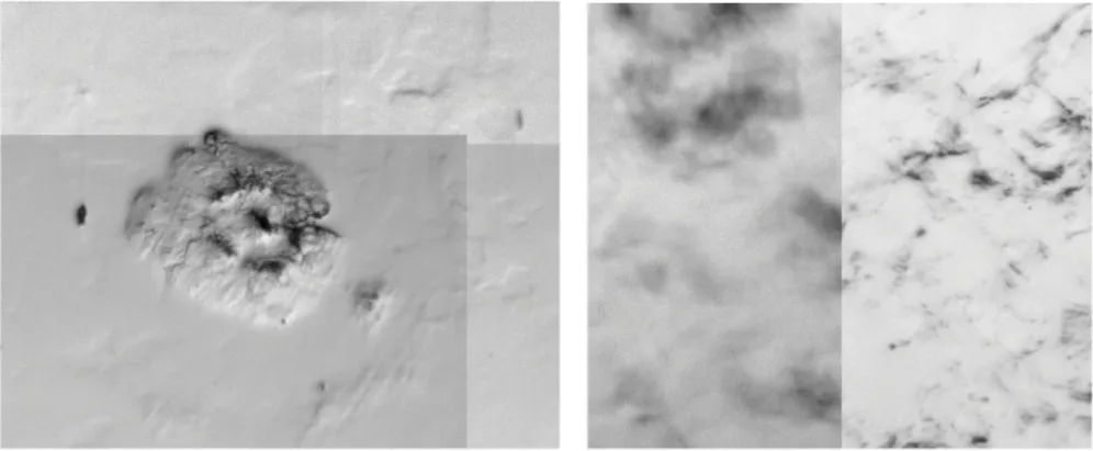
Fig. 2 Surface of an unstressed steel specimen (left) and after 18 000 load cycles (right) of a tension- compression-experiments with an external stress of 400 MPa

3 Application to crack growth data from photos 3.1 Obtaining crack growth data from photos

Figure 2 shows two photos of the surface of a steel specimen (Specimen 31), one before the specimen was exposed to cyclic load and one after 18 000 load cycles. During the 18 000 load cycles, a large number of micro cracks has ap- peared, visible by lower (blacker) pixel values. There exist several other photos at other time points, in this case for example after 1 000, 2 000, 3 000, 4 000, 5 000, 6 000, 7 000, 8 000, 9 000, 10 000, 12 000, 14 000, 16 000 load cycles.

For more details of the photos and the underlying experiment, see Müller et al (2011).

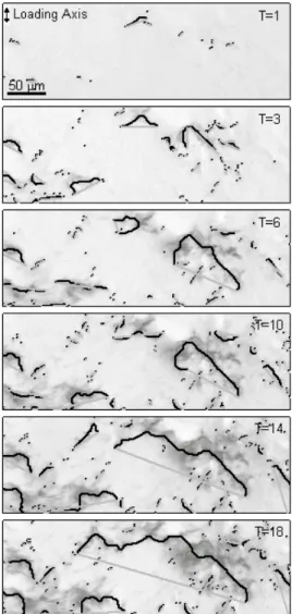
The first step is to detect the micro cracks in each of these photos by an existing crack detection algorithm as given for example by Purcell (1983), Cheu (1984), Buckley and Yang (1997), Fletcher et al (2003), Iyer and Sinha (2005), Fujita et al (2006), Yamaguchi and Hashimoto (2010), Gunkel et al (2012), Wilcox et al (2016). Figure 3 shows the detected cracks after 1 000, 3 000, 6 000, 10 000, 14 000, 18 000 load cycles in a cutout of the images.

These cracks were detected by the crack detection algorithm of the package

Fig. 3 Detected cracks in a cutout of the image after 1 000, 3 000, 6 000, 10 000, 14 000, 18 000 load cycles where T stands for the time in 1 000 load cycles

crackrec of Gunkel et al (2012), which is an R package (R Core Team,

2015) and free available at Müller (2016). This algorithm determines at first

so called crack clusters as connected sets of pixel positions below a threshold

value. Then a so called crack path in a crack cluster is the longest path which

can be found by Dijkstra’s shortest path algorithm connecting arbitrary pixel

positions of the crack cluster. These paths are marked in black in Figure 3.

The start and the end point of a crack path are connected by a straight line to highlight the crack paths. Figure 3 shows clearly how the number of detected cracks increases and how existing cracks becomes longer when the number of load cycles increases. Thereby, cracks can become longer also by the fusion of two or more cracks. Similar results will be obtained by other crack detection tools. For example UTHSCSA Image Tool of Wilcox et al (2016) provides also crack clusters but describe the orientation of cracks only by ellipses and rectangles. Crack paths are not detected.

The second step is to backtrack large cracks which were detected at the end. Large cracks could mean large crack clusters or long crack paths if paths are detected. However, since all crack paths are surrounded by crack clusters and paths are thin, the backtracking is based on crack clusters. Hence this step can be performed also by crack detection methods which provide only crack clusters.

The backtracking step is iterative. Assume that there are time points t

<

t

< . . . < t

for which detected cracks exist. For any chosen crack at time t

with 1 ≤ n ≤ N, all detected crack clusters at time t

are calculated which intersect with the chosen crack cluster. Then the largest crack is chosen as the predecessor of the chosen crack and becomes the starting crack for the next iteration. Thereby largest crack can mean a cluster with largest number of pixels or a cluster with longest detected path in the cluster. The K largest cracks at the last time point t

are used as starting cracks.

If, for example, cracks are determined by crackrec of Gunkel et al (2012) then the K

detected crack clusters C

(1), . . .C

(K

) of an image at time t

are given as a list called crackclusters which includes K

matrices M

(k) ∈ ℜ

of the corresponding pixel positions for k = 1, . . . , K

. Moreover, the list element cracks is a 6 × K

matrix which provides, for each of the K

clusters, the number n

(k) of pixels in the cluster, the length of the detected crack path in the cluster and the start and end points of the detected crack path.

Hence easily the largest cracks can be determined independently whether the size is measured in number of pixels of the cluster or the length of the crack path. Assume that C

(1), . . .C

(K) are the K largest clusters at the last time point t

. Then the proposed algorithm is as follows.

Backtracking algorithm 1) For k

∈ {1, . . . ,K}:

2) For n from N to 1:

3) If n = N set k = k

.

4) For any column c

(k) ∈ ℜ

of M

(k):

For j = 1, . . . , K

:

If the first component of c

(k) is contained in the first row of M

( j), i.e. the first component of c

(k) is contained in the first components of members of cluster C

( j) at time t

, then cre- ate a submatrix of M

( j) for which the first row is identical with the first component of c

(k).

If the second component of c

(k) is contained in the second row of this submatrix, then the intersection of C

(k) and C

( j) is not empty. Hence C

( j) is a candidate for the predecessor of C

(k) and j is stored in the list of predecessor candidates of k.

5) If the list of predecessor candidates is empty then set n = 0 so that the algorithm stops.

Else determine j as the largest crack within the predecessor candi- dates, set k = j, and reduce n by 1.

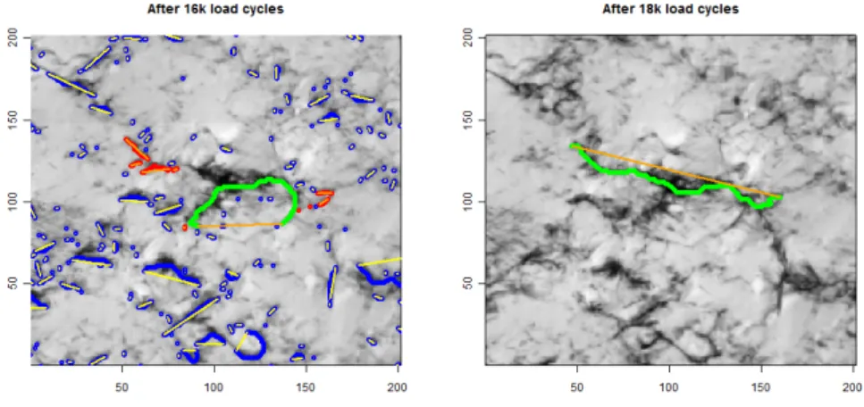
Fig. 4 Right: chosen crack in green after 18 000 load cycles, left: all detected cracks paths after 16 000 load cycles in blue, red, green, all predecessor cracks of the crack on the right in red and green, and the largest predecessor in green.

The iteration is demonstrated in Figure 4. On the right-hand side of this

figure, the chosen crack k at a time point after 18 000 load cycles is given in

green by its crack path. It is seen that the surrounding black area do not follow

completely the path so that the corresponding crack cluster is must larger. The left-hand side of the Figure 4 provides the detected crack paths after 16 000 load cycles which is the predecessor time point with an available photo. All detected crack paths are marked in blue, red, and green. All paths of the prede- cessor candidates, i.e. of crack clusters which intersect with the chosen crack cluster on the right-hand side, are marked in red and green. Clearly the green one is the longest predecessor so that it is chosen as predecessor crack and provides the new k for the next iteration. Its crack path is quite different from the green crack on the right-hand side since the crack cluster on the right-hand side is not given around one line. But it is the predecessor crack in any case, using the number of pixels in the cluster as well as the path length as crack size.

●

● ● ● ● ●

● ● ● ● ●

●

●

●

0 5000 10000 15000

050100150

load cycles

crack length

● ●

●

●

●

●

●

● ●

●

●

● ●

0 5000 10000 15000

050100150

load cycles

crack length

Fig. 5 Two resulting crack growth curves

For getting crack growth curves, one can use the number of pixels of the crack cluster as well as the length of the crack path in the cluster indepen- dently how the predecessor crack was obtained. Figure 5 shows two resulting crack growth curves based on lengths of crack paths. The one on the left-hand side looks quite reasonable since it is almost strictly increasing. However, the one on the right-hand side is not a real growth curve. Deviations from a strict increasing growth are caused by several sources of errors which appear in the automatic calculation of the crack growth from the photos:

• A single image may consist of several photos as can be seen easily in the left-hand image of Figure 2, where 54 single photos were pieced together.

This is sometimes necessary when the area of interest is so large that it could

not be caught by one photo. The boundaries of the singles photos are clearly

Fig. 6 A large contamination (left) and different sharpness of photos (right)

visible because of shadows at the boundaries and different illuminations.

One error source in that particular case is that the pieces are not put together exactly.

• Images at different time points may differ in their location so that they have to be shifted so that the pixel positions concern the same part of the image.

The calculation of the shift may be erroneous.

• Shadows and different illuminations cause problems in detecting the crack clusters. This can happen between images at different time points but also between different pieces of an image as can be seen in the left-hand side of Figure 6.

• The sharpness of the single photos can differ between time points and pieces as can be seen in the right-hand side of Figure 6.

• The surface usually contains some pits, scratches and other contaminations of the material which are falsely detected as cracks by an automatic crack detection method. Pits are visible in the left-hand image of Figure 2 as black spots. A big contamination can be seen in the top of this image. This is also presented in the left-hand side of Figure 6. It provides already in the first image a large crack which shows almost no increase of growth over time.

Moreover the corresponding “crack” is included in the 100 largest cracks

detected at the end.

Fig. 7 Untrimmed predicted (expected) values and predic- tion intervals using an OU model for the curve on the right-hand of Figure 5

0 5000 10000 15000

050100150

θ1=15.83,θ2=0.17,θ3=17.18,γ =0

load cycles

crack length

● ●

●

●

●

●

●

● ●

●

●

● ●

● Observations Trimmed observation Expected value Prediction interval

MedAE = 5.55, Interval Score = 30.12

Fig. 810% trimmed pre- dicted (expected) values and prediction intervals using an OU model for the curve on the right-hand of Figure 5

0 5000 10000 15000

050100150

θ1=14.62,θ2=0.14,θ3=14.37,γ =0

load cycles

crack length

● ●

●

●

●

●

●

● ●

●

● ●

● Observations Trimmed observation Expected value Prediction interval

MedAE = 3.45, Interval Score = 46.78

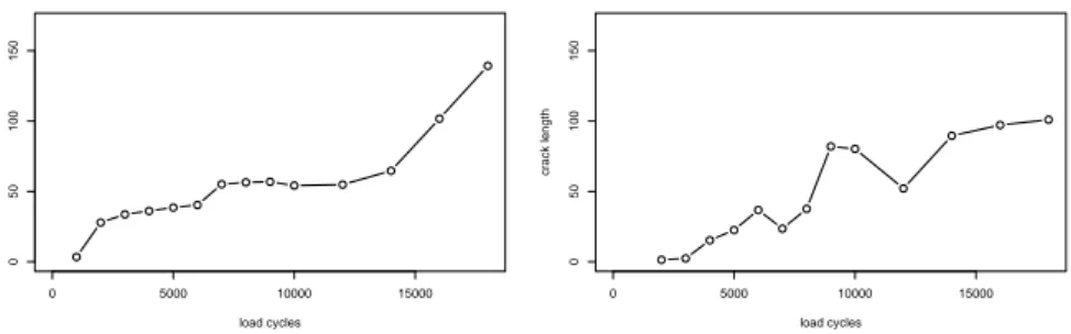
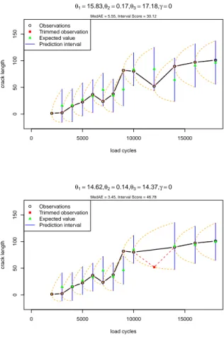
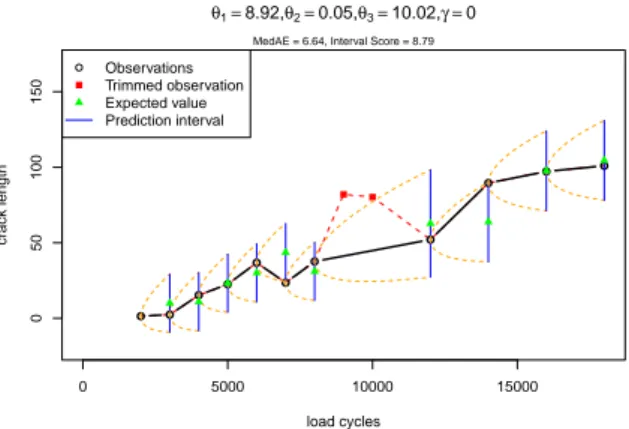
3.2 Performance measures for the crack growth data

Figure 7 shows the predicted (expected) values and prediction intervals us- ing the classical untrimmed maximum likelihood estimator for an Ornstein- Uhlenbeck process (OU) for the path on the right-hand side of Figure 5. This path is not monotone because of extreme outlying observations. These outliers cause bad fits for the Ornstein-Uhlenbeck process using the classical maxi- mum likelihood estimator so that the performance measure MedAE is equal to 5.55 and the performance measure based on the interval score IS

is 30.12.

Using an 10%-trimmed estimator leads to the result shown in Figure 8 with

improved MedAE of 3.45 because one observation is trimmed. However, the

Fig. 9 20% trimmed pre- dicted (expected) values and prediction intervals using an OU model for the curve on the right-hand of Figure 5

0 5000 10000 15000

050100150

θ1=8.92,θ2=0.05,θ3=10.02,γ =0

load cycles

crack length

● ●

●

●

●

●

●

●

●

● ●

● Observations Trimmed observation Expected value Prediction interval

MedAE = 6.64, Interval Score = 8.79

performance measure based on the interval score has increased to 48.78 since the prediction intervals became smaller so that the 7’th prediction interval is more far away from the observed value as for the untrimmed estimator. If 20%, i.e. two observations, are trimmed then the performance measure based on the interval score has decreased to the very small value of 8.79 since all predic- tion intervals include the observations as seen in Figure 9. However, here the MedAE is worse than for using the untrimmed estimator. This extreme exam- ple shows that trimming some few observations improve the two performance measures differently. Here a higher trimming rate is necessary to improve both performance measures simultaneously.

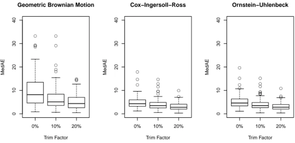
However, the most crack growth curves are not so contaminated as that one on the right-hand side of Figure 5. 20% trimming and even 10% trimming lead to reasonable fits of an Ornstein-Uhlenbeck process, a Cox-Ingersoll-Ross process, or a Geometric Brownian Motion for the majority of the 100 crack growth curves which are backtracked from the 100 largest detected cracks at the end. This can be seen from the boxplots in Figure 10 for the 100 obtained performance measures based on the median absolute deviation (MedAD) and in Figure 11 for the 100 obtained performance measures IS

based on the interval score. Thereby 20% trimming leads to the best result for both perfor- mance measure and this is independent whether an Ornstein-Uhlenbeck pro- cess, a Cox-Ingersoll-Ross process, or a Geometric Brownian Motion is fitted.

However, the Geometric Brownian Motion provides the largest performance

meausure while the performance measures for the Ornstein-Uhlenbeck process

and the Cox-Ingersoll-Ross process are very similar. The same result was ob-

●●

●

●

●

●

●●

●

●●

●

0% 10% 20%

010203040

Geometric Brownian Motion

Trim Factor

MedAE

●

●

●

●●

●

●

●

●

●

●

0% 10% 20%

010203040

Cox−Ingersoll−Ross

Trim Factor

MedAE

●●

●

●

●

●●

●

●

●

●

●

●

●

●

0% 10% 20%

010203040

Ornstein−Uhlenbeck

Trim Factor

MedAE

Fig. 10 Boxplots of the median absolute deviations (MedAD) of the growth curves of the 100 largest cracks in Specimen 31 fitted by three SDEs without trimming, 10% trimming and 20% trimming

●

●

● ●

●

●

●

●

●

●

●

●●

●

0% 10% 20%

020406080100120140

Geometric Brownian Motion

Trim Factor

Interval Score ●

●

●●

●

●●

●

●

●

●●

●●

●●

●

0% 10% 20%

020406080100120140

Cox−Ingersoll−Ross

Trim Factor

Interval Score ^●●

●●

●

●

●

●

●

●

●

●●

●

0% 10% 20%

020406080100120140

Ornstein−Uhlenbeck

Trim Factor

Interval Score

Fig. 11 Boxplots of the interval score IS0.05of the growth curves of the 100 largest cracks in Speci- men 31 fitted by three SDEs without trimming, 10% trimming and 20% trimming

tained when the method was applied to a series of photos of another specimen (Specimen 10) which was exposed to lower stress so that photos are availabe at 29 time points and the crack growth curves are more flat.

The boxplots indicate that the performance measures of the growth curves of

the 100 largest cracks do not follow a normal distribution which was also con-

firmed by Shapiro-Wilk tests. Therefore, to test whether the trimming improve

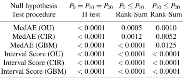
the performance, a closed testing principle based on the H-test (Kruskal-Wallis test) and followed by two Wilcoxon rank-sum tests (Mann-Whitney U-tests) was applied. Table 1 clearly shows that there is a significant difference be- tween no trimming, 10% trimming, and 20% trimming for both performance measures and all three regarded processes. Again only the results for Specimen 31 are presented in Table 1. But for Specimen 10, the P-values are either the same or even smaller.

Table 1 P-values of H-tests and Wilcoxon-Rang-Sum tests for the performance measures obtained from Specimen 31 based on no trimmimg (P0), 10% trimming (P10), and 20% trimming (P20)

Null hypothesis P0=P10=P20 P0≤P10 P10≤P20

Test procedure H-test Rank-Sum Rank-Sum MedAE (OU) <0.0001 0.0005 0.0010 MedAE (CIR) <0.0001 0.0012 0.0052 MedAE (GBM) <0.0001 <0.0001 0.0125 Interval Score (OU) <0.0001 <0.0001 <0.0001 Interval Score (CIR) <0.0001 <0.0001 <0.0001 Interval Score (GBM) <0.0001 <0.0001 <0.0001

Table 2 provides the P-values of a closed testing principle based on the H- test and followed by two Wilcoxon rank-sum tests for testing the equality of the performance measures for the three processes if 20% trimming is used. As in- dicated by the boxplots, there is no significant different between the Ornstein- Uhlenbeck process and the Cox-Ingersoll-Ross process where both differ sig- nificantly from the Geometric Brownian Motion. The results are shown for Specimen 31 but are the same for Specimen 10.

Table 2 Comparison between the performance measuresPOU, PCIR, PGBM applied to the three stochastic processes with 20% trimming in Specimen 31

Nullhypothesis Test MedAE Interval Score POU=PCIR=PGBM H-Test <0.0001 <0.0001

P_OU=P_CIR Rank-Sum 0.8498 0.6087 P_OU=P_GBM Rank-Sum<0.0001 <0.0001 PCIR=PGBM Rank-Sum<0.0001 <0.0001

Finally, it was tested whether the three parameters of the processes with

best fit with 20% trimming, i.e. the Ornstein-Uhlenbeck process and the Cox-

Ingersoll-Ross, are different for the two specimens. The estimated parameters

are given in Table 3 and the test results in Table 4. This shows that there is no significant different in the drift term θ

where the slope term θ

and the diffusion term θ

are significantly higher for higher stress. Note that Sepcimen 10 was exposed to an external stress of 360 MPa and Specimen 31 to 400 MPa.

Table 3 Median of the estimated parameters of the Ornstein-Uhlenbeck processes and the Cox- Ingersoll-Ross processes using 20% trimming for Specimens 10 and 31

Specimen (Process) med(θˆ1)med(θˆ2)med(θˆ3) 10 (OU) 2.2779 0.0814 1.6697 31 (OU) 6.4637 0.0799 3.4209 Difference -4.1858 0.0016 -1.7512

10 (CIR) 2.0858 0.0709 0.4636 31 (CIR) 6.5832 0.0985 0.7547 Difference -4.4974 −0.0275 -0.2911

Table 4 P-values for a two-sided Wilcoxon-Rank-Sum test in order to check whether the estimated parameters are significantly different between Specimens 10 and 31 for the Ornstein-Uhlenbeck pro- cess and the Cox-Ingersoll-Ross process.

Nullhypothesis θ₁⁽¹⁰⁾=θ₁⁽³¹⁾θ₂⁽¹⁰⁾=θ₂⁽³¹⁾θ₃⁽¹⁰⁾=θ₃⁽³¹⁾ Ornstein-Uhlenbeck <0.0001 0.5486 <0.0001 Cox-Ingersoll-Ross <0.0001 0.9229 <0.0001

4 Discussion

We introduced trimmed likelihood estimators for processes given by stochas- tic differential equations and showed how they can be computed efficiently.

To study their performance on a large data set, we proposed an automatic de-

tection method to obtain crack growth data from a series of photos by back-

tracking large cracks detected in the last photo. The application of the trimmed

likelihood estimators to these data showed that these estimators can deal with

a high amount of contamination of the data caused by the automatic detection

method. In particular, the fits of obtained 100 crack growth curves measured

by two proposed performance measures were significantly better for trimming 20% than 10% of the data of a growth curve. For simplicity, only the fits of the Ornstein-Uhlenbeck process, the Cox-Ingersoll-Ross process, and the Ge- ometric Brownian Motion were studied. But similarly other processes can be fitted. Within the regarded three processes, the Ornstein-Uhlenbeck process and the Cox-Ingersoll-Ross process provided the best fits and estimated pa- rameters which differ significantly between different stress conditions. Hence the influence of the stress conditions on these parameters maybe used in fu- ture work to predict the damage development of material by analyzing cracks detected from photos as described in this paper.

AcknowledgementsThe research was supported by the DFG Collaborative Research Center SFB 823Statistical modeling of nonlinear dynamic processes.

References

Beskos A, Papaspiliopoulos O, Roberts GO, Fearnhead P (2006) Exact and computationally efficient likelihood-based estimation for discretely ob- served diffusion processes. Journal of the Royal Statistical Society Series B 68:333–382

Buckley M, Yang J (1997) Regularised shortest-path extraction. Pattern Recog- nition Letters 18:621–629

Castillo E, Fernández-Canteli A (2009) A Unified Statistical Methodology for Modeling Fatigue Damage. Springer, Dordrecht

Cheng TC, Biswas A (2008) Maximum trimmed likelihood estimator for mul- tivariate mixed continuous and categorical data. Computational Statistics &

Data Analysis 52:2042–2065

Cheu YF (1984) Automatic crack detection with computer vision and pattern recognition of magnetic particle indications. Materials Evaluation 42:1506–

1510, 1514

Chiquet J, Limnios N, Eid M (2009) Piecewise deterministic Markov processes applied to fatigue crack growth modelling. Journal of Statistical Planning and Inference 139:1657–1667

Fletcher DI, Franklin FJ, Kapoor A (2003) Image analysis to reveal crack de- velopment using a computer simulation of wear and rolling contact fatigue.

Fatigue & Fracture of Engineering Materials & Structures 26:957–967

Fujita Y, Mitani Y, Hamamoto Y (2006) A method for crack detection on a con- crete structure. Proceedings - International Conference on Pattern Recogni- tion 3:901–904

Gneiting T, Raftery AE (2007) Strictly proper scoring rules, prediction, and estimation. Journal of the American Statistical Association 102(477):359–

378

Gunkel C, Stepper A, Müller AC, Müller CH (2012) Micro crack detection with Dijkstra’s shortest path algorithm. Machine Vision and Applications 23:589–601

Hadi AS, Luceño A (1997) Maximum trimmed likelihood estimators: a uni- fied approach, examples, and algorithms. Computational Statistics & Data Analysis 25:251–272

Hermann S, Ickstadt K, Müller CH (2016a) Bayesian prediction for a jump diffusion process with application to crack growth in fatigue experiments.

Reliability Engineering and System Safety DOI 10.1016/j.ress.2016.08.012 Hermann S, Ickstadt K, Müller CH (2016b) Bayesian prediction of crack growth based on a hierarchical diffusion model. Applied Stochastic Mod- els in Business and Industry 32:494–510

Höök LJ, Lindström E (2016) Efficient computation of the quasi likelihood function for discretely observed diffusion processes. Computational Statis- tics & Data Analysis 103:426–437

Iacus SM (2008) Simulation and Inference for Stochastic Differential Equa- tions. With R Examples. Springer, New York

Iyer S, Sinha SK (2005) A robust approach for automatic detection and seg- mentation of cracks in underground pipeline images. Image and Vision Computing 23:921–933

Kustosz CP, Müller CH (2014) Analysis of crack growth with robust, distribution-free estimators and tests for nonstationary autoregressive pro- cesses. Statistical Papers 55:125–140

Lin YK, Yang JN (1983) On statistical moments of fatigue crack propagation.

Engineering Fracture Mechanics 18:243–256

Müller CH (2016) Software-Pakete / Software Packages. Fakultät Statistik, Technische Universität Dortmund, URL https://www.statistik.

tu-dortmund.de/1253.html

Müller CH, Neykov N (2003) Breakdown points of trimmed likelihood esti-

mators and related estimators in generalized linear models. Journal of Sta-

tistical Planning and Inference 116:503–519

Müller CH, Gunkel C, Denecke L (2011) Statistical analysis of damage evolu- tion with a new image tool. Fatigue & Fracture of Engineering Materials &

Structures 34:510–520

Müller CH, Szugat S, Celik N, Clarke BR (2016) Influence functions of trimmed likelihood estimators for lifetime experiments. Statistics 50:505–

524

Neykov N, Müller CH (2003) Breakdown point and computation of trimmed likelihood estimators in generalized linear models. In: Dutter R, Filzmoser P, Gather U, Rousseeuw PJ (eds) Developments in Robust Statistics, Physica- Verlag, Heidelberg, pp 277–286

Neykov N, Filzmoser P, Dimova R, Neytchev P (2007) Robust fitting of mix- tures using the trimmed likelihood estimator. Computational Statistics &

Data Analysis 52:299–308

Neykov N, Filzmoser P, Neytchev P (2014) Ultrahigh dimensional variable se- lection through the penalized maximum trimmed likelihood estimator. Sta- tistical Papers 55:187–207

Nicholson DW, Ni P, Ahn Y (2000) Probabilistic theory for mixed mode fa- tigue crack growth in brittle plazes with random cracks. Engineering Frac- ture Mechanics 66:305–320

Ortiz K, Kiremidjian AS (1988) Stochastic modeling of fatigue crack growth.

Engineering Fracture Mechanics 29:317–334

Pastorello S, Rossi E (2010) Efficient importance sampling maximum likeli- hood estimation of stochastic differential equations. Computational Statis- tics & Data Analysis 54:2753–2762

Pedersen AR (1995) A new approach to maximum likelihood estimation for stochastic differential equations based on discrete observations. Scandina- vian Journal of Statistics 22:55–71

Pook L (2000) Linear Elastic Fracture Mechanics for Engineers: Theory and Application. WIT Press, Southhampton

Purcell D (1983) Automatic crack detection. Sensor Review 3:130–131 R Core Team (2015) R: A Language and Environment for Statistical Comput-

ing. R Foundation for Statistical Computing, Vienna, Austria, URL https:

//www.R-project.org/

Ray A, Tangirala S (1996) Stochastic modeling of fatigue crack dynamics for on-line failure prognostics. IEEE Transactions of Control Technology 4:443–451

Rousseeuw PJ (1984) Least median of squares regression. Journal of the Amer-

ican Statistical Association 79:871–880

Rousseeuw PJ, Driessen K (2006) Computing LTS regression for large data sets. Data Mining and Knowledge Discovery 12:29–45

Rousseeuw PJ, Leroy AM (1987) Robust Regression and Outlier Detection.

John Wiley, New York

Sánchez-Silva M, Klutke GA (2016) Reliability and Life-Cycle Analysis of Deteriorating Systems. Springer, Heidelberg

Sobczyk K, Spencer BF (1992) Random Fatigue. From Data to Theory. Aca- demic Press, Boston

Sørensen H (2004) Parametric inference for diffusion processes observed at discrete points in time: a survey. International Statistical Review 72:337–

354

Sun L, Lee C, Hoeting JA (2015) A penalized simulated maximum likelihood approach in parameter estimation for stochastic differential equations. Com- putational Statistics & Data Analysis 84:54–67

Virkler D, Hillberry B, Goel P (1979) The statistical nature of fatigue crack propagation. Journal of Engineering Materials and Technology 101:148–

153

Wilcox CD, Dove SB, McDavid WD, Greer DB (2016) UTHSCSA Image Tool. Department of Dental Diagnostic Science, University of Texas Health Science Center, San Antonio, URL http://compdent.uthscsa.

edu/dig/itdesc.html

Wu WF, Ni CC (2004) Probabilistic models of fatigue crack propagation and their experimental verification. Probabilistic Engineering Mechanics 19:247–257

Yamaguchi T, Hashimoto S (2010) Fast crack detection method for large-size concrete surface images using percolation-based image processing. Machine Vision and Applications 21:797–809

Zárate BA, Caicedo JM, Yu J, Ziehl P (2012) Bayesian model updating and

prognosis of fatigue crack growth. Engineering Structures 45:53–61