spin-orbit fields
Dissertation
zur Erlangung des Doktorgrades der Naturwissenschaften (Dr. rer. nat.)
der Fakultät für Physik der Universität Regensburg
vorgelegt von Robert Islinger
aus Regensburg
im Jahr 2019
Die Arbeit wurde angeleitet von: Prof. Dr. Christian H. Back Prüfungsausschuss: Vorsitzende:
1. Gutachter:
2. Gutachter:
weiterer Prüfer:
PD Dr. M. Marganska- Lyzniak
Prof. Dr. C. H. Back Prof. Dr. D. Weiss Prof. Dr. D. Bougeard
1 Introduction 3
2 Theoretical background 7
2.1 Magnetic energy terms . . . 7
2.2 Landau-Lifschitz-Gilbert (LLG) equation . . . 9
2.3 Spin-orbit coupling related effects (I) - FM/NM bilayer . . . 11
2.3.1 Spin current and diffusion . . . 12
2.3.2 Spin Hall effect (SHE) . . . 13
2.3.3 Interface effects and torques . . . 13
2.4 Spin-orbit coupling related effects (II) - Fe/GaAs system . . . 15
2.4.1 Crystal structure and anisotropy . . . 15
2.4.2 Bychkov-Rashba effect . . . 17
2.4.3 Spin-orbit fields and torques . . . 19
2.5 Magnetization dynamics - ferromagnetic resonance (FMR) . . . . 20
2.6 Spin waves in thin ferromagnetic films . . . 24
2.6.1 Spin wave geometry and dispersion relation . . . 24
2.6.2 Lateral confinement . . . 26
2.7 Magneto-optical Kerr effect (MOKE) . . . 28
3 Experimental techniques 29 3.1 Layer growth and sample fabrication . . . 30
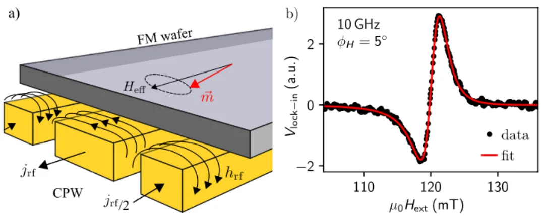
3.2 Electrical detection technique . . . 31
3.2.1 Experimental setup . . . 33
3.2.2 Creation of the rf-driving field . . . 33
3.2.3 Full-film FMR characterization . . . 35
3.2.4 Voltage rectification . . . 36
3.2.5 Spin-transfer torque FMR (ST-FMR) . . . 38
3.2.6 Spin-orbit torque FMR (SOT-FMR) . . . 39
3.2.7 Modulation of damping (MOD) . . . 40
3.3 Time-resolved magneto-optical Kerr effect microscope . . . 41
3.4 Operation modes . . . 44
3.4.1 Spin wave spectroscopy . . . 44
3.4.2 Spin wave imaging . . . 46
3.5 Confinement of spin waves . . . 46
3.5.1 Longitudinally magnetized stripes . . . 46
3.5.2 Transversely magnetized stripe . . . 49
3.6 Static equilibrium change method . . . 51
3.6.1 Simplified TRMOKE setup . . . 51
3.6.2 Theoretical background . . . 52
3.6.3 Determining the spin-orbit fields . . . 53
3.7 Micromagnetic simulations . . . 56
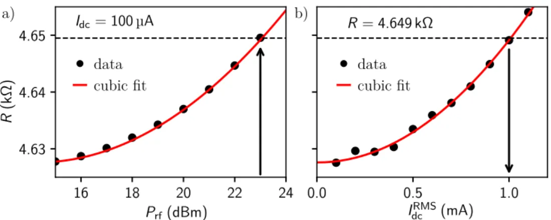
3.8 Bolometric current calibration . . . 56
4 Experimental detection of spin-orbit torques in a Py/Pt bilayer 59 4.1 Magnetic properties . . . 60
4.2 Experimental results . . . 61
4.2.1 Spin-transfer torque FMR . . . 61
4.2.2 Electrical modulation of damping . . . 64
4.2.3 Discussion of results . . . 65
4.2.4 Temperature dependence of the torque ratio . . . 67
4.3 Static equilibrium change method . . . 68
5 Electrical detection of spin-orbit fields in the Fe/GaAs system 73 5.1 Sample layout and magnetic characterization . . . 74
5.2 Electrical detection principle . . . 76
5.3 Calculation of magnetization angle and susceptibility . . . 77
5.4 Determination of spin-orbit fields by SOT-FMR . . . 80
5.4.1 In-plane SOFs . . . 80
5.4.2 Out-of-plane SOFs . . . 85
5.5 Discussion of results . . . 86
6 Optical detection of spin-orbit fields in the Fe/GaAs system 91 6.1 Static equilibrium change method . . . 91
6.2 Dynamic determination by standing spin waves - DE geometry . 92 6.2.1 Sample layout . . . 93
6.2.2 Phase determination . . . 94
6.2.3 Homogeneous excitation of SSWs . . . 96
6.2.3.1 Characterization of DE-CPW SSWs . . . 96
6.2.3.2 Mode pattern . . . 98
6.2.4 Current-driven standing spin waves . . . 99
6.2.4.1 Characterization of the current-driven SSWs . . 100
6.2.4.2 Current-induced mode pattern . . . 101
6.2.4.3 Discussion of results . . . 104
6.2.4.4 Evaluation of the eigenmodes . . . 104
6.3 Standing spin waves in the BV geometry . . . 107
7 Summary 111
Bibliography 115
Acknowledgment 125
Publication list 127
Introduction 1
In recent years, great efforts have been made in solid state physics and especially in the understanding of spin-dependent phenomena [1]. The charge and spin degree of the electron opens a large research area considering applications in the storage information technology, known as spintronics [2]. The fast and efficient way of the generation, detection and manipulation of spin-polarized currents is a crucial goal for future spintronic devices. A large information density, low usage power and non-volatility are required for these devices which is already realized in the STT-MRAM1 [3, 4]. There, the magnetization in one ferromagnetic (FM) layer is manipulated by a spin-transfer torque from a second FM layer due to the transfer of angular momentum from a spin-polarized current through an oxide tunnel barrier. If the current is sufficiently large, it can switch the magnetization. A degeneration of the tunnel barrier due to the large currents leads to a continuous research for new material systems and other ways to overcome this problem [5]. In the field of data storage technology, a main goal is to store more information on smaller areas, increase the device speed and with less cost of energy. Further, the data should be stored without losing information over time. Pushing the lower border in wafer fabrication down with newer lithography steps to several nanometers, heating effects become even more significant due to the high current densities.
Therefore, the conversion of a charge into a spin current became an enor- mous interest in recent years due to the possible applications for spintronic devices. In a bilayer, consisting of a ferromagnet and a non-magnetic metal (NM), different effects cause a conversion of charge into spin current. These arise from the spin-orbit interaction in the bulk NM or at the interface of the hybrid structure, and are known as the spin Hall, Rashba-Edelstein or inverse spin galvanic effect. A transverse spin current with respect to the charge cur- rent direction is generated independently of the type of non-magnetic material, which could be a normal metal [6], topological insulator [7] or a semiconductor [8]. The transverse spin current induces spin-orbit fields (SOFs) which manip- ulate the magnetization in the FM layer. The dynamics can be described by extending the equation of motion for the magnetization vector. An attempt to find the most efficient way to create spin currents is achieved by tuning the ma- terial parameters. However, a reliable method, to determine the strength and
1spin-transfer-torque magnetoresistive random access memory
symmetry of these SOFs, is crucial for the understanding and characterization of the spin-orbit fields.
There are several realized approaches which can be classified into two time scales: static and dynamic experiments. A quasi static method is the so-called two-omega method, where the SOFs are determined by the first and second har- monic Hall resistance at low frequencies for different magnetic field configura- tions [9]. Another dc-based method has recently been proposed, where the equi- librium position of the magnetization is altered by a low frequency ac-current [10, 11]. The displacement can be detected optically using the magneto-optical Kerr effect (MOKE). However this method is limited to materials showing not a too large in-plane magnetization. For this reason, the excitation in the ex- periments presented in this thesis is chosen in microwave frequency range and the SOFs can be detected with the help of the ferromagnetic resonance (FMR) technique. The precession of the magnetization is driven by a spin transfer torque (ST-FMR) from a spin current or by a spin-orbit fields (SOT-FMR) originating from the current flow through a conducting sample. In both cases, the rectified dc-voltage is carefully analyzed with respect to the magnetization angle in order to quantify the interface-induced SOFs. The strength and sym- metry are derived for a single crystalline Fe/GaAs(001) system [8], where it is possible to tune the SOFs magnitude by a gate voltage [12]. The investigated Fe/GaAs(001) provides efficient SOFs as well as an ultra low damping compared to many FM/NM bilayers [13].
Furthermore, in this thesis, a new approach is demonstrated, where the SOFs can be determined optically by using time-resolved magneto-optical Kerr effect microscopy (TRMOKE) using the same excitation procedure as for the SOT-FMR method. Thereby, the impact of the SOFs on the magnetization dynamics is utilized to determine the SOFs in a very efficient manner. Moreover, this method is self-calibrated since the magnitude of the SOFs is compared to the effect of the current-induced Oersted field. Further, spurious effects from a rectifying dc-voltage can be neglected due to the direct optical measurement of the polar component of the magnetization. The experimental results are compared to micromagnetic simulations which include all contributing fields.
The thesis is organized as follows: Ch. 2 begins with the theoretical back- ground which contains the different energy terms in the ferromagnet and are used to describe the dynamical motion of the magnetization vector by the Landau-Lifshitz-Gilbert (LLG) equation. The SOF related effects, arising in the two investigated material systems, are also introduced, and extend the LLG equation by two additional terms. The basic principle of the precessional motion of the magnetization by excitation in the microwave frequency range causing ferromagnetic resonance is discussed. The concept of spin waves is in- troduced together with the influence by a lateral confinement in a FM stripe and the magneto-optical Kerr effect. Ch. 3 explains the electrical and optical
ends with a discussion of two possible geometries for standing spin waves and a description of the basic principles of micromagnetic simulations. In Ch. 4, the conversion efficiency from a charge to a spin current is derived by ST-FMR for a Py/Pt bilayer. The spin Hall angle and the spin diffusion length are extracted from a platinum thickness dependence, and the results are compared to those from other techniques and material systems. In Ch. 5, the Bychkov-Rashba- and Dresselhaus-like spin-orbit fields are derived for the Fe/GaAs(001) system by the electrical SOT-FMR method along the different crystallographic axes of the GaAs. The last chapter explains the new optical approach where a unique mode pattern of standing spin waves is generated by an inhomogeneous driving torque. The resulting mode pattern can be compared to micromagnetic simu- lations to extract the SOFs which are in turn compared to the values obtained from the electrical method. At the end, the thesis concludes with a summary of all results.
Theoretical background 2
In order to describe the magnetic system, it is necessary to introduce first the magnetic energy contributions relevant for the magnetization in the sample. By exciting the magnetization vector in a proper way, it starts to precess around an equilibrium position and then undergoes ferromagnetic resonance under certain conditions. The motion can be modified by magnetic fields or additional torques arising from an injected current. The dynamics of the magnetization vector are in general described by the Landau-Lifshitz-Gilbert equation. In order to account for the dynamics, the ferromagnetic resonance is discussed which happens under particular conditions. Then, two important effects are treated which arise for the two investigated material system. Finally, the concept of spin waves is introduced, where the confinement by a simple stripe leads to the emergence of standing spin waves.
2.1 Magnetic energy terms
Magnetism, on a quantum mechanical level, can be described as an ensem- ble of interacting magnetic moments where the influence of every moment on the nearest neighbors is considered. A micromagnetic description of the ferro- magnet includes different spatial scales in a continuum theory [14]. The local magnetization at every lattice point is represented by a vector field M(r, t) with space coordinaterand timet[15]. The strong exchange interaction domi- nates on a small spatial scale below the Curie temperature1, which is consistent with the continuum approximation due to the discrete nature of the lattice.
The sum of all spins can be substituted by an integral over the vector field.
One fundamental constraint is the conservation of the magnitude of the local magnetization
|M(r, t)|=MS, (2.1) which is equal to the spontaneous or saturation magnetization on every point in the ferromagnet. The vector field normalized by MS leads to a reduced magnetic moment or unit vectorm(r, t). Simply, mis used in the following as the magnetization vector and simplifies micromagnetic simulations on a grid.
1A threshold temperature, above which a ferromagnet becomes paramagnetic. For the 3d ferromagnetic (FM) materials used in this thesis, this is about 1043 K for Fe, 631 K for Ni [14] and 871 K for Permalloy (Py, Ni80Fe20) [16].
The micromagnetic free energyGLof the system in a volumeV is expressed by [14]
GL(m,Hext) =Z
V
A(∆mx)2+ (∆my)2+ (∆mz)2 +fani(m)−µ0MS
2 m·Hdem−µ0MSm·Hext
dV. (2.2) Here, only terms are involved which are necessary to describe the ferromagnet:
the first term represents the exchange energy which increases for canted mag- netization vectors between nearest neighbors. The exchange stiffness constant A is on the order of 10−11J/m for a ferromagnet. The second term describes the crystal anisotropy energy which is explained in the following in more detail.
The third and the last terms contribute to the magnetostatic and external ap- plied fields, respectively. The magnetostatic field Hdem is determined by using the Maxwell equations in order to account for the charges at the surface of the ferromagnet.
In single-crystalline samples, the so-called magneto-crystalline anisotropy leads in general to energetically favored directions for the magnetization. In the case of 3d ferromagnets, the 3d orbitals are partially filled, however, the orbital moments are almost quenched by the crystal field with a small orbital moment left. Due to spin-orbit coupling, the spin moment is coupled to the residual orbital moment and hence to the lattice arrangement leading to an energy density with the same symmetry as the crystal [1]. With the projections of the magnetization onto unit vectors of the crystal αi = m·ˆei, the energy density for a cubic system can be given in lowest order as [17]
E4-fold=K4(α2xα2y+α2yα2z+α2xα2z) = K4
2 (1−α2x+α2y+α2z), (2.3) with K4 as the cubic or four-fold crystalline anisotropy constant. In the used Fe/GaAs system, an additional uniaxial in-plane (ip) component arises from an Fe/GaAs interface and causes a two-fold symmetry [18]. Further, a uniaxial out-of-plane (oop) term is generated by reducing the iron film thickness down to a few nanometers [17]. The resulting energy with only first order terms then reads [19]
Eani =−K4k
2 (α4x+α4y)−K4⊥
2 α4z−Kunik (ˆn·m)2
MS2 −Kuni⊥ α2z (2.4) with Kunik and Kuni⊥ as the ip and oop uniaxial anisotropy constant, respec- tively. Here, the unit vector ˆn points along the uniaxial anisotropy direction.
In this thesis, a compound of nickel and iron, named permalloy (Py), is inves- tigated, which consists of 80% nickel and 20% iron atoms. The ratio of this alloy is designed to compensate the four-fold and uniaxial magneto-crystalline
anisotropies. Due to the small coercive field, this type of ferromagnet is often called soft magnetic because the anisotropies vanish [20].
The equilibrium state of the ferromagnetic system for a given externally applied magnetic field is found at δGL = 0 while varying the magnetization vectorm and calculating the change in the Gibb’s free energy Eq. (2.2). This issue was expressed by Brown [15]
m×Heff = 0, (2.5)
where the torque between the magnetization and an effective field must be zero.
The effective fieldHeff is the sum of the four individual fields in Eq. (2.2) Heff=Hex+Hani+Hdem+Hext, (2.6) where each field can be derived by the variation of the energy with respect to the magnetizationm.
2.2 Landau-Lifschitz-Gilbert (LLG) equation
The response of the system after excitation is a more interesting topic to ex- amine. After experiencing a perturbation away from the equilibrium position, the temporal observation of the magnetization dynamics can used to further understand the magnetic properties. For a non-zero torque m×Heff 6= 0, the system is no longer in the equilibrium position and evolves in time due to the prevailing dynamics.
The spatial and temporal evolution ofmcan be explained in the following within a relaxation process. Gilbert proposed an equation of motion for the magnetization vector [21]
dm
dt =−γm×µ0Heff+αm×dm
dt =Teff+Tdamp, (2.7) when it gets tilted out-of-the equilibrium state by a perturbation including a damping mechanism. Here, γ is noted a precession rate or the gyromagnetic ratio, which is given by γ = g|e|/(2me) with the Landé factor g, the electron charge e and the mass me. The second terms exhibits a phenomenologically introduced Gilbert damping parameterα [22]. The expression can be split up into two parts, namely a precessional term which exerts an effective field-like torqueTeff and a damping-like torqueTdamp on the magnetization.
The first term of Eq. (2.7) induces a precession of the magnetization vec- tor around an effective magnetic field Heff which is introduced in Eq. (2.5).
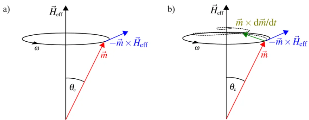
Fig. 2.1(a) sketches the precessional motion of m on a cone around Heff at an angle θc with an angular frequency ω = 2πf. For a free electron, typical precession frequencies are in the range of several gigahertz (GHz). The equi- librium condition is specified by meq ×Heff = 0 and aligns the equilibrium
a) b)
Figure 2.1: The trajectory of the magnetization vector around an effective fieldHeff
with only the precession term a) and with an additional damping term b). The first term in Eq. (2.7) describes the precessional motion aroundHeff at a frequencyω. The second term tries to align m parallel to Heff in the equilibrium position and leads finally to a spiral trajectory towards the equilibrium position along the effective field.
magnetization with the effective field. For any non-collinearmwith respect to Heff, a driving torque Teff leads to a precessional motion around the effective field. This would keep going forever and preserves the total energy, which is unphysical.
Therefore, a damping term accounts for the loss of energy, which is propor- tional to the precession velocity [23]. A proportionality factor α, the so-called Gilbert damping parameter, denotes the strength of the phenomenologically introduced term. This quantity refers to the intrinsic magnetic damping, is dimensionless and material dependent. The damping-like torque tries to align the magnetization parallel along the effective field due to the cross product m×dm/dt. Fig. 2.1(b) shows the trajectory of m moving on a spiral curve (dashed line) towards the effective fieldHeff.
Additional torques can be generated for instance by electrical currents in heterostructures like a ferromagnetic metal/normal metal (FM/ NM) or ferro- magnetic metal/semiconductor (FM/SMC) bilayer. Those torques are added to the LLG and will affect the magnetization dynamics in different ways. In this thesis, two current-induced torques will manipulate the magnetization:
• the spin-transfer torque (STT) caused by a transfer of angular momentum originating from a spin current, theoretically predicted by Berger [24] and Slonczewski [25].
• the spin-orbit torque (SOT) generated by a spin accumulation at an inter- face due to the spin-orbit coupling [1, 9].
Since |M| = MS holds, these torques can be split into two orthogonal parts
with respect to the previously defined effective field. They read
TFL =−γτFLm×σFL, (2.8)
TDL=γτDLm×(m×σDL), (2.9) with σFL,DL as the unit vector of spin-polarization direction and τFL,DL as strength of the underlying torques [22]. The torque TFL in Eq. (2.8) has the same form as the first term in the LLG and induces a precession of the mag- netization if Hk σFL. Therefore, this term is called field-like torque and acts perpendicular tom. The damping-like torque in Eq. (2.9) shows a double cross product and also generates a torque perpendicular to the magnetization. This conducts to a reduction or enhancement of the former introduced damping torqueTdamp. For this reason, this term is called damping-like torque since it is similar to the second term of Eq. (2.7). The extended LLG equation with the two torques reads:
dm
dt =−γm×(µ0Heff+τFLσFL) +αm×dm
dt +γτDLm×(m×σDL). (2.10) Basically, the magnetization can be manipulated by current-induced torques which are generated by either pure spin currents in the ferromagnetic material via the interface or by spin accumulation. Both field- and damping-like torques originate from the spin-orbit coupling, however, the magnitude and sign depend on the used material. These torques can act onmin two possible ways. First, spin currents enter the ferromagnetic layer through an interface, gets absorbed and transports angular momentum to the FM. Thereby, a damping-like torque acts on the magnetization. Second, a spin accumulation, non-collinear with the magnetization, engages a precession around the local magnetization due to exchange coupling and vice versa [26]. Both torques originate from either a 3D spin-orbit coupling (SOC) effect called spin Hall effect (SHE) or a 2D SOC effect called Rashba-Edelstein effect (REE).
2.3 Spin-orbit coupling related effects (I) - FM/NM bilayer
In this section, the basic concept of spin currents and spin accumulation are discussed for the case of a FM/NM bilayer. Further, the spin Hall effect is introduced, which generates a spin-polarized current in the heavy metal due to the spin-orbit coupling. The transport of angular momentum to the attached ferromagnetic layer causes a torque on the magnetization in the FM and leads to precession ofm. Finally, the properties of the FM/NM interface are discussed in the light of the transmission and absorption of the spin currents.
2.3.1 Spin current and diffusion
Spin-orbit coupling is defined as the interaction of the electron’s spin with the gradient of the electrical field which can be imagined as a magnetic field in the rest frame of the electron due to relativistic effects
HSO= ~
4m2ec2 (∇V ×p)·σ (2.11) with the electrostatic potentialV, the momentumpand the Pauli spin matrices σ.
For example, spin-polarized currents can be generated by a charge current flow in a FM, where different conductivities for spin up and down electrons are present. The difference in electron spins js =j↑−j↓ defines the resulting net spin current next to the normal charge currentjc=j↑+j↓. The spin current can pass an interface to a normal metal or semiconductor, where it is transmitted with a certain efficiency. Away from the interface, the electron current has to be unpolarized js = 0, since the conductivities for both spin are equal. The transfer of spin up and down electrons from the FM to the NM/SMC goes along with an accumulation of spins at the interface by a splitting of the chemical potentials µ↑ and µ↓. The resulting spin accumulation µs = (µ↑ −µ↓)/2 is localized at the interface and decays with the spin diffusion length (SDL) λsd
in the material.
A net spin accumulation of s~/2 can be defined with the net spin particle number s=n↑−n↓ of up and down spins pointing in different directions. The drift-diffusion continuity equation for a spin density is given by [27]
∂s
∂t + ∂
∂x
−µsE−D∂s
∂x
= ∂s
∂t− ∂
∂xJS =−s τs
, (2.12)
where Js denotes the spin particle density, D the diffusion parameter, µ the magnetic moment and τs the spin relaxation time. Assuming a constant spin density ∂s/∂t=E = 0, Eq. (2.12) reduces to
∂2s
∂x2 = s
λ2sd, (2.13)
where the spin diffusion length λsd =√
Dτs quantifies a characteristic distance for a conserved spin transport [1]. The SDL in metals is only several nanometers compared to micrometers in semiconductors [28].
A spatially varying spin density or spin accumulation from a FM/NM inter- face into the FM layer can be mathematically described by the following ex- pression for a spin current density
js(x) =js0exp(− x λNM
) (2.14)
with an initial spin current densityjs0 =−D∂s(x= 0)/∂x atx= 0.
2.3.2 Spin Hall effect (SHE)
The spin Hall effect describes the conversion of a charge current into a transverse spin current in the absence of external magnetic fields by the spin-orbit coupling in a normal metal. The effect was discovered in 1971 by Dyakonov and Perel [29]
and brought back into attention in 1999 by Hirsch [30]. The first observations were made in semiconductors [28], which sparked interest in the research for FM/NM systems. There, the magnetization can be manipulated and switched by injecting charge currents [31–33].
The phenomenon is based on the spin-dependent asymmetric scattering of unpolarized electrons in the NM material. The spin-orbit coupling originates from the band structure of the material (intrinsic) or from impurities (extrinsic) and leads to a coupling between spin and charge currents. Thereby, a transverse pure spin current is created from a charge current and vice versa due to the Onsager principle [34]. Both conversions are connected via the effective spin Hall angleθeffSHA to
jc= 2|e|
~ θeffSHAjs, (2.15)
where the spin Hall angle has values between 0< θSHAeff <1 for FM/NM material system and can be denoted as an effective SHA if a transparent interface is considered. Thereby, a charge current through for example a NM stripe does lead to a spin accumulation at all boundaries perpendicular to the current direction.
Two type of spin currents arise in a thin stripe due to the symmetry of the system with an in-plane charge current flow j = jxx: first, spin currentsˆ in both z directions which are in-plane spin-polarized. Second, two in-plane spin currents along they directions withoopspin-polarization. These four spin currents cause spin accumulation at all interfaces of the stripe. However, only at one interface, one part of the spin accumulation diffuses into the attached FM layer, where the perpendicular component with respect tomgets absorbed.
Thereby, angular momentum is transferred to e.g. a FM film which influences the magnetization dynamics. The torques depend on the bulk properties of the NM as well as on the FM/NM interface. The other part of the spin current is reflected back into the NM layer. Therefore, the interface has also to be taken into account which is discussed in the following.
2.3.3 Interface effects and torques
The torque, generated via the transfer of angular momentum through an inter- face, is the so-called spin transfer torque (ST). It can be decomposed into the two terms [26]
T= γ
τexMSm×s+ γ
τdampMSm×(m×s), (2.16)
depending on the orientation of the cross product. The first term describes the precession of the spin accumulation s around the local magnetization m due to exchange coupling. The second term is perpendicular to this preces- sional motion, which is similar to the previously mentioned damping-like term.
The damping process is fast in the treated metallic ferromagnets and any non- collinear spin accumulation leads to a relaxation of the transverse spin current within a few lattice constants [35]. Therefore, it is justified to assume an in- stant torque at the interface. The relaxation of the collinear spin accumulation occurs by transferring angular momentum to the lattice. Finally, the drift diffu- sion equation from Eq. (2.12) is solved and the resulting damping- and field-like torques are obtained [26]
TFL =γτFLm×σFL, (2.17)
TDL=γτDLm×(m×σDL). (2.18) with the field- and damping-like unit-vector of the spin polarization direction, see Eq. (2.9). The two spin injection efficiencies are given by
τDL,FL =− ~ 2|e|µ0MSdFM
ηFL,DLθSHAeff jc, (2.19) and the magnitude is between 0< ηFL,DL ≤1.
The equation for the current conversion, Eq. (2.15), can be rewritten with a normalized spin Hall angle θnorm = ηDLθSHA by considering the interface of the heterostructure. In order to evaluate the experimental data, an exact knowledge of the interface properties is necessary. Therefore, an expression for the spin injection efficiencyηtrans was proposed [36]
ηtrans =
1− 1 cosh(λdNM
NM)
, (2.20)
which is the first part of a full calculation of the drift diffusion equation with a boundary condition of a vanishing transverse spin accumulation [26]. The interface reflectivityηtransdepends on the thickness of the NM layer in compar- ison to the spin diffusion length of the used material. If the NM layer thickness reaches the spin diffusion lengthλNM,ηtrans saturates due to the cosh-term and the net spin current across the interface stays constant due to the backflow from the NM/substrate interface [37].
Further, two parameters are required for calculating the interface resistance:
first, the effective spin-mixing conductance (SMC) [26]
g↑↓eff=µ0MSdFMeαNM−α0
γ~ , (2.21)
which accounts for the difference of the Gilbert damping parameter between a FM/NM layer and a sample with only a FM layer (α0). And second, the
knowledge of the bulk conductivity of the normal metal layer σ0 is needed, which can be determined by a conductivity measurement.
The resulting expression for the damping-like injection efficiency ηDL can be written as [38]
ηDL= 2e2
hg↑↓effλNM
σNMtanh( dNM
2λNM). (2.22)
A normalized product of the spin injection efficiency and the spin Hall angle can be defined as
(ηDLθSHAeff )norm:=ηDLθSHAi h 2e2
σNM
g↑↓eff =θSHAi λNMtanh dNM
2λNM
, (2.23) where the effective spin Hall angle is normalized by the factor hσNM/2e2g↑↓eff. An interface-related SHAθSHAi is introduced, which can be determined by the fit of a tanh-function in a NM layer thickness dependence. Thereby, also the spin diffusion lengthλNM can be extracted [38–40].
2.4 Spin-orbit coupling related effects (II) - Fe/GaAs system
In this section, the Rashba-Edelstein effect (REE) is discussed [41, 42]. It can be understood as transverse in-plane spin-polarization generated at the interface of a normal metal by application of an electrical field. This effect was first experimentally observed by Kato [43] and Silov [44]. Basically, the Rashba effect can be seen as an effective magnetic field due to the spin-orbit coupling, which is seen by the drifting electrons in their own reference frame [45, 46].
The field generates additional terms in the Hamiltonian and removes the spin degeneracy of the energy bands.
In semiconductors with SOC, the Hamiltonian can be split up into a Dres- selhaus and a Bychkov-Rashba field originating from a bulk (BIA) or structure inversion asymmetry (SIA), respectively. The Hamiltonian finally reads as
H= ~k2
2m∗ +HSOBIA+HSOSIA, (2.24) with the momentum~k2 and the effective mass of the electronm∗.
2.4.1 Crystal structure and anisotropy
One part of thesis was the electrical and optical determination of spin-orbit fields in thin Fe/GaAs stripes. Therefore, the treated material is briefly dis- cussed. Gallium arsenide is a III-V semiconductor and shows a zinc-blende structure with a face-centered cubic (fcc) lattice structure. The diatomic basis contains a Ga and an As atom which can be imaged as an atom in the center of a tetrahedron with four nearest neighbor atoms at the vertex corners [48].
Figure 2.2:Top view of an un- reconstructed GaAs(001) sur- face where the different size of atoms corresponds to the posi- tion of the atomic layers. The lower right section shows the unit cell of the first monolayer of Fe (blue) on the GaAs lattice with the two bonds along the [-110] direction (image taken from [47]).
Fig. 2.2 displays the top view on a GaAs(001) lattice which is not reconstructed during the Fe growth. Every atom is connected by two bonds to the lower and two bonds to the higher lattice plane to the other type of atom.
In GaAs(001), the top layer consists of either only Ga or As atoms, where a single atom shares only two bonds to the lower lattice plane. The other two bonds point into vacuum and are called dangling bonds. They are oriented along the [-110] or [110] crystallographic direction depending on whether the crystal is As- or Ga-terminated interface. For this reason, an intrinsic anisotropy emerges at the surface independent of the termination. Both directions are not equivalent and this results in a two- and four-fold anisotropy which can be described by a C2v point group [49]. A Fe layer grown on GaAs(001) adapts this interface symmetry, since the lowest Fe atoms are bonded to the GaAs(001) by the two dangling bonds [1]. The Fe atoms occupy the same lattice positions since Fe grows epitaxially on GaAs. In detail, the lattice constant of GaAs (aGaAs = 5.653 Å) is almost twice as large as iron (aFe = 2.867 Å), which results in a roughly strain-free and pseudomorphic crystalline growth [50].
In a thin Fe film attached to the GaAs(001), there exists both a cubic magneto-crystalline anisotropy originating from the bulk Fe as well as the pre- viously introduced uniaxial magneto-crystalline anisotropy from the Fe/GaAs interface. The anisotropy energy from Eq. (2.4) for the in-plane case can be rewritten as [51]
ani(φM) = K4k
4 sin2(2φM) +Kunik cos2(φM), (2.25) whereφM defines the angle between the magnetization and the [-110] direction.
The two anisotropy constants K4k and Kunik depend on the FM layer thickness and specify the strength of the four-fold and uniaxial anisotropy, respectively.
The four-fold parameter is negative for films sizes thicker than one nanometer, which favors two easy axes along the [100] and [010] direction. The uniaxial term stems from the bonds of the Fe/GaAs(001) interface and has a positive value,
hh lh CB
hh lh
a) b)
+k' -k'
so k k E E
VB
Figure 2.3:a) The band structure of a III-V semiconductor shows a fundamental gap between conduction and valence band. b) The spin-orbit interaction leads to band- splitting with ∆SO and the subbands are shifted by ±k’ due to the Rashba field (replotted from [1]).
which favors an easy axis along the [110] orientation [52, 53]. The interplay between both anisotropies depends strongly on the film thickness. For a 3.5 nm thin Fe film, the uniaxial anisotropy dominates the four-fold contribution by a factor of about two, which increases for thinner samples, since it originates from the interface.
2.4.2 Bychkov-Rashba effect
The band structure of a III-V semiconductor, as GaAs(001), is sketched in Fig. 2.3. Panel (a) shows the s-type (conduction band (cb), atomic orbital momentum l = 0) and p-type (valence band (vb), l = 1) energy bands. The spin-orbit interaction lifts the three-fold valence band degeneracy into a two- fold generated light (lh) and heavy hole (hh) band and a split-off band (so).
The arising energy gap ∆so is about ∆so≈0.3 eV for GaAs [54].
A confinement of electrons, e.g. along the growth direction, leads to a quan- tization, which lifts the degeneracy of thelh/hhbands, see panel (b). Further, the structure inversion asymmetry from the GaAs(001) zinc-blende structure induces a spin-splitting of the subbands by −∆k and +∆k with respect to k= 0. The effect is called Bychkov-Rashba effect (BR) when spin currents are involved. In the 2D GaAs(001) system, this effect is caused by an asymmetric spin relaxation in a system with lifted spin degeneracy due tok-linear terms in the Hamiltonian [55].
The microscopic origin of the Rashba effect can be explained by the move- ment of a electron with momentum in an electrical potential of a nucleus [1].
With relativistic corrections, the electric field is transformed into an effective magnetic field acting on the spin of the electron via the spin-orbit coupling. If the crystal has broken inversion symmetry, the conduction electrons will expe-
rience a net electric field perpendicular to the interface. The Rashba field is related to an asymmetric crystal field potential V of either the interface (SIA), and the Dresselhaus field to the crystal itself (BIA) [56]. A moving electron in the electric field of this potential feels a magnetic field
BSO,R=− ~
2mec2k×E. (2.26)
It was shown by Vasko [57], Aronov [42] and Edelstein [41] that a charge cur- rent in presence of Rashba Hamiltonian leads to spin polarization of the con- duction electrons in semiconductor [55]. In bulk material with the SHE, the spin accumulation builds up directly at the interface between semiconductor and ferromagnet leading to a coupling of spin accumulation and magnetization generating a torque on m.
The Rashba field gives rise to three types of spin-splittings with different broken symmetries. The first type is the formerly explained Bychkov-Rashba spin-splitting which is predicted for crystals with one high-symmetry axis [58].
This effect is studied mostly in 2D semiconductor heterostructures where the electrons are confined to thexy-plane [45, 56]. The field termHSOSIAin Eq. (2.24) is given by
HBR=αBR(zˆ×k)·σ (2.27) with the Rashba coefficient αBR, the electron wave vector k, the Pauli spin matrixσand the growth directionz, which breaks the symmetry. The so-calledˆ Dresselhaus term links to the bulk inversion asymmetry in bulk zinc-blende crystals. For 2D GaAs(001) system, the Dresselhaus field is proportional to k and k3 [59] and reads
HD=βhσxkx(k2y−kz2) +σyky(k2z−k2x) +σzkz(kx2−k2y)i (2.28) withβ as the strength parameter. The last contribution is present at interfaces with different types of atoms and is called the interface inversion asymmetry
[010]ky [110]
[100]
kx
[-110]
[010]ky [110]
[100]
kx
[-110]
a) b)
Figure 2.4: The Bychkov-Rashba (a) and Dresselhaus (b) spin-orbit fields are plotted as vector fields with respect to the two in-plane components kx,y of the wave vector and the crystallographic axes of GaAs(001).
[010] ky [110]
[100]
kx
[-110]
[010]
[110]
[100]
[-110]
a) b)
Figure 2.5:The combination of both fields shows a uniaxial anisotropy in terms of a vector field plot (a) and polar plot (b), where the Bychkov-Rashba is assumed to be twice as large as the Dresselhaus term.
(IIA) [60]. The IIA causes additional k-linear terms, which can be related to the bulk inversion asymmetry due to the same phenomenological behavior.
Fig. 2.4 plots the Bychkov-Rashba and Dresselhaus fields as vector fields and as a function of the two in-plane wave vectors kx,y. While the spin Hall effect generates a pure spin current and causes a spin accumulation at the edges, the Rashba effect generates a spin accumulation at the interface. The Rashba effect can only be present in gyrotropic media2 resulting in a non-zero average spin polarization [61] by a Rashba or Dresselhaus spin splitting of bands in a gyrotropic media due to a dc-current [55].
2.4.3 Spin-orbit fields and torques
The resulting spin polarization depend on the strength of both structure and bulk inversion asymmetry which induces a uniaxial anisotropy. A Zeeman-like effective term can be derived from the combined Dresselhaus and Bychkov- Rashba field as
Beff(k) = 1 µB
βkx−αBRky αBRkx−βky
!
(2.29) with the corresponding strength parameter.
The superposition of both fields is visualized in Fig. 2.5(a) where a two times larger Rashba contribution is assumed. A two-fold symmetry of the spin- splitting energy can be found where the dominating part is oriented along the [110] direction for a Fe/GaAs(001) system. This originates from the superposi- tion of both BIA and SIA, which can be visualized as a C2v point group.
The spin-splitting energy from the SOI is defined as ∆SO = 2µB|Beff|
2Materials with a space inversion asymmetry and a low symmetry, i.e. the class of C2v- symmetry with Fe/GaAs interface.
where the magnitude is calculated to [1]
|∆SO|= 2kkqαBR2 +β2+ 2αBRβsin(2φk), (2.30) with an in-plane wave vector kk with kx = kkcos(φ) and ky = kksin(φ).
Fig. 2.5(b) depicts the magnitude of the SOC in a polar plot.
The anisotropy axis can be flipped by tuning the Bychkov-Rashba param- eter via a gate voltage or an electron density in a 2DEGs [62] or Fe/GaAs/Au heterojunctions [63]. Furthermore, both interactions can be adjusted in order to cancel out along certain crystallographic directions, which gives rise to inter- esting effects, i.e. the vanishing spin-splitting in certain k directions [64], the lack of Shubnikov-de-Haas oscillations [65], the absence of spin relaxation [66]
and the non-ballistic field-electron transistor [67]. Nevertheless, it is crucial to be able to disentangle both contributions which was done in experiments using the spin galvanic effect [68] and spin-splitting in quantum wells [69].
The previous introduced fields can act as torques on the magnetization in the FM layer, which is discussed in the following. The torque from the Rashba effect can be calculated to [70, 71]
TBR = m∆ex
e~EFαBRm×(ˆz×m), (2.31) where the exchange energy ∆ex = Jex~MS/(2γ) is introduced with the ex- change coupling Jex between spin and magnetization, and Fermi energy EF. This torque can be inserted into the LLG equation, where it acts on the mag- netization like a magnetic field
µ0HBR= αBR 2µBMS
P(ˆz×jc) (2.32)
with the spin polarization P = ∆ex/EF [26, 56]. This field is proportional to the applied current and is important for thin films since it scales inversely with the film thickness. Finally, the field-like torque can be written as
TFL,BR=−γτFL,Rm×σFL,BR (2.33)
with the torque strength
τFL,R =− αBRP
2µBMSjc (2.34)
and spin polarization σFL,BR = ˆy perpendicular to a charge current in x- direction.
2.5 Magnetization dynamics - ferromagnetic resonance (FMR)
This section treats the temporal evolution of the magnetization when it is driven out of the equilibrium position meq by an external applied magnetic driving
x
y z
z' y' x' Figure 2.6: Used measurement system
(x, y, z) is transferred to a new coordi- nate system (x0, y0, z0) where the equilib- rium magnetization is oriented alongmeq= (x0,0,0) in order to calculate the magneti- zation dynamics.
field hrf(t). The precession of m in a resonant manner on a cone around a stable equilibrium position meq is called ferromagnetic resonance (FMR). The response is linear for small deflections from meq and thus, the amplitude is directly proportional to the driving torque strength [72]. At the resonance frequency of the system, the internal frequency of the magnetic moments fulfill the FMR condition and the precession amplitude becomes maximal.
In experiments, the equilibrium condition meq k Heff is perturbed by a periodic excitation via a small, time varying magnetic field hrf(t). This field exerts a torque on the magnetization which tiltsmaway from the effective field (m∦Heff) into a precessional motion. In addition, an external static field Hext
is applied in order to tune the magnetic stiffness of the system. Thereby, the resonance frequency of the system changes within the GHz range. FMR occurs at a certain magnetic resonance field Hres when both driving and resonance frequency coincide. There, the precessional amplitude becomes maximal. The FMR technique is often used to determine magnetic properties, as for example the effective magnetizationMeffand the Gilbert damping parameterα. Notably, a large magneto-crystalline anisotropy, i.e. for iron, changes the magnitude of the resonance field along the different crystallographic axes. Therefore, the FMR technique is also used to derive the anisotropy constants.
The linearized Landau-Lifschitz-Gilbert equation from Eq. (2.7) can be solved around the equilibrium magnetization position by assuming only small deviations expanding the damping term. This procedure was derived in de- tail by Obstbaum and Decker [27, 37], thus only the most important steps are displayed in the following.
All contributing fields, acting as torques on the magnetization, have to be divided into static and dynamic contributions while each of them can be splitted into a field- and damping-like term. First, the equilibrium positionmeq has to be found and expressed in the azimuth angleφand the polar angleθ to
meq =
sin(θ)cos(φ) sin(θ)sin(φ)
cos(θ).
(2.35)
Fig. 2.6 sketches a second coordinate system (x0,y0,z0) in order to apply for meq = ˆx0. The magnetization can be split up into a static and dynamic part
as
m(t) =meq+ ∆m(t) =
1
∆my0(t)
∆mz0(t),
(2.36)
where the magnetization is precessing around meq in the y0z0-plane. Notably, there is no dynamic part along x0 and the change of ∆m is perpendicular to meq. All contributing fields have to be transformed into the local coordinate system with respect to φand θ.
The result from a complex exponential ansatz ∆m(t) = ∆meiωt is lin- earized by discarding higher-order terms. The solution is a set of two equations which can be written in terms of matrix elements with the dynamic suscepti- bilities:
∆my0(t)
∆mz0(t)
!
= χy0y0 χy0z0
χz0y0 χz0z0
!
· wy0
wz0
!
. (2.37)
Here, the in-plane wy0 = (hy0 −τDL/µ0σz0)eiωt and out-of-plane wz0 = (hz0 − τDL/µ0σy0)eiωt driving torques summarize the driving fields with the field-like SOT and the damping-like SOT. Remarkably, hy0 and σz0 act in the same manner on the magnetization due to the double cross product in the damping- like SOT. Thereby, a small rf damping-like torque can be substituted into an oop driving field [8].
A general form of the susceptibility matrix is given by [37]
χf = 1 Nf
H0+iµαω
0γ iµαω
0γ
−iµαω
0γ H1+iµαω
0γ
!
, (2.38)
Nf =H0H1−(1 +α2) ω µ0γ
2
+i(H0+H1)ωα
µ0γ, (2.39) where each element of the susceptibility matrix is a complex number. Both parametersH0 andH1 are expressions from calculations of the different energy contributions and read as follows
H0 =Hrescos(φM −φH) +µ0MS−Huni⊥ +Hunik
2 [1 + cos(2φM)] + +H4k
4 [3 + cos(4φM)], (2.40)
H1 =Hrescos(φM −φH) +H4kcos(4φM) +Hunik cos (2φM). (2.41) The term for the saturation magnetization µ0MS can be substituted by the so-called effective magnetization
µ0Meff=µ0MS−2Koop
µ0MS, (2.42)
since both demagnetization and out-of-plane anisotropy Koop have the same dependence.
In the following, the simplest case is assumed without any spin-orbit torques or anisotropy fields. Thus, the two equations of Eq. (2.40) and (2.41) simplify to H0 = Hres+Meff and H1 = Hres, respectively. The resonance condition is determined by setting the denominator Nf in Eq. (2.39) to zero. Thereby maximizing the susceptibility, the so-called Kittel formula
ω γ
2
=qµ0Hres·(µ0Hres+µ0Meff) (2.43) is obtained. The effective magnetization can be determined by a frequency dependent measurement of the resonance position.
By adding the ip anisotropies and SOTs, it my happen that the external field is no longer aligned parallel along the equilibrium position. In other words, the two angles of magnetic fieldφH and magnetization φM differ with respect to the anisotropy energy. This issue is described by the dragging effect, which depends on the strength of the in-plane anisotropy and on the magnetic field amplitude. This dragging effect occurs always if the magnetic field is not aligned with the easy or hard axis. The susceptibilities can be expanded around the resonance field in terms of Hi = Hri + (Hext −Hres). Neglecting quadratic terms in α and using the simplified expressions of Eq. (2.40) and (2.41), the denominator from Eq. (2.39) can be rewritten to
Nf ≈N = (H0r+Hr1)(Hext−Hres) +iα ω µ0γ
. (2.44)
Thereby, the contribution from the damping-like SOT is included and a linewidth can be defined as ∆H = αω/(µ0γ). The real part of the diagonal and off- diagonal susceptibility elements are obtained to (H ≡Hext)
χy0y0 = Hr0
∆H(Hr0+Hr1)∆H(H−Hres)−i(∆H)2
(H−Hres)2+ (∆H)2 =Ay0y0[FA(H)−iFS(H)], χy0z0 = ω/µ0γ
∆H(Hr0+Hr1)(∆H)2+i∆H(H−Hres)
(H−Hres)2+ (∆H)2 =Ay0z0[FS(H) +iFA(H)], (2.45) which can be expressed by an amplitude Ai. The two symmetric and anti- symmetric Lorentzian functions are defined as
FS(H) = (∆H)2
(H−Hres)2+ (∆H)2, (2.46) FA(H) = ∆H(H−Hres)
(H−Hres)2+ (∆H)2. (2.47) The experimental data can be fitted with these two functions in order to extract the resonance field Hres, the linewidth ∆H3 and the two amplitudes of the symmetric and anti-symmetric Lorentzian lineshapeFS,A(H).
3full width at half maximum of the Lorentzian curve
Figure 2.7: Top (a) and side view (b) of a spin wave as a one-dimensional chain of coupled magnetic moments (red arrows) with a finite phase lag between them.
2.6 Spin waves in thin ferromagnetic films
Up to now, only a homogeneous precession of m throughout the whole sam- ple volume has been considered where magnetic moments precess at the same frequency and phase in a uniform mode. A higher-order excitation, however, forces the magnetization to precess at the same frequency but locally at slightly different phases. Fig. 2.7 sketches a propagating spin wave (SW) which can be modeled as a chain of coupled magnetic moments. The magnetization precesses around an equilibrium state and the phase from one to another moment shifts slightly.
The SWs have different properties depending on the relative orientation of wave vector and magnetization which are explained in this section. There are also different characteristics by means of the wave vector amplitude. The two extremes for a very small and a large wave vector magnitude are the dipolar and exchange dominated SWs, respectively.
2.6.1 Spin wave geometry and dispersion relation
The properties and amplitudes of SWs depend on the geometry of their prop- agation direction with respect to the static magnetization. Fig. 2.8 shows two in-plane magnetization geometries of a thin ferromagnetic film, which are char- acterized by the angleφkbetween the wave vector kand the equilibrium mag- netization meq. In the parallel configuration (a), φk = 0◦, the propagation is along the magnetization direction and the SW is named backward volume wave (BV). At an angle ofφk= 90◦ (b), the wave is called Damon-Eshbach (DE) or surface wave.
Spin waves can be defined as collective excitations of magnetic moments with a finite phase to their next neighbors as mentioned above. The excitation can be described by a dispersion of angular frequency ω(k) = 2πf(k) with a wave vectorkwhich defines the propagation direction of the SW. The resulting wavelength is given by λ = 2π/|k|. The dispersion relation for a thin film is described by k vectors in the film plane. In thicker films, an inhomogeneous magnetization profile alongzcauses an increase of exchange energy which favors


![Figure 3.14: Simplified TRMOKE setup with a laser diode and a cryostat which provides temperatures down to a few Kelvin using liquid helium (image taken from [47]).](https://thumb-eu.123doks.com/thumbv2/1library_info/3849407.1515363/54.892.263.657.161.484/figure-simplified-trmoke-cryostat-provides-temperatures-kelvin-liquid.webp)