Two-loop diagrams in nonrelativistic QCD with elliptics ScienceDirect

(1)

ScienceDirect

Nuclear Physics B 948 (2019) 114780

www.elsevier.com/locate/nuclphysb

Two-loop diagrams in nonrelativistic QCD with elliptics

B.A. Kniehl

^a,^∗^,1

, A.V. Kotikov

^b

, A.I. Onishchenko

^b,c

, O.L. Veretin

^d,e

aDepartmentofPhysics,UniversityofCaliforniaatSanDiego,9500GilmanDrive,La Jolla,CA92093,USA bBogolyubovLaboratoryforTheoreticalPhysics,JINR,141980Dubna(Moscowregion),Russia

cSkobeltsynInstituteofNuclearPhysics,MoscowStateUniversity,119991Moscow,Russia dInstitutfürTheoretischePhysik,UniversitätRegensburg,Universitätsstraße31,93053Regensburg,Germany eII.InstitutfürTheoretischePhysik,UniversitätHamburg,LuruperChaussee149,22761Hamburg,Germany

Received 17August2019;receivedinrevisedform 19September2019;accepted 23September2019 Availableonline 27September2019

Editor: StephanStieberger

Abstract

We consider two-loop two-, three-, and four-point diagrams with elliptic subgraphs involving two different masses,

m

and

M

. Such diagrams generally arise in matching procedures within nonrelativistic QCD and QED and are relevant, e.g., for top-quark pair production at threshold and parapositronium decay. We present the obtained results in several different representations: series solution with binomial coefficients, integral representation, and representation in terms of generalized hypergeometric functions. The results are valid up to terms of

O(ε)

in

d=

4

−

2ε space-time dimensions. In the limit of equal masses,

m=M,

the obtained results are written in terms of elliptic constants with explicit series representations.

©

2019 The Authors. Published by Elsevier B.V. This is an open access article under the CC BY license (http://creativecommons.org/licenses/by/4.0/). Funded by SCOAP

³

.

1. Introduction

During the last two decades, great progress has been made in the calculation of multiloop Feynman diagrams. This was possible thanks to the appearance of numerous new techniques. In particular, many advancements became possible due to the development of the theory of multiple

* Correspondingauthor.

E-mailaddress:kniehl@desy.de(B.A. Kniehl).

1 OnleaveofabsencefromII.InstitutfürTheoretischePhysik,UniversitätHamburg,LuruperChaussee 149,22761 Hamburg,Germany.

https://doi.org/10.1016/j.nuclphysb.2019.114780

(2)

polylogarithms [1–6]. A summary of their algebraic and numerical algorithms may be found in Ref. [7]. At special values of their arguments, polylogarithms may transform to multiple Euler–

Zagier sums [8–11], “sixth-root of unity” constants [12–19], multiple binomial sums [15,16, 20–30], and others. Calculations yielding polylogarithms are often related to massless problems, sometimes also to massive ones where the unitary cuts of a Feynman diagram do not cross more than two massive lines. It should be noted that, in dimensional regularization with d = 4 − 2ε space-time dimensions, all one-loop diagrams with arbitrary masses and kinematics can, at least in principle, be expressed in terms of polylogarithms at any order in ε.

²

Going beyond the class of polylogarithms is a challenging task, which requires additional investigations. If we are aiming at a representation of a result that is more complicated than just a number, then we should answer the question as to what kinds of functions are required for that.

Is it possible to classify, enumerate, and build higher functions, so that also the results at higher orders in the ε expansion, and eventually at higher loop orders, can be expressed within that class of functions? Finally, we need a stable and fast numerical library for all such new functions introduced. The knowledge of the whole class of functions and its algebraic structure enables us to apply a very powerful method of calculation, based on differential equations [32–36]. Knowing the structure of the answer, we are able to construct an appropriate ansatz for the solutions and to solve the corresponding differential equations. It is probably fair to say that the above program has been elaborated, to a large extent, only for the class of polylogarithmic functions so far.

Nevertheless, there has recently been a lot of progress in understanding the simplest functions beyond multiple polylogarithms, the so-called elliptic polylogarithms [37–57]. However, it is already clear that, even at two loops, elliptic polylogarithms are not sufficient for all possible applications, as there can either be several elliptic curves [58,59] or completely new functions present [45,60–63].

In this paper, we proceed with the study of Feynman diagrams possessing elliptic structure. We consider diagrams with only one or two independent parameters. The former case is represented by the so-called single-scale integrals, which, by dimensional reasons, can be written as a product of a scale and a numerical factor. In the latter case, the considered diagram is expressed in terms of a function of one variable. The analytic structure of such functions can be analyzed with the help of differential equations which these functions obey. The single-scale limit is obtained by setting an existing variable to the appropriate fixed value.

To be specific, we consider diagrams for 2 → 2 processes with two real photons (γ γ ) or gluons (gg) in the initial state and two on-shell massive fermions (f f ¯ ) in the final state. In addition, we stick to threshold kinematics. For example, we have γ (q

1

) + γ (q

₂

) → f (p

₁

) + f (p ¯

2

), where

q

₁²

= q

₂²

= 0, p

²₁

= p

²₂

≡ p

²

= m

²

, s = (q

₁

+ q

₂

)

²

= 4m

²

, t = (p − q

₁

)

²

= − m

²

. (1) The physical motivation to study such processes with threshold kinematics is the following. Such kinematics appear, for example, in the matching procedures of QCD or QED to the corresponding nonrelativistic effective theories, such as NRQCD and NRQED, where the above processes define the corresponding hard Wilson coefficients. The NRQCD applications are related to heavy-quarkonium production and decays (see Refs. [64–68] and references cited therein) as well as to near-threshold t t ¯ production (see Refs. [58,59,69–82] and references cited therein), which

2 AtorderO(ε),thiswasalreadystatedinRef. [31].

(3)

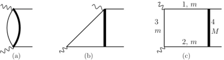
Fig. 1.(a)Two-loopnonplanardiagramcontributingtoNNLOmatchinginnonrelativisticfieldtheoryand(b)diagram obtainedfromitbycontractingthemassless-propagatorlines.AnadditionalmassMisintroducedtosimplifytheactual calculations(seediscussioninthetext).

offers the opportunity to considerably improve the accuracy of t -quark mass measurements at the CERN Large Hadron Collider and future linear colliders. As for NRQED applications, the best known one is probably the calculation of the parapositronium decay rate [83–87].

As already mentioned above, there are no new functions beyond polylogarithms at the one- loop level. So, the elliptic structures first appear at next-to-next-to-leading order (NNLO). One of the most complicated diagrams containing elliptic structure is the nonplanar one shown in Fig. 1(a). Applying integration-by-parts (IBP) identities [88,89], this diagram can be reduced to a sum of so-called master integrals with rational coefficients. When both massless lines are con- tracted, we obtain the diagram shown in Fig. 1(b) upon the replacement M = m. In this paper, we evaluate the latter diagram and all its subtopologies obtained by contracting some of its lines.

Moreover, as by a product, we even solve the more general problem with two different masses, as shown in Fig. 1(b).

Here and in the following, we work in dimensional regularization with d = 4 − 2ε space-time dimensions. In our previous paper [90], we presented the results for sunset diagrams obtained by contracting lines 1 and 2 in Fig. 1(b). The results of Ref. [90] were obtained up to and including the O(ε) terms and represented as fast converging series in the mass ratio x = m

²

/M

²

. The O (1) terms may also be found in Section 4.1. It is then easy to rewrite a given such series in terms of generalized hypergeometric functions

p

F

_p₋₁

[91], as

e

^2εγ^E

M

²

2ε+1

J

₀₁₀₂₂^mM

=

4

F

3

1 2

, 1, 1, 1

3 4

,

⁵₄

,

³₂

− x

²

4 + 1 4

d dδ

x

¹⁻^2δ

(1 − 2δ)

²

(1 − δ)(3 − 16δ)

⁴

F

₃

1, 1 − δ,

³₂

− δ,

³₂

− δ

5

4

− δ,

⁷₄

− δ, 2 − δ − x

²

4

δ=0

+ O (ε) ,

e

^2εγ^E

M

²

2ε

J

₀₁₀₁₂^mM

= − 1 2ε

²

− 1

2ε − 1

2 (1 + ζ

₂

) + x

4 (5 − 2 ln x) + x

²

9

⁴

F

3

1, 1, 1,

³₂

5 4

,

⁷₄

,

⁵₂

− x

²

4 − d dδ

x

³⁻^δ

(1 − δ)

²

(4 − δ)(15 − 46δ)

⁴

F

₃

1,

³₂

−

^δ₂

,

³₂

−

^δ₂

, 2 −

^δ₂

7

4

−

^δ₂

,

⁹₄

−

^δ₂

, 3 −

^δ₂

− x

²

4

δ=0

+ O (ε) ,

e

^2εγ^E

M

²

2ε−1

J

₀₁₀₁₁^mM

= − 1 ε

²

(1 + x

2 ) + 1

ε −3 + 1

4 ( −7 + 4 ln x)

− 7 − ζ

₂

+ x

8 5 − 4ζ

2

+ 8 ln x − 4 ln

²

x

− 2x

²

9

⁴

F

₃

1 2

, 1, 1, 1

5 4

,

⁷₄

,

⁵₂

− x

²

4

(4)

− 2 d dδ

x

³⁺^δ

(1 + δ)

²

(2 + δ)(4 + δ)(15 + 46δ)

⁴

F

₃

1, 1 +

₂^δ

,

³₂

+

₂^δ

,

³₂

+

₂^δ

7

4

+

^δ₂

,

⁹₄

+

^δ₂

, 3 +

^δ₂

− x

²

4

δ=0

+ O (ε) , (2) where ζ

_n

= ζ (n) denotes Riemann’s zeta function. A similar form was found for the Baxter Q function in Refs. [92,93]. Following our study in Ref. [90], it was shown in Ref. [94] that a similar hypergeometric representation is applicable for the considered sunset diagrams even without ε expansion. In the present paper, we extend the results of Ref. [90] for the case of three- and four-point diagrams (see Fig. 1) with O (1) accuracy.

This paper is organized as follows. In Section 2, we recall the central relation between the one- and two-loop diagrams, Eq. (3). Section 3 contains the details of the one-loop calculations.

In Section 4, we derive the series, integral, and hypergeometric representations of the considered two-loop diagrams in the general case of non-equal masses, M = m. Subsection 4.4 contains our results for the equal-mass case. Finally, in Section 5, we present our conclusions. In Appendix A, we explain the Frobenius solution for a system of differential equations.

2. Relation between one- and two-loop diagrams

As explained in Section 1, all two-loop Feynman diagrams considered in this paper have self-energy insertions built from two massive propagators as indicated in Fig. 1(b). These can be reduced to one-loop diagrams by representing the loop with the two massive propagators as an integral whose integrand contains a new propagator with a mass that depends on the variable of integration [20,21,32,33,90,95]. Graphically, this procedure has the following form:

= i

¹⁺^d

(a + b − d/2) (a) (b)

1 0

ds

s

^a⁺¹⁻^d/2

(1 − s)

^b⁺¹⁻^d/2

× , (3) where the loop involving the two propagators with mass square M

²

is replaced by one propagator with mass square M

₁²

/s + M

₂²

/(1 − s). The numbers a and b, indicating the powers of the scalar propagators, are called the propagator indices.

Equation (3) is easily derived from the Feynman parameter representation and was introduced in Euclidean and Minkowski spaces in Refs. [32,33] and [20,21], respectively. Here, we work in Minkowski space and thus follow Refs. [20,21].

As in Ref. [90], we adopt the following strategy. First, applying Eq. (3), we write expressions for the considered two-loop diagrams as integrals of one-loop diagrams involving propagators with masses that depend on the variable of integration. Next, in Section 3, we evaluate the one- loop integrals thus obtained and then, in Section 4, use these expressions to reconstruct the results for the two-loop diagrams involving two different masses with the help of Eq. (3). A similar strategy was also adopted for the calculation of certain four-loop tadpole diagrams in Ref. [95].

3. One-loop integrals

Let us consider the following one-loop box integral with two different masses, m and M, and

propagator indices a

1

, a

₂

, a

₃

, a

₄

:

(5)

Fig. 2.Typicalone-loopdiagramsresultingfromtheIBPreductionoftheintegralinEq. (4).Thethinandthicksolid linesrepresentscalarpropagatorswithmassesmandM,respectively.Inthecaseoftheboxdiagram(c),alsotheline numberingisindicated.

I

_a^mmmM

1a2a3a4

= I

_a^mM

1a2a3a4

= d

^d

l

π

^d/2

1 [ (l + q

₁

)

²

− m

²

]

^a¹

[ (l − q

₂

)

²

− m

²

]

^a²

[ l

²

− m

²

]

^a³

[ (l + q

₁

− p)

²

− M

²

]

^a⁴

, (4) where the kinematics in Eq. (1) is implied. Using IBP, the integral in Eq. (4) can always be reduced to a set of scalar master integrals with propagator indices 1 or 0. Some of these master integrals are shown in Fig. 2.

Following the line numbering in Fig. 2(c), the diagrams shown in Figs. 2(a)–(c) correspond to the integrals I

₀₀₁₁^mmmM

, I

₀₁₁₁^mmmM

, and I

₁₁₁₁^mmmM

, respectively. Notice that, in the course of the reduction, more master integrals appear: two bubbles, I

1000

and I

0001

, two more vertices, I

1110

and I

1101

, and one more self-energy, I

0110

. However, all these additional integrals only contain simple polylogarithmic structures, and their two-loop counterparts have no elliptic content. We omit these diagrams in our discussion, except for those that enter as subgraphs in the integrals I

₀₁₁₁^mmmM

and I

₁₁₁₁^mmmM

.

3.1. Two-point case

In the case of the two-point diagrams, IBP provides us with the relations I

₀₁₀₁^mM

(d − 3)

M

²

− 2m

²

= M

²

I

₀₀₀₂^M

− 2m

²

I

₀₀₂₀^m

− M

²

M

²

− 4m

²

I

₀₁₀₂^mM

, I

₀₀₁₁^mM

(d − 3)M

²

=

M

²

+ 2m

²

I

₀₀₀₂^M

− 2m

²

I

₀₀₂₀^m

− (4m

⁴

+ M

⁴

)I

₀₀₁₂^mM

, (5) which can be considered as the differential equations for the initial diagrams I

₀₁₀₁^mM

and I

₀₀₁₁^mM

, as

I

₀₁₀₂^mM

= d

dM

²

I

₀₁₀₁^mM

, I

₀₀₁₂^mM

= d

dM

²

I

₀₀₁₁^mM

. (6)

The integrals I

_000a^M

and I

_00a0^m

in Eq. (5) are tadpoles with masses M and m, respectively, I

_000a^M

= i( −1)

^a

(M

²

)

^a⁻^d/2

(a − d/2)

(a) , I

_00a0^m

= i( −1)

^a

(m

²

)

^a⁻^d/2

(a − d/2)

(a) . (7)

Similarly, using IBP and substituting m = 1 and d/dM

²

= − x

²

d/dx, we can deduce a differential equation for I

₁₂⁽¹⁾

= I

₀₁₀₂^mM

,

(1 − 2x)(1 − 4x) d

dx I

₁₂⁽¹⁾

− 4xI

₁₂⁽¹⁾

+ i(1 − 2x + 2x ln x) = 0 , (8)

(6)

which is valid up to O (ε) corrections. Equation (8) is easy to solve and, taking the boundary conditions at x = 0 into account, we have

M

²

i I

₁₂⁽¹⁾

= lnx

2x + (1 − 2x) 2x √

1 − 4x ln 1 + √ 1 − 4x 1 − √

1 − 4x + O (ε) , (9)

or, in terms of a series solution, M

²

i I

₁₂⁽¹⁾

= −1−

^∞

n=1

2n n

n

n + 1 x

ⁿ

ln x − 2S

1

(n − 1) + 2S

1

(2n − 1) − 1 n + 1

+O (ε) . (10) Now, IBP relations allow us to write down answers for the I

a⁽¹⁾₁a₂

integrals with other values of propagator indices. For example, we have

M

²

i I

₂₁⁽¹⁾

= − ln x

2x − 1

2x √

1 − 4x ln 1 + √ 1 − 4x 1 − √

1 − 4x + O (ε) , M

²

i I

₂₁⁽¹⁾

= 1 + lnx +

^∞

n=1

2n n

1 + 2n 1 + n x

ⁿ

× ln x + 2S

1

(2n − 1) − 2S

1

(n − 1) + 2

2n + 1 − 1 n + 1 − 1

n

+ O (ε) , e

^εγ^E

(M

²

)

^ε

i I

₁₁⁽¹⁾

= 1

ε + 2 + 1 − 2x 2x lnx +

√ 1 − 4x

2x ln 1 + √ 1 − 4x 1 − √

1 − 4x + O (ε) , e

^εγ^E

(M

²

)

^ε

i I

₁₁⁽¹⁾

= 1

ε + 1 +

^∞

n=1

2n n

x

ⁿ

1 + n

× ln x + 2S

1

(2n − 1) − 2S

1

(n − 1) − 1 n − 1

n + 1

+ O (ε) . (11) For m = M (x = 1), we have

M

²

i I

₁₂⁽¹⁾

= M

²

i I

₂₁⁽¹⁾

= − π 3 √

3 + O (ε) , e

^εγ^E

(M

²

)

^ε

i I

₁₁⁽¹⁾

= 1

ε + 2 − π

√ 3 + O (ε) . (12)

In the case of the integral I

₁₂⁽²⁾

= I

₀₀₁₂^mM

, the application of IBP relations leads to the following differential equation:

1 + 4x

²

d

dx I

₁₂⁽²⁾

+ 4xI

₁₂⁽²⁾

+ i(1 + 2x + 2x ln x) = 0 , (13) which is again valid up to O (ε) terms. The solution of Eq. (13) is straightforward and, taking the boundary conditions at x = 0 into account, yields

M

²

i I

₁₂⁽²⁾

= − 1

2x ln x + 1 4x √

1 + 4x

²

ln

√ 1 + 4x

²

− 1

√ 1 + 4x

²

+ 1 + ln

√ 1 + 4x

²

− 2x

√ 1 + 4x

²

+ 2x

+ O (ε) ,

(14)

(7)

or, in terms of a series solution, M

²

i I

₁₂⁽²⁾

= −1 −

∞ n=1

( −16x

²

)

ⁿ

(2n + 1)

2n n

+ 1 2x

∞ n=1

2n n

( − x

²

)

ⁿ

ln x + S

1

(2n − 1) − S

1

(n − 1) − 1 2n

+ O (ε) . (15)

The expressions for the I

_a⁽²⁾₁_a₂

integrals with other values of propagator indices can again be obtained with the help of IBP relations. For example, for I

₂₁⁽²⁾

and I

₁₁⁽²⁾

, we have

M

²

i I

₂₁⁽²⁾

= (2x − 1) M

²

i I

₁₂⁽²⁾

+ ln x + O (ε) , e

^εγ^E

(M

²

)

^ε

i I

₁₁⁽²⁾

= 1 ε +

1 + 4x

²

M

²

i I

₁₂⁽²⁾

+ 2(1 + x lnx) + O (ε) . (16) In the limit m = M (x = 1), we have

M

²

i I

₁₂⁽²⁾

= M

²

i I

₂₁⁽²⁾

= − 2

√ 5 ln 1 + √ 5

2 + O (ε) , e

^εγ^E

(M

²

)

^ε

i I

₁₁⁽²⁾

= 1

ε + 2 − 2 √

5 ln 1 + √ 5

2 + O (ε) . (17)

3.2. Three-point case

In the case of three-point diagrams, IBP yields the relation I

_011a^mM

= 1

2m

²

(a − 1)

(a − 1)I

001a

+ I

_002a₋₁

− (a − 1)I

010a

− I

_020a₋₁

, (18)

which, for example, allows us to obtain expressions for the integral I

₁₁₂⁽³⁾

= I

₀₁₁₂^mM

, (M

²

)

²

i I

₁₁₂⁽³⁾

= 1 2x √

1 − 4x ln 1 + √ 1 − 4x 1 − √

1 − 4x + 1

4x √ 1 + 4x

²

×

ln

√ 1 + 4x

²

− 1

√ 1 + 4x

²

+ 1 + ln

√ 1 + 4x

²

− 2x

√ 1 + 4x

²

+ 2x

+ O (ε) , (19)

or, in terms of a series solution, (M

²

)

²

i I

₁₁₂⁽³⁾

= −1 − 1 2x

∞ n=1

2n n

x

ⁿ

lnx + 2S

1

(2n − 1) − 2S

1

(n − 1) − 1 n

−

^∞

n=1

( − 16x

²

)

ⁿ

(2n + 1)

2n n

+ 1 2x

∞ n=1

2n n − x

²

n

× lnx + S

₁

(2n − 1) − S

₁

(n − 1) − 1 2n

+ O (ε) . (20)

(8)

To obtain an expression for the I

₁₁₁⁽³⁾

integral, we may consider the following, easy-to-obtain differential equation

³

:

d

dx I

₁₁₁⁽³⁾

+ 1

x(1 − 2x) I

₁₂⁽¹⁾

+ 1

x I

₁₂⁽²⁾

− i ln x

1 − 2x = 0 . (21)

The solution of Eq. (21), with account of the corresponding boundary conditions at x = 0,

⁴

is given by

M

²

i I

₁₁₁⁽³⁾

= 1 4x

ln

²

1 + √ 1 − 4x 1 − √

1 − 4x − 1 4 ln

²

√ 1 + 4x

²

− 1

√ 1 + 4x

²

+ 1 − 2I

1

(x)

+ O (ε) , (22) where

I

1

(x) = Li

2

( − R(x)) − Li

2

(R(x)) , R(x) = 1 − √ S(x) 1 + √

S(x) , S(x) =

√ 1 + 4x

²

− 2x

√ 1 + 4x

²

+ 2x . (23) In terms of a series, the solution takes form

M

²

i I

₁₁₁⁽³⁾

= 1 + ln x +

^∞

n=1

( − 16x

²

)

ⁿ

(1 + 2n)

²

2n n

+

^∞

n=1

2n n

(1 + 2n) (1 + n)

²

x

ⁿ

× lnx + 2S

1

(2n − 1) − 2S

1

(n − 1) + 2

2n + 1 − 2 n + 1 − 1

n

+ 1 4x

∞ n=1

2n n

− x

²

n

n 1

n + S

₁

(n − 1) − S

₁

(2n − 1) − ln x

+ O (ε) . (24) In the limit m = M (x = 1), we have

M

²

i I

₁₁₁⁽³⁾

= 1 2 Li

2

√ 5 − 1

2 − 1 2 Li

2

1 − √

5 2

− 1 16 ln

²

√ 5 + 1

√ 5 − 1 − π

²

9 + O (ε) , (M

²

)

²

i I

₁₁₂⁽³⁾

= π 3 √

3 − 2

√ 5 ln 1 + √ 5

2 + O (ε) . (25)

3.3. Four-point case

The solution of the four-point case is simple. In this case, we may exploit the fact that the propagators of the integral I

_a^mM₁_a₂_a₃_a₄

in Eq. (4) are linearly dependent in the special kinematics of Eq. (1), so that diagrams with four propagators are reduced to ones with at least one propagator less. Namely, we have the relation

1 = (l + q

₁

)

²

+ (l − q

₂

)

²

− 2(l + q

₁

− p)

²

+ 2(M

²

− m

²

)

2M

²

, (26)

which can be used to obtain the following expressions:

3 Asbefore,thisfollowsfromIBPrelationsandisvaliduptoO(ε)terms.

4 InthelimitM²→ ∞,theintegralI₁₁₁⁽³⁾goestozero.

(9)

I

₁₁₁₁^mM

= 1 M

²

I

₀₁₁₁^mM

− I

₁₁₁₀^mM

= 1

M

²

I

₁₁₁⁽³⁾

− I

₁₁₁₀^mM

, I

₁₁₁₂^mM

= 1

M

²

I

₀₁₁₂^mM

− 1

M

²

I

₀₁₁₁^mM

+ 1 M

²

I

₁₁₁₀^mM

= 1 M

²

I

₁₁₂⁽³⁾

− 1

M

²

I

₁₁₁⁽³⁾

+ 1 M

²

I

₁₁₁₀^mM

, (27) where

m

²

i I

₁₁₁₀^mM

= − π

²

8 + O (ε) . (28)

4. Two-loop diagrams

We are now ready to evaluate the two-loop diagrams J

_010a^mM

1a₂

, J

_011a^mM

1a₂

, and J

_111a^mM

1a₂

, which can be obtained from J

_b^mM

1b2b3a1a2

shown in Fig. 1(b). The latter integral has the expression J

_b^mM

1b₂b₃a₁a₂

=

d

^d

k d

^d

k

₁

π

^d

1 (k

²

− m

²

)

^b³

[ (k + q

₁

)

²

− m

²

]

^b¹

[ (k − q

₂

)

²

− m

²

]

^b²

× 1

[ (k

₁

+ q

₁

/2 − q

₂

/2)

²

− M

²

]

^a¹

[ (k

₁

− k)

²

+ M

²

]

^a²

, (29) where again the special kinematics of Eq. (1) is implied. Exploiting the rule of Eq. (3), we replace the k

1

integration in Eq. (29) with the integration over the variable s from the corresponding one-loop integral I

_...a^mM

with the replacement M

²

→ μ

²

= M

²

/ [ s(1 − s) ]. Indeed, calling the above two-loop integral J

_...a^mM

1a₂

and the corresponding one-loop diagram I

_...a^mM

, we have J

_...a^mM

1a2

= (a)

(a

1

)(a

2

)

1 0

dss

^a^˜¹⁻¹

(1 − s)

^a^˜²⁻¹

I

_...a^mμ

, (30) where a ˜

_i

= d/2 − a

_i

and a = a

₁

+ a

₂

− d/2. We note that, strictly speaking, in Eq. (30), we should use the one-loop integrals I

_...,k^mM₊_ε

, where k = 0, 1, 2. On the other hand, in Section 3, we presented results for the I

_...k^mM

integrals with O (1) accuracy only. However, the latter are sufficient to determine the most complicated contributions from the two-loop diagrams, containing series in n. The less complicated terms can be obtained directly from the two-loop diagrams, either by using asymptotic expansions or differential equations. Moreover, the knowledge of the Frobenius solutions of the differential equations together with the ansätze for the occurring sums is sufficient to determine the required expressions for the two-loop diagrams (see Appendix A).

4.1. Series representations

Let us start with the two-point sunset diagrams. It is known, e.g. from Ref. [96], that for the special kinematics in Eq. (1) there exist three master integrals. Choosing the latter to be J

₀₁₀₁₁^mM

, J

₀₁₀₁₂^mM

, and J

₀₁₀₂₂^mM

and following the above general procedure, we obtain after some calculations

e

^2εγ^E

M

²

2ε+1

J

₀₁₀₂₂^mM

= J

₁₂₂⁽¹⁾

+ J

₁₂₂⁽²⁾

+ O (ε) , e

^2εγ^E

M

²

2ε

J

₀₁₀₁₂^mM

= − 1 2

1 ε

²

+ 1

ε + 1 + ζ

₂

+ J

₁₁₂⁽¹⁾

+ J

₁₁₂⁽²⁾

+ O (ε) ,

(10)

e

^2εγ^E

M

²

2ε−1

J

₀₁₀₁₁^mM

= − 1

ε

²

+ 3

ε + 7 + ζ

₂

+ x − 1 2

1 ε

²

+ 7

2ε − 5 4 + ζ

₂

+

1 ε + 1

ln x − 1

2 ln

²

x

+ J

₁₁₁⁽¹⁾

+ J

₁₁₁⁽²⁾

+ O (ε) , (31) where

J

₁₂₂⁽¹⁾

= 1 2x

∞ n=1

2n n

4n

2n

− x

²

n

n 1

2n + S

1

− 3S

1

+ 2S

1

− ln x

,

J

₁₂₂⁽²⁾

= 1 4x

²

∞ n=1

−16x

²

n

2n n

4n 2n

1 − 4n n

²

(2n − 1) ,

J

₁₁₂⁽¹⁾

= x

4 (5 − 2 ln x) + x

2

∞ n=1

2n n

4n

2n

− x

²

n

(n + 1)(4n + 1) 1

2(n + 1) + 2

1 + 4n + S

1

− 3S

1

+ 2S

1

− lnx

,

J

₁₁₂⁽²⁾

= − 1 4

∞ n=1

−16x

²

n

2n n

4n 2n

1 n

²

(2n + 1) ,

J

₁₁₁⁽¹⁾

= x 2

∞ n=1

2n n

4n

2n

− x

²

n

n(n + 1)(4n + 1)

×

ln x − S

₁

+ 3S

1

− 2S

1

− 1

2n − 1

2(n + 1) − 2 1 + 4n

, J

₁₁₁⁽²⁾

= 1

2

∞ n=1

−16x

²

n

2n n

4n 2n

1 n

²

(2n − 1)(2n + 1) . (32)

Here, for brevity, we have omitted the arguments of the harmonic sums S

1

(n) and introduced the short-hand notations

S

₁

= S

₁

(n − 1) , S

₁

= S

₁

(2n − 1) , S

₁

= S

₁

(4n − 1) . (33)

For the practical applications mentioned in Section 1, we also need the O (ε) terms of the sun-

set diagrams. We do not present them here for a general value of x, since the corresponding

expressions are too lengthy. However, they may be found in Ref. [90].

(11)

Similarly, for the three- and four-point two-loop integrals, we have

⁵

e

^2εγ^E

M

²

2ε+1

J

₀₁₁₁₂^mM

= − 1 2 + 1

x Li

3

(x) − 1

2 ln x Li

2

(x)

+ J

₁₁₁₂⁽¹⁾

+ J

₁₁₁₂⁽²⁾

+ O (ε) , e

^2εγ^E

M

²

2ε

J

₀₁₁₁₁^mM

= − 1 2ε

²

+ 1

ε

lnx − 1 2

− 3 2 − ζ

₂

2 + [2 − ln(1 − x) ] ln x − ln

²

x

2 − Li

2

(x) + 1

x {2 Li

3

(x) + Li

2

(x) + lnx [ln(1 − x) − Li

2

(x)]}

+ J

₁₁₁₁⁽¹⁾

+ J

₁₁₁₁⁽²⁾

+ O (ε) , e

^2εγ^E

M

²

2ε+2

J

₁₁₁₁₂^mM

= 1 2x

^3/2

Li

2

− √ x

− Li

2

√ x + 1

2 ln x ln 1 + √ x 1 − √

x

+ 1

4x {3 + Li

2

(x) + lnx [ln(1 − x) − 2] } + J

₁₁₁₁₂⁽¹⁾

+ J

₁₁₁₁₂⁽²⁾

+ O (ε) ,

e

^2εγ^E

M

²

2ε+1

J

₁₁₁₁₁^mM

= 1 x

^3/2

2 Li

2

− √ x

− 2 Li

2

√ x

+ ln x ln 1 + √ x 1 − √

x

+ 1 x

1 2ε + 4 − Li

3

(x) + Li

2

(x) + ln x 1

2 Li

2

(x) + ln(1 − x) − 5 2

+ J

₁₁₁₁₁⁽¹⁾

+ J

₁₁₁₁₁⁽²⁾

+ O (ε) , (34)

where

J

₁₁₁₂⁽¹⁾

= 1 8x

∞ n=1

− x

²

n

2n n

4n

2n 1

n

²

lnx − 1

n − S

₁

+ 3S

1

− 2S

1

,

J

₁₁₁₂⁽²⁾

= − 1 2

∞ n=1

−16x

²

n

2n n

4n 2n

1 (2n + 1)

²

(4n + 1) ,

J

₁₁₁₁⁽¹⁾

= 1 4x

∞ n=1

2n n

4n

2n

− x

²

n

²

(2n − 1) 1

n + 1

2n − 1 + S

₁

− 3S

1

+ 2S

1

− ln x

,

J

₁₁₁₁⁽²⁾

= 1 2

∞ n=1

− 16x

²

n

2n n

4n 2n

1 n(2n + 1)

²

(4n + 1) ,

5 Here,wehavesummedseriescorrespondingtomultiplepolylogarithms.

(12)

J

₁₁₁₁₂⁽¹⁾

= 1 8x

∞ n=1

− x

²

n

2n n

4n

2n

1 n(4n + 1)

lnx − 1 2n − 2

4n + 1 − S

₁

+ 3S

1

− 2S

1

,

J

₁₁₁₁₂⁽²⁾

= 1 16x

²

∞ n=1

−16x

²

n

2n n

4n 2n

1 n

²

(2n − 1) ,

J

₁₁₁₁₁⁽¹⁾

= 1 8x

∞ n=1

− x

²

n

2n n

4n

2n

1 n

²

(4n + 1)

1 n + 2

4n + 1 + S

1

− 3S

1

+ 2S

1

− lnx

,

J

₁₁₁₁₁⁽²⁾

= 1 8x

²

∞ n=1

−16x

²

n

2n n

4n 2n

1 n

²

(2n − 1)

²

. (35)

4.2. Integral representations

Although the series expansions obtained in Subsection 4.1 are rapidly converging, it is useful to also find integral representations for the considered diagrams. To derive integral representations, it is helpful to rewrite the above series representations in the following form:

J

₁₂₂⁽²⁾

= − 1 8x

²

∞ n=1

− 16x

²

n

²

(n)(2n − 1) (4n − 1) , J

₁₁₂⁽²⁾

= − 1

4

∞ n=1

−16x

²

n

²

(n)(2n + 1) (4n + 1)

1 2n + 1 , J

₁₁₁⁽²⁾

=

^∞

n=1

−16x

²

n

(n)(n + 1)(2n − 1) (4n + 1)

1 2n + 1 , J

₁₁₁₂⁽²⁾

= 1

16x

²

∞ n=1

−16x

²

n

²

(n)(2n − 1) (4n − 1)

1 2n − 1 , J

₁₁₁₁⁽²⁾

= −

^∞

n=1

−16x

²

n

(n)(n + 1)(2n + 1) (4n + 3)

1 2n + 1 , J

₁₁₁₁₂⁽²⁾

= 1

8x

²

∞ n=1

−16x

²

n

(n)(n + 1)(2n − 1) (4n + 1) , J

₁₁₁₁₁⁽²⁾

= − 1

4x

²

∞ n=1

−16x

²

n

(n))(n + 1)(2n − 1) (4n + 1)

1 2n − 1 . (36)

Now, we write J

_1....⁽¹⁾

= d

dδ J

_1....⁽¹⁾

(δ)

δ=0

, (37)

(13)

where

J

₁₂₂⁽¹⁾

(δ) = 1 x

∞ n=1

− x

²

n

x

⁻^δ

²

(2n + 1 − δ)(2n − δ)

²

(n + 1 − δ/2)(4n + 1 − 2δ) , J

₁₁₂⁽¹⁾

(δ) = x

2

∞ n=0

− x

²

_n

x

⁻^δ

³

(2n + 1 − δ)

(n + 1 − δ/2)(n + 2 − δ/2)(4n + 2 − 2δ) , J

₁₁₁⁽¹⁾

(δ) = − x

∞ n=1

− x

²

n

x

⁻^δ

²

(2n + 1 − δ)(2n − δ)

(n + 1 − δ/2)(n + 2 − δ/2)(4n + 2 − 2δ) , J

₁₁₁₂⁽¹⁾

(δ) = − 1

2x

∞ n=1

− x

²

n

x

⁻^δ

(2n + 1 − δ)

²

(2n − δ)

²

(n + 1 − δ/2)(4n + 1 − 2δ) , J

₁₁₁₁⁽¹⁾

(δ) = 1

x

∞ n=1

− x

²

n

x

⁻^δ

(2n + 1 − δ)(2n − δ)(2n − 1 − δ)

²

(n + 1 − δ/2)(4n + 1 − 2δ) , J

₁₁₁₁₂⁽¹⁾

(δ) = − 1

4x

∞ n=1

− x

²

n

x

⁻^δ

²

(2n + 1 − δ)(2n − δ)

²

(n + 1 − δ/2)(4n + 1 − 2δ) , J

₁₁₁₁₁⁽¹⁾

(δ) = 1

2x

∞ n=1

− x

²

n

x

⁻^δ

(2n + 1 − δ)

²

(2n − δ)

²

(n + 1 − δ/2)(4n + 2 − 2δ) . (38) Starting from this point, the corresponding integral representations can be obtained in two steps.

First, we rewrite the functions (4n + 2a(n, δ)), with some a(n, δ) depending on the series under consideration, in the denominators as products of two functions, (2n + a(n, δ)) and (2n + a(n, δ) + 1/2). Second, we represent the ratio of the function (2n + b(n, δ)), with some b(n, δ) depending on the series under consideration, in the numerator and the function (2n + a(n, δ) + 1/2) in the denominator as

(2n + b(n, δ)) (2n + a(n, δ) + 1/2) =

1 0

dt t

²ⁿ⁺^b(n,δ)⁻¹

(1 − t )

^a(n,δ)⁻^b(n,δ)⁻^1/2

a(n, δ) − b(n, δ) + 1/2 . (39) The remaining series can now be summed, and we are left with the sought integral representations over t. This way, we obtain the following integral representations for the two-point diagrams:

J

₁₂₂⁽¹⁾

= − 1 2x

1 0

dt t √

1 − t

√ 1

1 + 4A

²

L

₁

(A) − 2 ln A

, (40)

J

₁₂₂⁽²⁾

= − 1 2x

1 0

dt t √

1 − t

√ 1

1 + 4A

²

L

₂

(A) , (41)

J

₁₁₂⁽¹⁾

= − 1 x

1 0

dt t

²

√

1 − t

1 + 4A

²

L

₁

(A) − 2 ln A

, (42)

(14)

J

₁₁₂⁽²⁾

= − 1 x

1

0

dt t

²

√

1 − t

1 + 4A

²

L

₂

(A) + 4A

, (43)

J

₁₁₁⁽¹⁾

= 4 x

1 0

dt

√ 1 − t t

³

1 + 4A

²

L

1

(A) − 2 ln A + 2A

²

− 4A

²

lnA

, (44)

J

₁₁₁⁽²⁾

= 4 x

1 0

dt

√ 1 − t t

³

1 + 4A

²

L

2

(A) + 4A

, (45)

where A = xt/4, L

₁

(A) = ln

√ 1 + 4A

²

− 1

√ 1 + 4A

²

+ 1 , L

₂

(A) = ln

√ 1 + 4A

²

− 2A

√ 1 + 4A

²

+ 2A . (46) Notice that the above integral representations for the sunset diagrams are simpler than those in Ref. [90], which involved some dilogarithms. Similarly, for the functions entering the expressions for the three- and four-point integrals, we have

J

₁₁₁₂⁽¹⁾

= − 1 4x

1 0

dt t √

1 − t ln

²

A − 1 4 L

₁

(A)

²

,

J

₁₁₁₂⁽²⁾

= 1 2x

1 0

dt t √

1 − t [I

1

(A) + 2A] ,

J

₁₁₁₁⁽¹⁾

= 1 x

1 0

dt

√ 1 − t

t

²

ln

²

A − 1 4 L

₁

(A)

²

,

J

₁₁₁₁⁽²⁾

= − 2 x

1 0

dt

√ 1 − t

t

²

[I

1

(A) − 1 + 2A] ,

J

₁₁₁₁₂⁽¹⁾

= 1 8x

1 0

dt

√ 1 − t t

√ 1

1 + 4A

²

L

₁

(A) − 2 ln A

,

J

₁₁₁₁₂⁽²⁾

= 1 8x

1 0

dt

√ 1 − t t

√ 1

1 + 4A

²

L

2

(A) ,

J

₁₁₁₁₁⁽¹⁾

= 1 4x

1 0

dt

√ 1 − t

t ln

²

A − 1 4 L

₁

(A)

²

,

J

₁₁₁₁₁⁽²⁾

= − 1 2x

1 0

dt

√ 1 − t

t I

₁

(A) , (47)

(15)

where I

₁

(A) is defined in Eq. (23). Such correspondence reveals a deep relation between the subintegral expressions of the two-loop integrals and the corresponding one-loop results, in agreement with the general prescription in Eq. (30).

To check that the above integral representations are simplest, it is convenient to use the following relations between the functions J

_...12⁽ⁱ⁾

and J

_...11⁽ⁱ⁾

(i = 1, 2):

d dx

1 x J

₁₁₁⁽ⁱ⁾

= − 2

x

²

J

₁₁₂⁽ⁱ⁾

− δ

₁ⁱ

1 4 x(5 − 2 ln x)

, (48)

x d

dx J

₁₁₁₁⁽ⁱ⁾

= −2J

₁₁₂⁽ⁱ⁾

+ δ

₂ⁱ

, (49) d

dx

x J

₁₁₁₁₁⁽ⁱ⁾

= − 2J

₁₁₁₁₂⁽ⁱ⁾

, (50)

where δ

ⁱ₂

is the Kronecker symbol, which directly follow from the corresponding series representations.

Indeed, in the simplest forms of the integral representations, these relations can easily be reproduced. As a first example, let us consider Eq. (48) with i = 2. From Eq. (45), we have

d dx

1 x J

₁₁₁⁽²⁾

= d dx

1 0

dt

√ 1 − t t

1 4A

²

1 + 4A

²

L

₂

(A) + 4A

=

1 0

dt

√ 1 − t t

d dx

1 4A

²

1 + 4A

²

L

₂

(A) + 4A

. (51)

Now, notice that the expression in brackets on the r.h.s. of Eq. (51) only depends on A. So, we can replace the derivative with respect to x acting on it with

d dx = dA

dx d dA = t

2 d

dA . (52)

Similarly, we have d

dt = dA dt

d dA = x

2 d

dA , (53)

so that, on the r.h.s. of Eq. (51), we can make the replacement d

dx = t x

d

dt , (54)

that is d dx

1 x J

₁₁₁⁽²⁾

=

1 0

dt

√ 1 − t x

d dt

1 4A

²

1 + 4A

²

L

₂

(A) + 4A

. (55)

Next, using IBP, we have d

dx 1

x J

₁₁₁⁽²⁾

= 1 x

√

1 − t 1 4A

²

1 + 4A

²

L

2

(A) + 4A

^t=1

t=0

−

1 0

dt d

dt

√ 1 − t 1

4A

²

1 + 4A

²

L

₂

(A) + 4A ⎫

⎬

⎭ . (56)

(16)

The first term on the r.h.s. of Eq. (56) is equal to zero, and d

dt

√ 1 − t = − 1 2 √

1 − t . (57)

So, finally, we have d

dx 1

x J

₁₁₁⁽²⁾

= 1 2x

1 0

√ dt 1 − t

1 4A

²

1 + 4A

²

L

₂

(A) + 4A

= 2 x

³

1 0

dt t

²

√

1 − t

1 + 4A

²

L

₂

(A) + 4A

= − 2 1

x

²

J

₁₁₂⁽²⁾

, (58)

where we have used Eq. (43) in the third equality. We thus observe that Eq. (48) with i = 2 is correct.

As a second example, let us consider Eq. (48) with i = 1. Repeating steps similar to those in Eqs. (51)–(58), we have

d dx

1 x J

₁₁₁⁽¹⁾

= 2 x

³

1 0

dt t

²

√

1 − t

1 + 4A

²

L

₁

(A) − 2 ln A + 2A

²

− 4A

²

lnA

. (59)

Then, the evaluation of the terms proportional to A

²

on the r.h.s. of Eq. (59) gives 1

4x

1 0

√ dt

1 − t (1 − 2 ln A) = 1

2x (5 − 2 ln x) , (60)

so that, finally, we have d

dx 1

x J

₁₁₁⁽¹⁾

= 2 x

³

⎧ ⎨

⎩

1 0

dt t

²

√

1 − t

1 + 4A

²

L

1

(A) − 2 ln A + x

²

4 (5 − 2 ln(x)

⎫ ⎬

⎭

= −2 1 x

²

J

₁₁₂⁽¹⁾

− x

4 (5 − 2 ln x)

, (61)

where we have used Eq. (42) in the second equality. We thus observe that Eq. (48) with i = 1 is also correct.

4.3. Representations in terms of generalized hypergeometric functions

For the two-point sunset-type diagrams, the results in terms of hypergeometric functions were

already given in Eq. (2). So, here we present such results for the three- and four-point diagrams

only. The series representations obtained in Subsection 4.1 can be readily expressed in terms of

hypergeometric functions and their derivatives. We thus obtain