Weaning of Mechanically Ventilated Patients in the Intensive Care Unit: A Clinician-in-the-Loop Reinforcement Learning Approach

(1)

Research Collection

Bachelor Thesis

Weaning of Mechanically Ventilated Patients in the Intensive Care Unit: A Clinician-in-the-Loop Reinforcement Learning Approach

Author(s):

Rüegsegger, Nicola Elias Publication Date:

2021

Permanent Link:

https://doi.org/10.3929/ethz-b-000473932

Rights / License:

In Copyright - Non-Commercial Use Permitted

This page was generated automatically upon download from the ETH Zurich Research Collection. For more information please consult the Terms of use.

(2)

Weaning of Mechanically Ventilated Patients in the Intensive Care Unit:

A Clinician-in-the-Loop

Reinforcement Learning Approach

Bachelor Thesis Nicola Elias R¨ uegsegger

January 30, 2021

Advisors: Matthias Hüser, Olga Mineeva Supervisor: Prof. Dr. Gunnar Rätsch Department of Computer Science, ETH Zürich

(3)

(4)

Abstract

The COVID-19 pandemic has strained intensive care unit (ICU) resources globally and especially mechanical ventilation has become a bottleneck. While there are established clinical guidelines and best practices on the management and weaning procedure of mechanically ventilated patients, the rich data sets collected at ICUs provide the possibility to deploy machine learning techniques with the potential to improve current clinical practice. Thereby, the goal should be twofold, providing the best patient care while keeping ventilation times as short as possible. Since weaning is essentially a sequential decision making process, reinforcement learning is an especially well suited approach for the creation of novel intelligent clinical recommendation systems.

Traditionally, a reinforcement learning algorithm learns to take the best possible action at every time step. However, in medical practice there is often additional information available to clinicians, e.g. a newly dis- covered intolerance to a given medication, with the possibility to ren- der a recommendation made by a learning algorithm irrelevant. For an intelligent system to be useful in the clinical setting, it is therefore important that additional information available to the clinician can be incorporated in the decision making process. This is the approach of novel clinician-in-the-loop reinforcement learning algorithms based on near-optimal set-valued policies which give clinicians a selection of possible actions to be taken. The following thesis implements such a reinforcement learning algorithm for the first time in the setting of weaning mechanically ventilated patients. In our implementation and for our data set, the algorithm is able to find an average of up to 1.7 near-optimal actions for each patient state. At the same time, it scores an average reward of 39 on the test set with a 1h sampling rate, com- parable to Q-learning (33) and value iteration (28) and outperforming the empirically estimated policy derived from the data set (-45) as well as naive policy implementations (-99 to -6). Near-optimal set-valued policies are therefore a promising class of algorithms in the setting of weaning mechanically ventilated patients. Thereby, they have the potential to shorten ventilation periods and improve medical outcomes while at the same time giving clinicians the possibility to incorporate additional knowledge into the decision making process.

(5)

(6)

Acknowledgements

I would like to thank my supervisor, Prof. Dr. Gunnar R¨atsch, for giving me the opportunity to write this thesis at the Biomedical Informatics group, thereby allowing me to combine my enthusiasm for reinforcement learning with my medical background. Also, I would like to express my sincere gratitude to my two advisors, Matthias H ¨user and Olga Mineeva. Not only did they share their vast knowledge with me, they were beyond support- ive, guiding me every step along the way of this exciting thesis. I am also thankful to Dr. med. Martin Faltys for his valuable advice on how to best approximate a patient’s sedation level in the ICU. Finally, I would like to thank my family and friends for their loving support during the development of this thesis.

(7)

(8)

Chapter 1 Introduction

Managing mechanically ventilated patients can be highly challenging. Not only are patients often terminally ill, there is currently a lack of high level evidence to guide treatment decisions—it has been estimated that only around 9% of treatment recommendations in critical care are based on grade A evidence [1]. In most recent times, the coronavirus pandemic put en enor- mous additional pressure on ICUs, leading to ventilator shortages around the globe [2]. While clinical outcomes with prolonged mechanical ventilation haven been known to be often very poor [3], COVID-19 made finding the earliest possible point in time to extubate a patient, and therefore freeing up highly scarce resources for other patients, even more urgent.

Due to the vast amount of data collected in intensive care, machine learning approaches pose the potential to improve current clinical practices and help with clinical decision making where other sources of evidence may be absent. Since patient care is inherently a sequential decision making process, reinforcement learning is an especially well suited approach and has therefore gained significant attention in the machine learning research com- munity over the recent years. Applications have included finding optimal medication doses, medication choices, individual target lab values and tim- ings of interventions, including ventilator weaning [4].

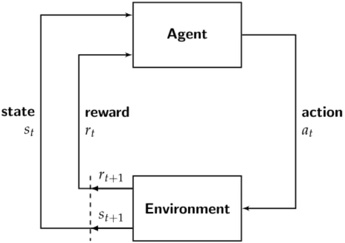
In reinforcement learning, an agentinteracts with its environment. At every point int time, the environment is in a certain state. Every time the agent takes an action, the environment returns a new state plus a reward [5]. In a healthcare setting, the environment is typically the patient, the states are values of variables defining the patients health status, actions are a therapeutic intervention and finally the reward is some measure of a clinical objective following the intervention [4]. During training on medical data, an agent learns which actions to take for every observable state in order to maximize the expected reward. While this approach allows to find optimal actions, it has one major drawback in the healthcare setting: Recommend-

(11)

1. Introduction

ing a single action for a given state does not allow the clinician to consider personal experience or additional information not known to the learning system. Even from a strictly mathematical perspective recommending only one action might not be desirable. Consider the situation where a range of actions all yield almost exactly the same outcome, the difference being much smaller than the variance expected with the given data set. Now choosing the best action resembles choosing a random action.

In this thesis, we implement a novel approach to reinforcement learning, near-optimal set-valued policies(NOSVP), first demonstrated with clinical data in 2020 [6]. Its novelty lies in a simple adaption to the classical reinforcement learning algorithmQ-learning: Instead of learning an optimal action for a given state, a chosen parameterζ allows the algorithm to relax the optimality condition, thereby potentially learning a set of near-optimal actions for each state. Consequently, this approach yields a new trade-off between the number of recommendations per state and the overall performance of the algorithm. However, if carefully designed, the NOSVP algorithm has the potential to give clinicians a choice of different actions, allowing them to incorporate additional knowledge or personal experience into the decision making process. In this thesis we evaluate the NOSVP algorithm for the objective of finding intelligent treatment recommendations in the weaning process of mechanically ventilated patients.

This report is structured into a total of six different chapters. After this introduction, we look at the medical process of weaning mechanically ventilated patients, explain the most important concepts in reinforcement learning and explore related work. Then, in chapter 3, we detail all the methods applied in this thesis, starting with the critical care data set and MDP definition and ending with the evaluation metrics used to create the results in chapter 4.

In chapter 5 we then discuss our obtained results before concluding our research in chapter 6.

Finally, a few notes on the foundations and implementation of this thesis.

Our research builds on previous reinforcement learning studies with the objective of ventilator weaning published in the years 2017 - 2020 [7, 8, 9] as well as on the 2020 publication of the NOSVP algorithm [6] and the publicly available corresponding code base [10] which we adapted and extended for our data set and objective. The implementation of this thesis can be found on Github(currently only accessible within the research group at ETH Z ¨urich).

The code is structured in a way that allows for the command line submission of the entire extraction-preprocessing-learning pipeline to the ethsec / Leon- hard cluster environment. Where possible within the scope of this thesis, the implementation is parallelized in order to best use the multiprocessor setup.

(12)

Chapter 2 Background

This chapter lays the foundations for the following chapters in three key areas important to this thesis: the management of mechanically ventilated patients, the fundamentals of reinforcement learning and relevant previous machine learning research. Our own work then follows in chapter 3 and our results are presented in chapter 4.

2.1 Weaning of mechanically ventilated patients

Weaningdescribes the entire process of liberating a patient from mechanical ventilation and from the endotracheal tube [11]. An estimated 40% of the time spent on a ventilator is dedicated to the weaning process [12]. Both, premature and delayed weaning, are known to lead to adverse effects [13].

Thereby, delayed weaning may lead to complications including:

• Ventilator induced lung injury

• Ventilator associated pneumonia

• Ventilator induced diaphragmatic dysfunction

Premature weaning, on the other hand, may lead to complications including:

• Loss of the airway

• Defective gas exchange

• Aspiration

• Respiratory muscle fatigue

Event though there is a large range of weaning criteria helping clinicians in the decision making process, the best course of action often remains unknown [13]. Consequently, finding the right point in time to wean a patient

(13)

2. Background

is both important and nontrivial. It has been shown that using clear weaning protocols leads to shorter durations of mechanical ventilation [14]. The same is true for automated approaches whereby ventilators automatically adjust the mechanical ventilation support given to a patient [15]. However, there is a large heterogeneity both in terms of protocols and ventilators used, rendering clinical studies and clear recommendations more difficult [13].

Analogously to previous reinforcement learning research aiming at improv- ing the weaning process [7, 8, 9], in this thesis we focus exclusively on two sets of actions taken by clinicians, adjusting the sedation level and either keeping a patient on the ventilator or extubating them.

2.2 Reinforcement learning

In this section, we give an overview of the most important concepts inrein- forcement learning, an area ofmachine learning. The actual algorithms used in this thesis are then introduced in chapter 3.

Richard Sutton and Andrew Barto define reinforcement learning in their seminal bookReinforcement Learning: An Introduction first published in 1998 as [5]:

Reinforcement learning is about learning from interaction how to behave in order to achieve a goal.

Essentially, reinforcement learning is about finding the best course of actions by trial and error, thereby learning from experience on how to behave in order to maximize the chance for a desired reward. This is in contrast to two other popular branches of machine learning,supervised learningandunsuper- vised learning. Both of which have a classification objective, e.g. recognizing sounds or classifying images.

2.2.1 Finite Markov decision process

In reinforcement learning, the finiteMarkov decision process(MDP) defines a framework for an agent interacting with its environment over a sequence of discrete time steps with the following components [5]:

• A finite state space S

• A finite action spaceA

• A finite reward space R

• A transition function p:R × S × S × A →[0, 1]

At every time step t, the environment is in a statest ∈ S. The agent then takes an actiona_t∈ A, thereby changing the state of the environment which

(14)

2.2. Reinforcement learning returns a new state s_t+1 ∈ S plus a rewardr_t+1 ∈ R. See Figure 2.1 for a

graphical representation of the agent-environment interactions in an MDP, as adapted from Sutton and Barto [5].

Agent

Environment

action at

reward rt

state st

rt+1

st+1

Figure 2.1: Markov decision process

In an MDP, a states_t ∈ Shas to incorporate all knowledge about past agent- environment interactions which could make a difference for the future. Or in other words, it is enough for the agent to just see the current state in order to decide on the best action to take, no information about the past is needed.

This is called theMarkov property.

The transition function p defines the behavior of the environment, i.e. the probability that the environment returns a specific reward-state pair (r ∈ R, s⁰ ∈ S) for an action a ∈ A in a state s ∈ S: p(r,s⁰|s,a). Often, the transition function is unknown and the environment treated as a black box.

Corresponding reinforcement learning algorithms are calledmodel-free, since they do not assume a model of the environment. Conversely, algorithms with knowledge of the transition function are called model-based. In this thesis we implement and evaluate algorithms for both classes.

2.2.2 Value functions Q and V

During the interactions with the environment and with the received rewards, an agent learns about the expected long term values for states and for state- action pairs, leading to the twovalue functions, thestate value function V and the action value function Q. E.g. V(s)represents the expected value of state s ∈ S, considering all possible next actions and next states an agent would take and encounter.

(15)

2. Background 2.2.3 Policy

Ultimately, an agent wants to learn how to behave in each state in order to receive the highest cumulative reward possible. This learned behavior is the policy π: For each state s ∈ S, π(s) returns the action(s) the agent would take. Often, the policy is built in a greedy fashion, choosing in each state s ∈ S an action a ∈ A such that Q(s,a)is maximized. However, V and Q also depend on the policy. The expected cumulative reward of a state or a state-action pair depends on how the agent will behave in the future, i.e.

what other states and actions will follow. Therefore, V and Q are always policy specific and often also written Vπ and Qπ. This interdependence between the value functions and the policy leads to the two core update steps taught in classical reinforcement learning: the policy gets updated using the newest values of the value function (policy improvement), then the value function gets updated with the newest policy (policy evaluation) [5].

However, current reinforcement learning algorithms usually do not make such an explicit distinction between the two steps and often perform both at the same time. A policy can either be deterministic, i.e. returning exactly one action per state, or probabilistic with a probability distribution over the action spaceA. Strictly speaking, also the deterministic policy is an instance of the probabilistic one—the probability of one action is set to 1, while the others are set to 0.

In this thesis we build policies with several different approaches. Their implementations are detailed in chapter 3 and then their performances eval- uated and compared in chapter 4.

2.3 Related work

While there has been a range of reinforcement learning research focusing on critical care [4] and several machine learning approaches to improve the weaning process in particular [16], a few of the most recent ones directly serve as the scientific foundation for this thesis. We present and briefly summarize each of them in this section.

In 2017, Prasad et al. publishedA Reinforcement Learning Approach to Weaning of Mechanical Ventilation in Intensive Care Units[7], a paper evaluating different reinforcement learning approaches to weaning mechanically ventilated patients. They used the publicly availableMIMIC III data set from which they included 2,464 unique patient admissions into their study. The data was preprocessed and imputed with Gaussian Processes for continuous sig- nals and with sample-and-hold interpolation for discrete variables, yielding a complete data set with a temporal resolution of 10 minutes for each patient.

The authors defined their MDP as follows:

(16)

2.3. Related work

• A state space of 32 variables: demographic information, physiological measurements, ventilator settings, level of consciousness, current dosages of different sedatives, time into ventilation and number of in- tubations so far

• An action space of 8 actions along two dimension: different sedatives were mapped into a single dosage scale and discretized into four different action levels, additionally, the patient was either kept on the ventilator or extubated

• The reward was shaped based on the following factors: time into ventilation, physiological stability, failed spontaneous breathing trials and the need for reintubation

As a baseline, the authors used adeep Q-learningalgorithm with a three layer neural network to approximate the value function. However, this algorithm failed to converge. Next, they used fitted Q-iteration (FQI) and neural fitted Q-iteration (NFQ) which both converged after around 60 iterations. The learned policies were then compared to the policy of the hospital, which was considered as the ground truth. Both FQI and NFQ achieved around 85%

accuracy in recommending ventilation while FQI achieved a higher accuracy of 58% for sedation actions compared to NFQ with 28% accuracy.

In 2019 and 2020, two papers were published by the same lead author: In- verse reinforcement learning for intelligent mechanical ventilation and sedative dosing in intensive care units [8] published by Yu, Liu and Zhao in 2019 and Supervised-actor-critic reinforcement learning for intelligent mechanical ventilation and sedative dosing in intensive care units[9] published by Yu, Ren and Dong in 2020. Both of which use the same data set and preprocessing as the 2017 paper by Prasad et al. Also, the action space was defined using a set of eight different actions, four sedation levels (here by using dosages of only a single sedative, propofol) and having the patient again either on or off the ventilator. As for the reinforcement learning algorithm they used fitted Q-iterations with gradient boosting decision tree [8], an inverse reinforcement learning approach whereby the algorithm tries to learn the reward function from the data, and asupervised-actor-criticreinforcement learning algorithm [9], which tries to balance long-term and short-term rewards. The inverse reinforcement learning approach was able to discover the potential underlying reward function of clinicians, e.g. that clinicians may pay more attention to the physiological stability of a patient rather than pure oxygenation criteria.

For the supervised-actor-critic approach, the researchers were able to demon- strate that the algorithm outperformed traditional actor-critic algorithms in terms of convergence rate and data utilization.

In 2020, Tang et al. published Clinician-in-the-Loop Decision Making: Rein- forcement Learning with Near-Optimal Set-Valued Policies [6]. In their paper, the authors introduced the NOSVP algorithm, adapted to work model-free

(17)

2. Background

from a prior publication from 2011 [17]. The goal of the algorithm is to find policies which do not just return a single optimal action for each state but instead find a set of near-optimal actions, with the near-optimality set by a chosen parameterζ. First, the researchers provided the mathematical foundations for the algorithm, proving its convergence for non-negative rewards.

Next, they tested the algorithm both with synthetic experiments using the OpenAI Gym[18] as well as with the publicly available MIMIC III database, analogously to the three publications mentioned above. However, the focus here was not on weaning but instead on sepsis management. The patient selection included 20,940 patients with a temporal resolution of four hours.

Using k-means clustering, a set of 48 patient variables were mapped into a set of 750 discrete states which were then used to train the NOSVP algorithm.

The authors showed that NOSVP was able to find meaningful actions, both for the synthetic experiments as well as for the clinical objective. The code was published alongside the paper [10] and was used as a starting point for this thesis.

(18)

Chapter 3 Methods

The pipeline used for this thesis consists of the following steps:

data extraction→preprocessing→_learning →_evaluation

In this chapter, we show our methods for each of them, beginning with the critical care data set and ending with our evaluation metrics used to create the results in chapter 4.

3.1 Critical care data

We use the published data set from the ICU of the University Hospital of Bern, HIRID2. It contains time series data on more than 60,000 patient admissions, including physiological variables and lab test results. A previous version of this data set was successfully used to predict circulatory failure [19]. Some of the preprocessing/imputation/feature-engineering is reused as a basis for this thesis.

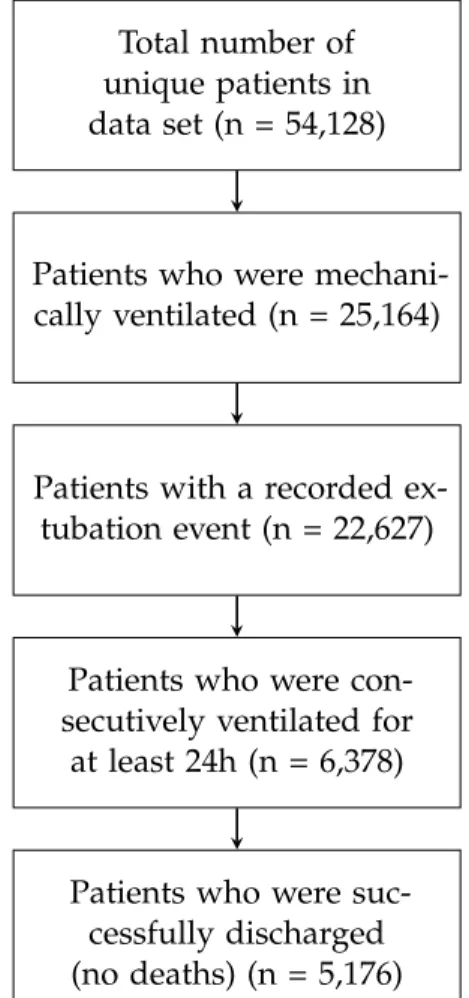
Analogously to previous reinforcement learning research in the field of weaning mechanically ventilated patients [7, 8, 9], we only consider patient histories meeting the following criteria:

• The patient was mechanically ventilated for at least 24 consecutive hours. This is to exclude short routine ventilations after surgery with low risk of complications.

• An extubation event, successful or not, is recorded in the data. The outcome of this event can then be used as a reward for a learning agent.

• The patient was successfully discharged from the ICU, i.e. did not die. Death usually occurs due to a wide variety of reasons beyond the scope of weaning.

(19)

3. Methods

Out of the 54,128 unique patients in theHIRID2data set, 5,176 are included in this study, see Figure 3.1. This is around twice as many as the 2,464 patients included in previous reinforcement learning research on weaning [7, 8, 9]. However, it is less than the 20,940 patients included in the sepsis study using NOSVP as reinforcement learning algorithm [6].

Total number of unique patients in data set (n = 54,128)

Patients who were mechanically ventilated (n = 25,164)

Patients with a recorded extubation event (n = 22,627)

Patients who were con- secutively ventilated for at least 24h (n = 6,378)

Patients who were successfully discharged (no deaths) (n = 5,176)

Figure 3.1: Patient inclusion statistics

3.2 MDP definition

As introduced in section 2.2, we use the MDP framework to define our reinforcement learning structure. The environment, corresponding to the state spaceS, is the patient and the current therapeutic settings, such as the ventilator mode or amount of oxygen delivered. At every time stept, the agent is in a state st ∈ S and, in case the state is non-terminal, takes an action a_t ∈ A, yielding a next states_t+1 ∈ S and a rewardr_t+1 ∈ R with probabil-

(20)

3.2. MDP definition ity p(s_t+1,r_t+1|s_t,a_t). In the following we define the spaces S,A, Ras well

as the transition function p.

State space S

We use a set of 22 patient and therapy related variables whose values we then map to a total of 200 different states, see subsection 3.3.1 and subsection 3.3.4 for more details. Therefore, our state space looks as follows:

S ={s₀,s₁, . . . ,s₁₉₉}

Table 3.1 lists all 22 variables used in this study. Thevm value in parenthe- ses corresponds to the variable name in theHIRID2 time series. An asterisk indicates newly engineered variables not present in the original data set, either created by the previous research team working with the data (∗₁) or created specifically for this thesis (∗₂), see subsection 3.3.1.

Age

Arterial oxygen saturation (S_aO₂; vm141) Arterial partial pressure of oxygen (P_aO₂)∗₁ Arterial pH (vm138)

Body mass index (BMI)∗₂ Body temperature (vm2) Extubation readiness∗₁

Fraction of inspired oxygen (FiO₂; vm58) Gender

Heart rate (vm1)

Peripheral oxygen saturation (SpO₂; vm20) Positive end-expiratory pressure (PEEP; vm59) Previously ventilated during same ICU stay∗₂ Reason for ventilation (vm229)

Respiratory rate (vm22)

Richmond Agitation-Sedation Scale (RASS; vm28) Spontaneous breathing (vm224)

Supplemental fraction of inspired oxygen (FiO₂; vm309) Supplemental oxygen (vm23)

Systolic blood pressure (vm3) Time on the ventilator∗₂ Ventilator mode group (vm306)

Table 3.1: Clinical variables used

(21)

3. Methods

Action space A

Analogously to previous work [7, 8, 9], we consider actions along two dimen- sions: sedation levels and having the patient either on or off the ventilator.

After consultation with an intensive care physician, we decide against using dosages of sedatives directly, since their sedation effect can depend on a variety of factors, including how long a drug has already been administered for. Instead, the negative portion of the Richmond Agitation–Sedation Scale (RASS) is used to approximate the patient’s sedation level. The RASS score ranges over 10 discrete values from -5 to 4 and is used in critical care to clinically asses a patient’s sedation and agitation level [20]:

• A negative value indicates a sedated patient, -5 being the highest sedation level corresponding to an unarousable patient

• A positive value indicates a fully awake and agitated patient, the highest value of 4 corresponding to combative behavior

• A value of zero indicates a fully awake and calm patient

We use the RASS score as follows to approximate a patients sedation level ranging from 0 to 5: |min(RASS, 0)|. Additionally, on a second dimension, we indicate whether we leave the patient on the ventilator (0) or extubate them (1). This yields the following two-dimensional action space with a total of twelve possible actions:

A= 0

0

, 0

1

, 0

2

, 0

3

, 0

4

, 0

5

, 1

0

, 1

1

, 1

2

, 1

3

, 1

4

, 1

5

Reward R

We pursue two goals simultaneously, a successful extubation (clinically sta- ble, no reintubation in the future) while minimizing the time spent on the ventilator. We therefore define a small negative reward for each ventilation hour of -0.5, a large positive reward of 100 for a successful extubation and a large negative reward of -100 for an unsuccessful extubation. The reward space thus looks as follows:

R={−100,−0.5, 100}

In order to assign a positive or negative reward depending on the outcome of the extubation attempt, a corresponding variable in the data set is used. The variable was engineered by the research team who preprocessed the critical care data set prior to this thesis. It indicates that an extubation event is not successful in case that the patient needs to be reintubated during the same ICU stay or in case that the patient is clinically unstable after extubation but does not require reintubation. In all other cases extubation is considered successful.

(22)

3.3. Preprocessing Since the mathematical convergence guarantees for the NOSVP algorithm

only hold for non-negative rewards, see section 2.3, we use the same approach to the reward function as in [6], i.e. limiting negative rewards to the last point in time for each trajectory and falling back to the greedy action selection in caseV(s)is negative for a states. However, in order to still have the incentive for the agent to keep ventilation periods as short as possible, we use the reward ofr = −0.5 per ventilation hour in our average reward scoring function (see subsection 3.5.1) which is then used to find the optimal parameterγon the validation set during training. Sinceγis a trade-off parameter between short-term and long-term rewards, we therefore use an implicit negative reward per time step during training and an explicit one during validation and testing. In order to make the different policies com- parable, we apply this approach to all of our learning algorithms, not just to NOSVP.

Transition function p

Two of the reinforcement learning algorithms used in this thesis, Q-learning and NOSVP, are model-free algorithms, meaning they assume no knowledge about the inner workings of the environment and therefore of the transition function. Value iteration, on the other hand, is model-based and requires a transition function, which we approximate as follows: For each state-action pair(s,a)observed in the clinical data set, we estimate the probability of the next state beings⁰ by summing up all corresponding instances and dividing the sum by the total sum of all next states. Additionally to the value iteration algorithm, we use this approximated transition function in the average reward scoring function to simulate policies on the test and validation set, see subsection 3.5.1.

3.3 Preprocessing

As mentioned before, some preprocessing steps, including imputing miss- ing values and engineering of new variables, e.g. whether an extubation was successful or not, were already performed prior to this thesis. How- ever, in order to get the data into a form required for training, additional preprocessing steps are required, which are explained in this section.

3.3.1 Trajectory selection and additional variables

Since some patients in the data set were mechanically ventilated for more than one episode during their stay at the ICU, we treat each episode as a distinct patient trajectory in order to best use all data points available. For each ventilation trajectory we then then check whether all inclusion criteria

(23)

3. Methods

(see Figure 3.1) are met, especially whether the trajectory is at least 24h long.

If not, the trajectory is discarded. Next, we create four additional variables:

1. A Boolean variable indicating if a trajectory is the first ventilation episode or if a patient has been ventilated before

2. A variable of how long the patient has already been ventilated for during the current trajectory

3. The body mass index, calculated as _m^kg2 from the weight and height of the patient as recorded in the data set

4. An approximation to the patients health status (see subsection 3.5.2).

This variable is not used for training. Instead, in chapter 4, it allows us to assign a certain clinical meaning to the various states in our state spaceS.

3.3.2 Downsampling

Fundamentally, the sampling rate or temporal resolution is a trade-off between training speed (low temporal resolution) and a potentially higher accuracy (high temporal resolution). In order to learn about the effect of the temporal resolution, we downsample the data to three different time steps in this thesis, 15min, 1h and 4h intervals and compare the results in chapter 4. The last, 4h time steps, is analogous to previous NOSVP research in the clinical setting [6]. Whenever we perform an analysis on only one of the three different sampling rates, we indicate which one we use. However, in chapter 4, the most important metrics are presented for all three sampling rates.

3.3.3 Data split

We split the data into three distinct sets as follows:

• Training set (70%)

• Test set (20%)

• Validation set (10%)

In order to avoid adding correlations to the data, we ensure that trajectories stemming from the same patient always end up in the same data set.

3.3.4 Scaling and clustering

We cluster our data into a discrete set of states using k-means, again anolo- gously to the previous medical NOSVP implementation [6, 10]. In order to avoid biases towards variables with very large ranges, we first scale the entire data set, thereby trying three different scaling methods provided by the

(24)

3.3. Preprocessing scikit-learn framework, MinMaxScaler, RobustScaler and RobustScaler with

a prior PowerTransform [21]. Since for our metrics MinMaxScaler performs best (see section A.1 in the Appendix), we use the MinMaxScaler before clustering our data. It scales all variables into the range [0,1] while leaving the underlying distribution unchanged. The scaler is first fitted with the training set and then applied to all three data sets.

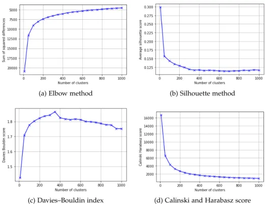
Next, we aim to find the optimal number of clusters. Here we use a total of four different metrics, the elbow method, the silhouette method [22], the Davies–Bouldin index [23] and the Calinski and Harabasz score [24]. How- ever, the different methods yield rather different optimal numbers of clusters. While the Silhouette and Calinski and Harabasz methods score highest for very low number of states, here 10, the Elbow method suggests around 100 states and the Davies–Bouldin index around 350 states, see Figure 3.2 for an overview. Since, in the end, we try to find the number of clusters yielding the best performance for our NOSVP algorithm, we then decide to run our preprocessing and training pipeline for a range of different cluster numbers, compare the results (see section A.2 in the Appendix) and finally choose to use 200 states.

(a) Elbow method (b) Silhouette method

(c) Davies–Bouldin index (d) Calinski and Harabasz score

Figure 3.2: Comparison of different clustering metrics. For each, a point higher up on the curve corresponds to a better performance.

(25)

3. Methods

In order to create the 200 states for our state spaceS, we first fit the k-means clustering algorithm to the training set, then predict the clusters for all three data sets.

3.3.5 SARSA trajectories

In this last preprocessing step, we bring each ventilationtrajectory_i of length t_iinto the following form, withdonebeing a Boolean variable indicating the end of the trajectory, i.e.done_t_i =True:

trajectory_i =s₀,a₀,r₁,s₁,a₁,done₁, . . . ,s_t_i₋₁,a_t_i₋₁,r_t_i,None,None,done_t_i This is analogous to SARSA, the name indicating (s,a,r⁰,s⁰,a⁰)episodes as input, another reinforcement learning algorithm which we do not evaluate in this thesis. However, the generality of this data structure allows it to be used for a wide range of reinforcement learning algorithms.

3.4 Learning

With the training set of SARSA trajectories as input, we use a total of six different approaches to find a policyπfor weaning mechanically ventilated patients. For reinforcement algorithms using γ as a trade-off parameter between short-term and long-term rewards, we use our validation set in order to find the value forγwith the best performance.

Four out of the six policies are deterministic, i.e. for each state they return exactly one action deemed optimal: π_{naive max}, πnaive random, π_QL and π_{V I}. On the other hand,π_empiricalis probabilistic, returning a probability for each action given a state as input. In a sense, π_NOSVP can also be seen as a probabilistic policy. However, in this case with a uniform distribution and only over the actions returned for a state given as input, not over the entire action spaceA_.

Analogously to Tang et al. [6], we want to exclude actions which seem highly unlikely with the given data set. Therefore, we create anaction mask that excludes all actions which were seen less than five times for a given state in the training set. If for a state no action is seen at least five times, the most common action is kept, thereby ensuring that every state has at least one action. The action mask is applied to all our learning algorithms.

In this section, we explain our methods for finding different policies using the training and validation sets, chapter 4 is then dedicated to the evaluation and performance comparison using the test set of our data.

(26)

3.4. Learning 3.4.1 Empirical policy

Given the training set, for each of the 200 states we determine the probability of each action. Thus, for some states ∈ S, theempirical policy π_empiricallooks as follows, whereby all actions masked out by our action mask have their probability set to 0:

π_empirical(s) ={a₀: p_s,a₀, a₁: p_s,a₁, . . . , a₁₁: p_s,a₁₁}

Sinceπ_empirical is built with the actual actions taken by clinicians as recorded in the critical care data set, it is an approximation of how clinicians decide based on current clinical guidelines for managing mechanically ventilated patients in the ICU. This provides an interesting basis for comparison with our other learning algorithms.

3.4.2 Naive policy

In order to have additional performance baselines and sanity checks, we build two naive policies, π_{naive max} and πnaive random, based on the simple as- sumption that either the most common or a random action could perform best for each state.

Most common action

The first of our naive policies always chooses the most common action for every state as seen in the training set. Therefore, π_{naive max} looks as follows in terms of π_empirical for some states ∈ S:

π_{naive max}(s) =max

a∈A

π_empirical(s)(a)

Random action

The second naive policy chooses a random action for every state. Thus, πnaive random looks as follows in terms ofπ_empirical for some states∈ S:

πnaive random(s) =random choice{a∈π_empirical(s)}

3.4.3 Q-learning

Q-learning is a classical reinforcement learning algorithm first introduced in 1989 [25]. It is the conceptual basis for many of the powerful contem- porary reinforcement learning approaches, especially deep Q-learning [26]

introduced in 2013 and its derivations. Also, for the NOSVP algorithm as implemented in [6] and adapted for our objective, Q-learning plays a funda- mental role: Its value function V_QL is used by NOSVP as an input, thereby assumed to be an approximation of V^∗, the optimal value function. Besides

(27)

3. Methods

being a prerequisite for NOSVP, we also use Q-learning as a standalone algorithm in this thesis and evaluate and compare its performance to the other algorithms in chapter 4.

Q-learning is model-free, i.e. does not require the transition function p.

Instead it uses a technique called temporal difference learning to bootstrap from the current estimation of the value function [5]. Since our state-action- space is small enough to fit into memory, we directly store all Q values, an approach calledtabular Q-learning [5]. See algorithm 1 for the pseudocode of our implementation of tabular Q-learning.

For α we use an exponential decay over the number of episodes with a starting value ofα_t=0=0.9 as follows:

α_t =10⁻¹⁰+ (0.9−10⁻¹⁰)e⁻¹⁰⁻²^b^t/1000^c

In order to find the optimal value for γ, Q-learning is run in parallel for a range of different candidate values and then scored on the validation set with our average reward scoring function (see subsection 3.5.1).

Algorithm 1:Tabular Q-learning Input: trajectories,αt,γ∈ (0, 1] initialize: Q(s,a) =0∀s∈ S,∀a∈ A forall episodesdo

choose randomtrajectoryfrom trajectories foreach step in trajectorydo

observes,a,r,s⁰ from trajectorystep Q(s,a)← Q(s,a) +αt[r+γmax

a⁰∈AQ(s⁰,a⁰)−Q(s,a)]

end end

3.4.4 Value iteration

In contrast to Q-learning and NOSVP,value iteration does not use the ventilation trajectories as input directly but instead relies on our approximated transition functionp, i.e. value iteration is model-based. See algorithm 2 for the pseudocode of our implementation of value iteration.

The termination variableθis set toθ=10⁻¹⁰. Analogously to our Q-learning implementation, we find the optimalγ by running a range of different values in parallel and testing them on the validation set.

(28)

3.5. Evaluation Algorithm 2:Value iteration

Input: transition function p,γ∈(_{0, 1}]_,θ >₀ initialize: V(s) =0∀s∈ S,δ=0

whileδ ≥θ do forall s∈ S _do

v←V(s) V(s)←max

a∈A ∑

s⁰,r

p(s⁰,r|s,a)(r+γV(s⁰)) δ←max(δ,|v−V(s)|)

end end

3.4.5 Near-optimal set-valued policy

Near-optimal set-valued policy(NOSVP), as introduced in 2011 [17] and further refined in 2020 [6], is a novel approach to reinforcement learning, especially suited for systems recommending actions to humans, in our case critical care clinicians. Its novelty lies in the fact that the algorithm does not attempt to find a policy with the optimal action for each state but rather a set of actions yielding a near-optimal outcome.

The NOSVP algorithm is very similar to Q-learning in its implementation.

The main difference being that NOSVP uses a variable ζ to include all actions that lead to an expected reward of at least (1−ζ)V^∗(s). Thereby, the optimal value function V^∗ is approximated by V_QL. In case the algorithm is not successful in identifying a set of near-equivalent actions, it falls back to the greedy action selection, i.e. Q-learning. See the corresponding code annotations in algorithm 3, the pseudocode of our NOSVP implementation.

We use the same exponentially decayingα_tas for Q-learning. The algorithm is run for a range of five different zetas, ζ ∈ {0.0, 0.05, 0.1, 0.15, 0.2}. For each, we again find the optimalγby running the algorithm in parallel for a range of different values and scoring them on the validation set. Note that NOSVP for ζ =0 equals Q-learning.

3.5 Evaluation

In order to evaluate the different policies and better understand the data, we create several evaluation metrics described in this section. The actual performance analysis then follows in chapter 4.

(29)

3. Methods

Algorithm 3:Near-optimal set-valued policy Input: trajectories,V^∗,αt,γ∈(0, 1]ζ ∈[0, 1) initialize: Q(s,a) =0∀s∈ S,∀a∈ A

forall episodesdo

choose randomtrajectoryfrom trajectories foreach step in trajectorydo

observes,a,r,s⁰ from trajectorystep π(s⁰) ={a⁰ |Q(s⁰,a⁰)≥(1−ζ)V^∗(s⁰)}

ifπ(s⁰)6=_∅then // select the worst best action Q(s,a)←Q(s,a) +α_t[r+γ min

a⁰∈π(s⁰)Q(s⁰,a⁰)−Q(s,a)]

else // fall back to the greedy action Q(s,a)←Q(s,a) +α_t[r+γmax

a⁰∈AQ(s⁰,a⁰)−Q(s,a)]

end end end

3.5.1 Average reward scoring

The performance of a policy is measured as the average reward it scores on clinical data. This is done in a probabilistic fashion:

1. For a given data set (test set or validation set), the transition function p(s⁰,r|s,a)is estimated

2. All starting states for the trajectories seen in the the data set are stored 3. 100,000 test runs are performed and the rewards averaged and re-

turned as score. Each test run starts in a state randomly selected from the previously stored starting states with the same underlying distribution as in the data set. Then, for every action taken, the next state is chosen randomly according to the probability p(s⁰,r|s,a). For policies with more than one action per state, the action is either chosen uniformly at random (NOSVP, since we assume every action in the near-optimality set is equal) or random with the underlying probabilities (empirical policy).

Because the average reward scoring function takes as input a data set (test set or validation set) and then estimates the transition function p based on that data set, p only contains transition probabilities that were seen in that particular data set. However, our algorithms are trained on a different data set, the training set. It is therefore possible that a policy contains state- action pairs which are never encountered in the data set used as input for the average reward scoring function. Should the policy choose an action for a state for which we have no information with the given data set, then the

(30)

3.5. Evaluation current test run gets aborted and no rewards are stored for that run. The

average reward scoring function records the percentage of successful runs and returns it, allowing us to analyze the completion rate of a policy on a given data set.

In order to guarantee termination of the average reward scoring function even for policies which never extubate a patient, a reward is either stored when the patient gets extubated or when the cumulative reward is equal to or below -100. Consequently, each run yields a reward in the range from -199.5 to 100. The lowest case, -199.5, happens when an agent has accumu- lated -99.5 in negative step rewards, just below the threshold of -100, and then tries to unsuccessfully extubate the patient, receiving an additional reward of -100 for a total of -199.5. The highest possible score of 100 is possible if the agent successfully extubates a patient in the first time step, without having received any negative step rewards.

The average reward scoring is used for two purposes in our machine learning model—for finding the optimalγwith the validation set during training and for comparing the performance of the different policies on the test set in chapter 4. The implementation of the average reward scoring function is parallelized, allowing for increased performance in a multiprocessor environment such as ethsec / Leonhard.

3.5.2 Clinical score

In order to better understand the meaning behind the different states, a subset of the Simplified Acute Physiology Score (SAPS) II[27] is used, taking into account the following variables: age, heart rate, systolic blood pressure, temperature and the PaO₂/FiO₂ratio. Note that in the original score, PaO₂/FiO₂ is considered to yield zero points irrespective of the actual values if the patient is not mechanically ventilated. Since in our trajectories this is never the case, our adapted score starts at 6 instead of 0. At the other end of the spectrum, the highest possible score is 56 for our adaptation. See Table 3.2 for an overview of how the score is calculated based on the original score [28].

3.5.3 Distance to the empirical policy

The empirical policy, as estimated from the training set, can be seen as a form of ground truth for the clinical data. It is therefore interesting to have a distance measure of how far a policy is to the empirical policy. Two different scores are used to measure this distance:

• The average percentage per state that the empirical policy would have chosen the same action(s). Since the empirical policy is a probabilistic policy, the highest possible score for this metric will be achieved by the

(31)

3. Methods

Characteristic Values Score

Age (years)

<40 0

40−59 7

60−₆₉ ₁₂ 70−74 15 75−79 16

≥80 18

Heart rate

<40 11

40−69 2

70−119 0

120−159 4

≥160 7

Systolic blood pressure

<70 13

70−99 5

100−199 0

≥200 2

Temperature <39 0

≥39 3

P_aO₂/FiO₂

<100 11

100−199 9

≥200 6

Table 3.2: Subset of SAPS II used as clinical score, yielding a value in the range [6, 56].

naive policy choosing always the most common action as seen in the training data.

• The average sum of squared differences per state for the 3 most common actions of the empirical policy. Is the action of the policy under evaluation among the three most likely actions of the empirical policy, then that sum is zero. Otherwise the distance along the sedation and the ventilation axes are measured separately on a scale from 0 to 1.

For the NOSVP policy with more than one action per state the closest action to the empirical policy is used.

(32)

3.5. Evaluation 3.5.4 NOSVP intra-policy distance

While the measure described in subsection 3.5.3 is an inter-policy score, for the NOSVP policy it is also interesting to see how closely together the rec- ommended actions are, i.e. an intra-policy score. The results then give an intuitive sense of how realistic an NOSVP policy is: Are the actions recom- mended for a certain state far apart on the sedation and/or ventilation axis, then those actions seem less likely to provide meaningful recommendations.

On the other hand, having the patient e.g. on ventilation level 3 instead of 2 or 4 is more likely to be an actual choice in clinical practice.

(33)

(34)

Chapter 4 Results

In this chapter, we evaluate and compare our different policies. First we look at the convergence behavior and measured runtimes in section 4.1, then in section 4.2 at the general performance of the different approaches, and finally in section 4.3 we turn our attention to the properties of our NOSVP algorithm. Recall that we use three different sampling rates of the critical care data set, 15min, 1h and 4h intervals. While generally we present the results for a temporal resolution of 1h time steps, the most important metrics are presented for all three sampling rates, allowing for a direct comparison the temporal resolution has on our algorithms.

4.1 Convergence and time complexity

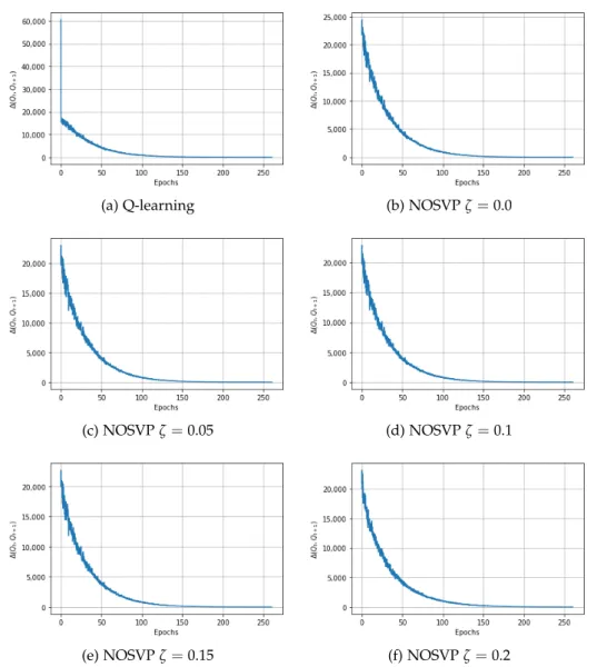
In order to evaluate the convergence behavior of Q-learning and NOSVP, we take a similar approach to the authors of the 2017 reinforcement learning weaning paper [7]. We compare consecutive Q tables stored during training, measure their Euclidean distance and plot the result for the number of epochs the algorithm runs for. However, it is worth pointing out that since our learning algorithms choose patient trajectories in a random fashion, epochin our context merely refers to a number of selected trajectories equal to the size of the training set, not that the training set has been consumed in its entirety. Figure 4.1 shows the corresponding convergence curves for a 1h sampling rate. As can be seen, all algorithms manage to converge after around 150 epochs.

For the runtime comparison of our learning algorithms we use the training set with 3,837 unique ventilation trajectories and a state space of 200 different states. Furthermore, we use all three of our different data sampling rates, 15min, 1h and 4h intervals. All times are measured without any par- allelization and on a single processor. For the value iteration algorithm the time indicated includes the time spent on first building the required approx-

(35)

4. Results

(a) Q-learning (b) NOSVPζ=0.0

(c) NOSVPζ=0.05 (d) NOSVPζ=0.1

(e) NOSVPζ=0.15 (f) NOSVPζ=0.2

Figure 4.1: Convergence behavior for Q-learning and NOSVP on the training set with a 1h sampling rate. The y-axis corresponds to the Euclidean distance between consecutive Q-tables during training.

imated transition function p. Note that NOSVP needs as one of its inputs V^∗, approximated byV_QL. It is therefore necessary to run Q-learning before- hand. Nevertheless, the indicated execution times for NOSVP in Table 4.1 only refer to the NOSVP part and do not include running Q-learning.

(36)

4.2. Policy performance comparison

Algorithm 15min 1h 4h

Value iteration 00:00:03 00:00:02 00:00:02 Q-learning 02:25:13 00:42:43 00:14:11 NOSVPζ =_0.1 _04:52:35 _01:12:33 _00:16:50

Table 4.1: Runtimes on the training set with different sampling rates

4.2 Policy performance comparison

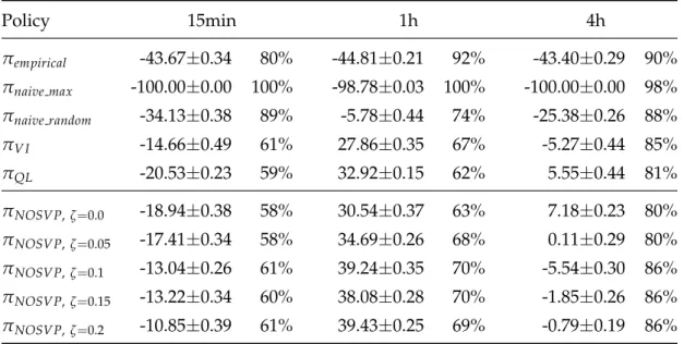
Using our average reward scoring function, we can compare the performance of the different policies on the test set of our data. Table 4.2 gives an overview of the average scores including standard deviations for each algorithm and sampling rate. Recall that our average reward scoring function (see subsection 3.5.1) uses the test or validation set as input which might not contain state-action pairs that an algorithm learned on the training set. A test run can therefore only be completed if the action chosen for a state by a policy also shows up in at least one patient trajectory in the input data, here the test set. The percentage of complete test runs is also indicated in Table 4.2.

Policy 15min 1h 4h

π_empirical -43.67±0.34 80% -44.81±0.21 92% -43.40±0.29 90%

π_{naive max} -100.00±0.00 100% -98.78±0.03 100% -100.00±0.00 98%

πnaive random -34.13±0.38 89% -5.78±0.44 74% -25.38±0.26 88%

π_{V I} -14.66±_0.49 _61% _27.86±_0.35 _67% _-5.27±_0.44 _85%

π_QL -20.53±0.23 59% 32.92±0.15 62% 5.55±0.44 81%

π_NOSVP,_ζ₌_0.0 -18.94±0.38 58% 30.54±0.37 63% 7.18±0.23 80%

π_NOSVP,_ζ=0.05 -17.41±0.34 58% 34.69±0.26 68% 0.11±0.29 80%

π_NOSVP,_ζ=0.1 -13.04±0.26 61% 39.24±0.35 70% -5.54±0.30 86%

π_NOSVP,_ζ=0.15 -13.22±0.34 60% 38.08±0.28 70% -1.85±0.26 86%

π_NOSVP,_ζ=0.2 -10.85±0.39 61% 39.43±0.25 69% -0.79±0.19 86%

Table 4.2: Average rewards scored by our policies on the test set with different sampling rates, including standard deviations. The percentage to the right indicates how often the choices made by the policy were feasible on the test set, i.e. the completion rate of test runs.

(37)

4. Results

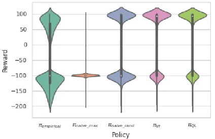
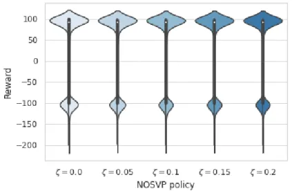
In order to better understand the distribution of rewards received, we use the results of the 100,000 test runs during average reward scoring for the creation of violin plots. See Figure 4.2 for plots for the baseline algorithms π_empirical, π_{naive max}, πnaive random, π_{V I} and π_QL. Figure 4.3 then depicts the violin plots for our NOSVP algorithm for the different ζ values. All plots were created based on a data sampling rate of 1h.

Figure 4.2: Violin plots for the rewards received by the baseline algorithms on the test set with a 1h sampling rate. The box plot inside the kernel density estimation indicates the median (white dot), first quartile and third quartile (end points of thick line) as well as the lower and upper adjacent values (end points of thin line).

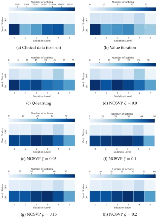
The 12 actions in our action spaceAcarry a direct clinical meaning pertain- ing to the management of mechanically ventilated patients. It is therefore interesting to see how frequent each action is in the clinical data set as well as how often our policies choose each action. Figure 4.4 gives an overview of these action frequencies. Note that since we try to keep ventilation periods short, extubation actions (the top six actions in the plots in Figure 4.4) show up with a higher frequency in the policies of our learning algorithms compared to the clinical data, here the test set.

4.3 Near-optimal set-valued policies

In this section, we evaluate the NOSVP algorithm and its behavior for our weaning objective and critical care data set more closely.

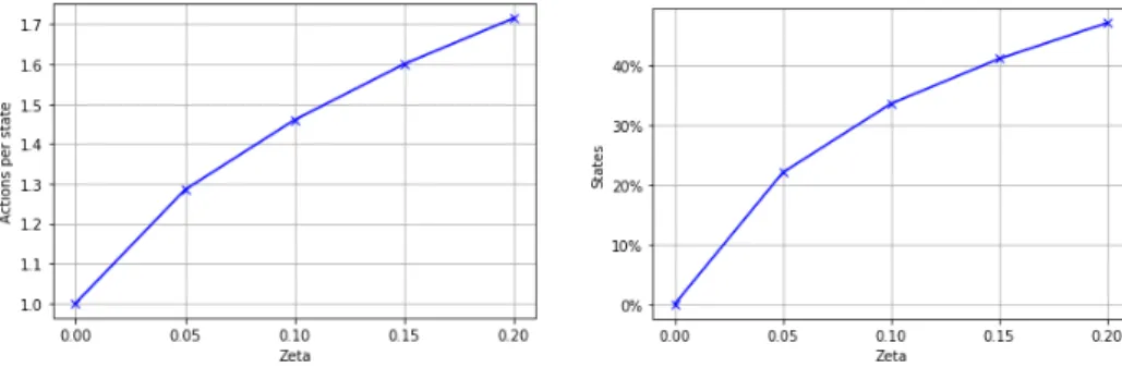
Sinceζ is a trade-off parameter between policy performance and policy size (the number of actions proposed for each state), the number of actions per

(38)

4.3. Near-optimal set-valued policies

Figure 4.3: Violin plots for the rewards received by NOSVP on the test set with a 1h sampling rate. The box plot inside the kernel density estimation indicates the median (white dot), first quartile and third quartile (end points of thick line) as well as the lower and upper adjacent value (end points of thin line).

state as well as the percentage of states with more than one action increase with higherζ values, as is shown in Figure 4.5.

NOSVP uses as one of its inputs a value function it considers optimal, V^∗, approximated byV_QL. Next, instead of choosing the greedy action based on V^∗, NOSVP chooses a set of near-greedy and therefore near-optimal actions, with the near-optimality defined byζ. Consequently, it is interesting to see which additional actions NOSVP selects for each greedy or optimal action.

This is shown with the heat maps in Figure 4.6 for our different values of ζ. The greedy action is marked in a blue square, other actions are colored according to the frequency they are chosen additionally to the greedy action. The small number in blue at the bottom right indicates how often the corresponding action is in fact considered optimal. Note that for ζ = 0.0 no additional actions are chosen by NOSVP, i.e. this corresponds to solely greedy action selection.

Using our clinical score as introduced in subsection 3.5.2, we can evaluate how NOSVP behaves depending on a patient’s current health status.

First, we score each point in time for each patient in the original data set.

Then, after clustering, we average the scores of patient time points which are mapped into the same of our 200 states. In the end we segment the states into three different groups according to their average clinical score, [0,10], (10,25] and (25,56]. Note that a higher clinical score corresponds to

(39)

4. Results

(a) Clinical data (test set) (b) Value iteration

(c) Q-learning (d) NOSVPζ=0.0

(e) NOSVPζ=0.05 (f) NOSVPζ=0.1

(g) NOSVPζ=0.15 (h) NOSVPζ=0.2

Figure 4.4: Comparison of action frequencies in the critical care data set and for the different policies trained on the training set with a 1h sampling rate.

(40)

(a) Average number of actions per state (b) States with more than one action

Figure 4.5: NOSVP policy behavior for increasing values of ζ after training on the training set with a 1h sampling rate.

a sicker patient. In Figure 4.7 we compare these score groups to the policy size, i.e. the average number of actions our NOSVP algorithm with ζ =0.1 proposes per state. Figure 4.8 then shows the value function V_NOSVPζ=0.1

for the different score groups, indicating the expected reward for each of the three groups.

Finally, to get a deeper understanding of how NOSVP could behave in practice, we look at a sample patient trajectory from the test set with a 1h sampling rate. The 51 year old patient was being mechanically ventilated for a total of 50 hours, we thereby zoom in on the section from 10 to 12 hours as depicted in Figure 4.9. For each of the three hours we list the most important variables whose values change over the course of the observed time frame. The actions are given as two-dimensional vectors as introduced in section 3.2, indicating both the ventilation status as well as the sedation level. Note that the RASS score is not listed since it is already implied in the actions taken. NOSVP with ζ = 0.1 proposes two different actions for the time point t_vent = 11h, ₀

0

and ₁

0

, drawn in blue. The former action was also the one taken by the clinicians treating the patient, leading to the patient status in tvent = 12h. The latter action would have extubated the patient while leaving the sedation level at zero. Also note the state the three time points are mapped to in our state space S as indicated at the bottom.

Incidentally, the variable values at tvent = _{10h and} _t_vent = 12h map to the same state 76. After 50 hours of mechanical ventilation the patient was unsuccessfully extubated (not shown), also with variable values mapping to state 44 as for t_vent =_11h.

(41)

4. Results

(a) NOSVPζ=0.0

(b) NOSVPζ=0.05

(c) NOSVPζ=0.1

(d) NOSVPζ=0.15

(e) NOSVPζ=0.2

Figure 4.6: Action heat map for different values ofζindicating the frequency of actions proposed by NOSVP in addition to the greedy action (blue square) after training on the training set with a 1h sampling rate. The small number in blue at the bottom right indicates how often the corresponding greedy action is considered optimal.

(42)

Figure 4.7: Violin plots showing the number of actions per state for different clinical score ranges for NOSVP ζ = 0.1 on the test set with a 1h sampling rate. A higher clinical score corresponds to sicker patients. The violin plots are cut so that only values corresponding to actual data points are shown. The box plot inside the kernel density estimation indicates the median (white dot), first quartile and third quartile (end points of thick line) as well as the lower and upper adjacent value (end points of thin line).

(43)

4. Results

Figure 4.8: Violin plots showing the value function V_NOSVP_ζ=0.1 for states on the test set with a 1h sampling rate and different clinical score ranges. A higher clinical score corresponds to sicker patients. The violin plots are cut so that only values corresponding to actual data points are shown. The box plot inside the kernel density estimation indicates the median (white dot), first quartile and third quartile (end points of thick line) as well as the lower and upper adjacent value (end points of thin line).

t_vent 10:00 aPH 7.37 aSO2 94.90 Ext.r. no FiO₂ 0.50 PaO2 81.63 PEEP 4.90 RR 25.90 State 76

t_vent 11:00 aPH 7.43 aSO2 97.50 Ext.r. yes FiO₂ 0.50 PaO2 83.96 PEEP 5.20 RR 17.50 State 44

t_vent 12:00 aPH 7.43 aSO2 97.50 Ext.r. no FiO₂ 0.49 PaO2 68.98 PEEP 4.80 RR 23.30 State 76

Extubation ₀

2

₀

0

₁

0

₀

3

₀

2

Figure 4.9: Part of a sample trajectory in the critical care data set of a 51 year old patient being mechanically ventilated. The two actions proposed by NOSVP with ζ = 0.1 at t_vent = 11h are drawn in blue. The state at the bottom indicates to which state the patient variables are mapped to in our state spaceS. Ext.r.: extubation readiness; RR: respiratory rate.